Thermodynamics of $O(3)$ Classical Heisenberg Model in Multipath Metropolis Simulation

Abstract

We study the thermodynamics of classical Heisenberg model using the multipath approach to Metropolis algorithm Monte Carlo simulation. This simulation approach produces uncorrelated results with known precision. Also, it can be easily generalized to other classical models of magnetism. Comparing results obtained from multipath and from single–path simulations we demonstrate that these approaches produce equivalent results.

1 Introduction

Classical lattice models attract attention nowadays for several reasons. Classical Heisenberg model is frequently used in Monte Carlo simulations of nonlinear sigma models [1], and also for modeling real compounds [2, 3, 4] and other systems [5, 6]. In the recent paper [7] multipath Metropolis simulation of $O(3)$ classical Heisenberg model is introduced. Since multipath approach is embarrassingly parallelizable, it utilizes easily computing power of any number of computing elements and provides normally distributed results with desired precision. One of the main advantages of the multipath Metropolis simulation is its applicability to many different classical lattice models, such as Ising [8, 9, 10], Potts [11, 12] etc. The multipath approach allows complete control over the simulation in a sense that it is possible to conduct a ”short simulation” in order to make a reasonable estimate. Later, the simulation precision can be incrementally improved with additional, subsequently computed results. This is of great practical importance as it turns out that the optimal simulation parameters (number of lattice sweeps and the number of simulation paths), strongly depend on the temperature and lattice size.

The simulation results presented in this paper were computed using free software C++ library called ”Hypermo” [13] on computing services of the Supercomputing Center of Galicia (CESGA) [14]. The figures are created using ”Tulipko” [15] interactive visualization tool.

2 Model and simulation

The Hamiltonian of classical $O(3)$ Heisenberg model is

$$H=-\frac{J}{2}\sum_{\bm{n},\bm{\lambda}}\bm{S}_{\bm{n}}\cdot\bm{S}_{\bm{n}+\bm{\lambda}},$$ (1)

where the summation is taken over all lattice sites $\{\bm{n}\}$ with total $N=L^{3}$ sites of simple cubic lattice, and $\bm{\lambda}$ connects a given site to its nearest neighbors. The convinient energy scale is set by $J=k_{\mathsf{B}}=1$ and we use the standard spherical parametrization for spin vectors

$$\bm{S}_{\bm{n}}=[\sin\theta_{\bm{n}}\cos\varphi_{\bm{n}},\sin\theta_{\bm{n}}\sin\varphi_{\bm{n}},\cos\theta_{\bm{n}}]^{\mathsf{T}}.$$ (2)

The quantities of interest are the total spin

$$\bm{M}=\frac{1}{N}\sum_{\bm{n}}\bm{S_{\bm{n}}},$$ (3)

of which the average value is magnetization $\langle\bm{M}\rangle$ , the internal energy of the system $\langle H\rangle$, magnetic susceptibility

$$\chi(T)=\frac{L^{3}}{T}\left[\langle|\bm{M}|^{2}\rangle-\langle|\bm{M}|\rangle^{2}\right],$$ (4)

and capacity

$$C_{V}(T)=\frac{L^{3}}{T^{2}}\left[\langle H^{2}\rangle-\langle H\rangle^{2}\right].$$ (5)

Because there can’t be no spontaneous symmetry breaking in finite lattices magnetic susceptibility is defined with

$$|\bm{M}|=\frac{1}{N}\Big{|}\sum_{\bm{n}}\bm{S_{\bm{n}}}\Big{|}.$$ (6)

In multipath approach, each simulation consists of a certain number $\mathcal{N}$ of simulation paths (simulation path, SP). Each SP produces output. Outputs of all the $\mathcal{N}$ SPs, together, form a simulation output (SO). Monte Carlo averages are then computed as

$$\langle A\rangle=\frac{1}{\mathcal{N}}\sum_{i=1}^{\mathcal{N}}A_{i}$$ (7)

and $\chi$ and $C_{V}$ are calculated from (4) and (5). It should be noted that all thermodynamic quantities in the paper are calculated per lattice site.

Multipath Metropolis simulation can be easily visualized in the phase space of the lattice, which is the direct product of the two-spheres $\mathcal{S}^{\mathbf{2}}$ located at lattice sites.

Figure 1: (Color online) Illustration of the lattice phase space trajectories in the multipath simulation at low temperature for random initial state. Each line represents one path.

Figure 1 illustrates multipath simulation in the lattice phase space ($PS$) at low temperatures and random initial state. Every curve represents a single–path through the lattice phase space. Each path starts from some random state of the lattice and it contributes with single result (the final state of that path) in (7). In contrast to single–path simulation, there is no correlation between the multipath SP outputs. Thus, standard statistical analysis can be applied on it (See [7] for detail discussion). Note that existence of two limit points in phase space is a consequence of finite lattice size [7, 16].

Figure 2: (Color online) Magnetization as a function of temperature for $L=10$ in the single–path and multipath approach.

3 Results and discussion

All simulations were conducted for linear size of the system $L=10$ with periodic boundary condition, in both single and multipath approach. In single–path approach we used $2\times 10^{6}$ lattice sweeps to achieve thermal equilibrium in whole temperature range, and afterwards only one out of every five lattice sweeps was used to calculate the averages of physical quantities [17]. At every temperature $5\times 10^{5}$ measurements were averaged.

To make sure that revailable results are generated by multipath simulation, it is prepared in two different setups. In the first one, refered to as random initial state simulation in the text, at every lattice site both angles $\theta$ and $\varphi$ are taken to be arbitrary. In the second one, denoted as ordered initial state simulation spins are taken to points along z-axis, with no restriction on second spherical angle $\varphi$.

We have to bear in mind, however, that multipath simulations naturally split into three temperature domains in which different numbers of lattice sweeps/simulation paths are needed. In low temperature region for simulation convergence (See [7]) more lattice sweeps is needed since all paths start from some random state of the lattice. (Simulation speed can be optimized if ordered state is taken to be ”starting point” of all paths.) On the other hand, high temperature region requires more simulation paths. In the critical region we take sufficiently large number of lattice sweeps and results due to overlaping of the two different output distributions [16].

Figure 3: (Color online) Energy as a function of temperature for $L=10$ in the single–path and multipath approach.

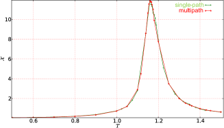
Figure 4: (Color online) Magnetic susceptibility as a function of temperature for $L=10$ in the single–path and multipath approach.

Figure 5: (Color online) Heat capacity as a function of temperature for $L=10$ in the single–path and multipath approach.

From Figs. 2–5, we note that the differences in the thermodynamical characteristic obtained by single–path and multipath approach are negligible.

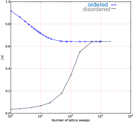
Figure 6: (Color online) Magnetization, calculated starting from both ordered and disordered states, as a function of number of lattice sweeps for $\mathcal{N}=10^{4}$, at $T=1$.

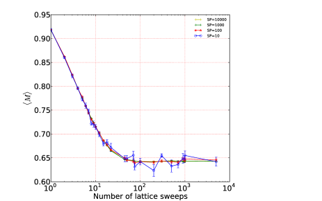
Figure 7: (Color online) Magnetization, calculated starting from ordered state, as a function of number of lattice sweeps for different number of simulation paths, at $T=1$, for $\mathcal{N}=10,100,1000$ and $10000$.

The number of lattice sweeps needed for a lattice to reach it’s representative state (also called burn-in or warm–up phase) is unknown. It depends on many parameters and can vary substantially. Insufficient number of lattice sweeps causes inaccurate simulation results. To overcome this problem for each temperature half of the simulation paths are computed from the random initial state where other half started from the ordered state These two sets are averaged using (7) but results from each half separately. When both halves produce the same result (Figure 6) we can be reasonably certain that it is an accurate value.

Total spin distribution at $T=1$, with $5\times 10^{3}$ lattice sweeps and $10000$ simulation paths is presented in Figure 8. In Figure 8 every path starts from random lattice configuration. From all those measurments magnetization is obtained (see gray line at Figure 6).

However, contrary of that, total spin distributions in Figs 9 and 10 are obtained from multipath simulation where every path started from ordered state. Both sets of measurments, one from Figure 9 and the other one from Figure 10, give the same value of magnetization (blue line in Figure 6).

Multipath approach of the $O(3)$ classical Heisenberg model shows phase transition from the ordered ferromagnetic phase to the paramagnetic phase at temperature $T_{c}=1.442(20)$ (see [7]).

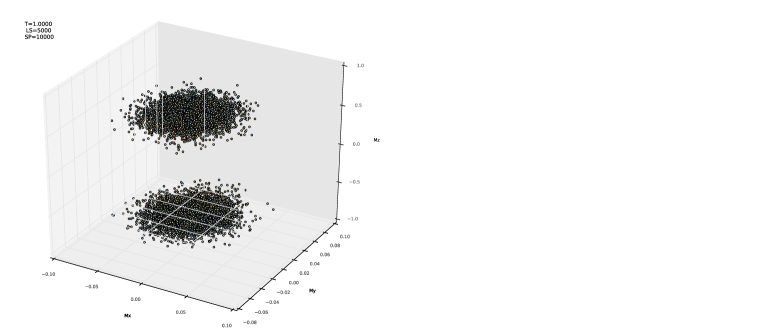
Figure 8: (Color online) Distribution of total spin at $T=1$, for $5\times 10^{3}$ lattice sweeps and $10^{4}$ simulation paths. Every path started from random spin configuration, where both angles $\theta$ and $\varphi$ are taken to be random.

Figure 9: (Color online) Distribution of total spin at $T=1$, for $5\times 10^{3}$ lattice sweeps and $10^{4}$ simulation paths. Every path started from ordered configuration, with $\theta=0$ and $\varphi$ arbitrary.

Figure 10: (Color online) Distribution of total spin at $T=1$, for $5\times 10^{3}$ lattice sweeps and 10000 simulation paths. Every path started from ordered configuration, with $\theta=\pi$ and $\varphi$ arbitrary.

To demonstrate the applicability of multipath approach we examined the thermodynamical properties of classical Heisenberg model and compared it with the results obtained from conventional single–path approach. As expected,the results are in good agreement. The multipath approach produces statistically independent results on which standard statistical methods can be applied [7]. Therefore, it is possible to conduct a ”short simulation” for a quick qualitative analysis (Figure 7), which can be of great importance in research of new models.

References

References

- [1] J. Zinn-Justin, Phase transitions and renormalization group, Oxford University Press, 2007.
- [2] A. P. Young, B. S. Shastry, Theory of the spin dynamics of paramagnetic EuO and EuS, Journal of Physics C: Solid State Physics 15 (21) (1982) 4547.
- [3] R. M. Nowotny, K. Binder, Classical Heisenberg antiferromagnets with nearest and next-nearest neighbor interactions on the face-centered cubic lattice: a model for EuTe?, Zeitschrift für Physik B Condensed Matter 77 (2) (1989) 287–301.
- [4] H. E. Stanley, T. A. Kaplan, High - Temperature Expansions the Classical Heisenberg model, Physical Review Letters 16 (22) (1966) 981–983.
- [5] W. Bialek, A. Cavagna, I. Giardina, T. Mora, E. Silvestri, M. Viale, A. M. Walczak, Statistical mechanics for natural flocks of birds, Proceedings of the National Academy of Sciences 109 (13) (2012) 4786–4791.
- [6] M. D. Leblanc, J. P. Whitehead, M. L. Plumer, Monte Carlo simulations of intragrain spin effects in a quasi-2D Heisenberg model with uniaxial anisotropy, Journal of Physics: Condensed Matter 25 (19) (2013) 196004.
- [7] P. S. Rakic, S. M. Radosevic, P. M. Mali, L. M. Stricevic, Multipath Metropolis Simulation of Classical Heisenberg Model, http://arxiv.org/abs/1305.6758 (2 2014).
- [8] G. F. Newell, E. W. Montroll, On the Theory of the Ising Model of Ferromagnetism, Rev. Mod. Phys. 25 (1953) 353–389.
- [9] S. Jin, A. Sen, A. W. Sandvik, Ashkin-Teller criticality and pseudo-first-order behavior in a frustrated Ising model on the square lattice, Physical Review Letters 108 (4) (2012) 045702.
- [10] W. Selke, L. Shchur, Critical cumulant in two-dimensional anisotropic Ising models, Journal of Physics A: Mathematical and General 38 (44) (2005) L739–L744.
- [11] F. Y. Wu, The Potts model, Rev. Mod. Phys. 54 (1982) 235–268.
- [12] Z. Glumac, K. Uzelac, Yang-Lee zeros and the critical behavior of the infinite-range two- and three-state Potts models, Phys. Rev. E 87 (2013) 022140.
-
[13]
P. S. Rakić, The
Hypermo library [online] (2013).
URL http://bitbucket.org/predrag-rakic/hypermo/ -
[14]
The Centre of Supercomputing of Galicia (CESGA)
[online] (2013).
URL http://www.cesga.es -
[15]
T. Petrić, The tulipko
visualization tool [online] (2013).
URL https://bitbucket.org/iTrustedYOu/tulipko - [16] K. Binder, Finite Size Scaling Analysis of Ising Model Block Distribution Functions, Zeitschrift für Physik B Condensed Matter 43 (2) (1981) 119–140.
- [17] C. Price, N. B. Perkins, Finite-temperature phase diagram of the classical Kitaev-Heisenberg model, Phys. Rev. B 88 (2013) 024410.