Noise Weighting in the Design of Modulators
(with a Psychoacoustic Coder as an Example)

Abstract

A design flow for modulators is illustrated, allowing quantization noise to be shaped according to an arbitrary weighting profile. Being based on FIR NTFs, possibly with high order, the flow is best suited for digital architectures. The work builds on a recent proposal where the modulator is matched to the reconstruction filter, showing that this type of optimization can benefit a wide range of applications where noise (including in-band noise) is known to have a different impact at different frequencies. The design of a multiband modulator, a modulator avoiding DC noise, and an audio modulator capable of distributing quantization artifacts according to a psychoacoustic model are discussed as examples. A software toolbox is provided as a general design aid and to replicate the proposed results.

I Introduction

While often associated to analog to digital (A/D) conversion, modulators are in fact coders that enjoy a wide range of applications. Generally speaking, they exploit a nonlinear feedback architecture (Fig. 1) to translate an analog or high-resolution digital input into a low-resolution high-sample-rate digital signal with minimal loss of fidelity [1]. As a matter of fact, their prevalent commercial deployment is as digital units, namely Digital Modulators [2], used in tasks such as digital to analog (D/A) and digital to digital (D/D) conversion [1], fractional Phase Locked Loops [3], etc.

A key phase in their design is the selection of the Noise Transfer Function (NTF) [4], fundamental to the preservation of information content. This is particularly true for DMs, whose digital nature frees the designer from many limitations. However, the Literature is mostly concerned with analog architectures and many of its NTF considerations are over constrained or not directly applicable to DMs [2].

Recall that the NTF derives from a linear approximation replacing the modulator quantizer with the superposition of a noise signal ($\epsilon(nT)$ in Fig. 1, where $T$ is the sample period). Together with the Classical Model of Quantization (CMQ) [5], this lets the modulator behavior be expressed by two items: the Signal Transfer Function (STF), from input $u(nT)$ to output $x(nT)$, and the NTF, from $\epsilon(nT)$ to $x(nT)$. In principle, full preservation of information is possible if $u(nT)$, passed through the STF, is decoupled in band (i.e., separable by a linear filter) from $\epsilon(nT)$ passed through the NTF. In practice, a full decoupling is never possible. Even if it were, an ideal filter to separate away the quantization noise would not be realistically available [6]. Thus, the designer should select the best possible (good enough) NTF given actual conditions.

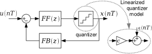
Figure 1: General block diagram of a discrete-time modulator and approximated linear model.

In this paper, a design strategy for the NTF is proposed allowing the quantization noise (including the residual in-band noise) to be shaped according to an arbitrary weighting (cost) profile. This is not possible with conventional flows [5, 7, 8], which merely distinguish between the signal band and out of band frequencies, aiming just at concentrating noise in the latter. While in principle valid for analog modulators too, the proposed strategy is best suited for DMs since it delivers a Finite Impulse Response (FIR) NTF, which may easily require a high order. The work builds on [6] that, owing to the interpretation of DMs as heuristic optimizers for filtered-approximation problems [9, 10], suggests that modulators can be matched to their output/reconstruction filters (as exemplified by the applications in [11, 12]). Here, we introduce a change in perspective illustrating how the same type of optimization can also benefit a wide range of applications where an explicit, tangible filter does not exist but nevertheless there are known reasons for suffering more from some types of noise than from others. To do so, we emphasize by an alternative but equivalent mathematical derivation that even when a filter can be identified only its magnitude response determines the NTF design, so that the response can be reinterpreted as a weighting.

The applicability of the proposed design flow is wide: (i) using on-off weighting functions (1 in the signal band and 0 out of it) it reproduces conventional design methods; (ii) it deals with situations that cannot be easily managed otherwise, such as multiband signals; (iii) most important, it simplifies the management of the sub-ideal behaviors that characterize real world applications, letting the residual in-band noise be concentrated where it can be less harmful and the out-of-band noise be concentrated where the removal can be more efficient.

The paper provides many application examples including the design of a coder for audio applications distributing the residual in-band noise according to a standard psychoacoustic model [13]. Directions are also provided to download open source code meant for the replication of the results in the examples and as a general aid for the DM designer.

II Background

When a modulator such as that in Fig. 1 is linearized, the relationships between $\mathit{NTF}(z)$, $\mathit{STF}(z)$ and the loop filters $\mathit{FF}(z)$, $\mathit{FB}(z)$ are

$$\begin{cases}\mathit{NTF}(z)=\frac{1}{1+c\mathit{FF}(z)\mathit{FB}(z)}\\ \mathit{STF}(z)=\frac{c\mathit{FF}(z)}{1+c\mathit{FF}(z)\mathit{FB}(z)}\end{cases}\begin{cases}\mathit{FF}(z)=\frac{\mathit{STF}(z)}{c\mathit{NTF}(z)}\\ \mathit{FB}(z)=\frac{1-\mathit{NTF}(z)}{\mathit{STF}(z)}\end{cases}$$ (1)

where $c=1$ is customarily assumed. This means that the NTF selection fully determines the modulator whenever the STF is pre-assigned. Typically, specifications want $\mathit{STF}(z)$ to be unitary or at most an integer delay $z^{-d}$ with $d\in\mathbbm{N}$. In the following, $\mathit{STF}(z)$ shall be assumed to be $1$ for simplicity.

CMQ states that uniform quantization can be approximately modeled as the superimposition of noise, white in spectrum, independent from the quantized signal and uniformly distributed within $[\nicefrac{{-\Delta}}{{2}},\nicefrac{{+\Delta}}{{2}}]$, where $\Delta$ is the quantization step. It holds relatively well whenever the modulator input signal is “busy” [5]. With this, the input noise power is $\sigma^{2}_{\epsilon}=\nicefrac{{\Delta^{2}}}{{12}}$, and its Power Spectral Density (PSD) is uniform and equal to $\Psi_{\epsilon}(f)=\nicefrac{{\Delta^{2}}}{{6}}$, with $f$ normalized in $[0,\nicefrac{{1}}{{2}}]$. Consequently, the noise component at the modulator output has a PSD

$$\Psi_{n}(f)=\frac{\Delta^{2}}{6}\left|\mathit{NTF}\left(\mathrm{e}^{\mathrm{i}2\pi f}\right)\right|^{2}.$$ (2)

The NTF choice is subject to some constraints. First of all, the modulator loop cannot be algebraic. Thus, $c\mathit{FF}(z)\mathit{FB}(z)=\nicefrac{{(1-\mathit{NTF}(z))}}{{\mathit{NTF}(z)}}$ must include some delay. This condition can only be satisfied if the NTF impulse response has a unitary zero lag coefficient. Secondly, one must guarantee that the modulator loop is stable. This condition is hard to tackle since it is not sufficient to look at the approximated linear model. However, it is known that a frequent mechanism that can break the modulator operation is the overloading of the quantizer [5]. Thus, a common approach to favor stability consists in limiting the peak gain of the NTF, taking

$$\left\|\mathit{NTF}\right\|_{\infty}=\max_{f\in[0,\frac{1}{2}]}\left|\mathit{NTF}\left(\mathrm{e}^{\mathrm{i}2\pi f}\right)\right|<\gamma$$ (3)

where $\gamma$ is a constant set from the quantizer resolution. Binary quantizers need $\gamma\leq 2$ with $1.5$ being often used. This condition, known as Lee criterion [14] is neither necessary nor sufficient for correct operation, but is empirically known to work well in a large variety of practical cases.

III Noise weighting in the NTF selection

Conventional design flows assume that the NTF can be selected from the input signal properties only. They take the signal band $\mathcal{B}$ as a starting point to deliver an NTF such that the quantization noise is attenuated as much as possible in $\mathcal{B}$, and thus pushed to $[0,\nicefrac{{1}}{{2}}]\setminus\mathcal{B}$, where this complement set is sufficiently large thanks to the Oversampling Ratio (OSR). All these design flows neglect two aspects:

1. no matter how hard they try, they will never succeed in removing all the quantization noise from the signal band, since this would require a brick-wall NTF. Even if the latter could be obtained, no real-world modulator would fully obey to it;

2. even if the whole of the quantization noise could be pushed out of the signal band, it would be impossible to ignore it, since no real world filter would be able to fully remove it.

Furthermore, conventional strategies typically assume that $\mathcal{B}$ is an interval and cannot be easily extended to multi-band cases.

One can immediately see that the way in which the residual in band quantization noise distributes can matter and that the way in which the noise pushed out of band gets distributed is important as well. Actually, these considerations have been clear for a long time. Already in 1997, [15] attempted at designing modulators for audio applications capable to distribute the residual in-band quantization noise so that it could be minimally audible. However, the refinement of these older attempts is somehow limited. More recently, [16] proposed a formal method to minimize the peak values of the in-band residual noise (namely to minimize the maxima of $\left|\mathit{NTF}\left(\mathrm{e}^{\mathrm{i}2\pi f}\right)\right|$). Furthermore, [6] proposed an output filter aware design strategy where the modulator NTF is matched to the filter in charge of removing the out-of-band noise.

Here, we propose the introduction of a cost factor $\nu$ based on a weighting function $w:[0,\nicefrac{{1}}{{2}}]\to\mathbbm{R}^{+}$

$$\nu=\int_{0}^{\frac{1}{2}}\Psi_{n}(f)w(f)\,df$$ (4)

so that the NTF design can be based on its minimization. This lets points (i) and (ii) be flexibly managed. Furthermore, it obviously represents a generalization of conventional design strategies as well as specialized ones like [15], since $w(f)$ can be taken on-off or shaped according to given profiles such as equal-loudness ones [13, 17]. With respect to [6] it can be viewed as change in perspective since the design strategy becomes aware of a cost function, which may not have a corresponding block in the physical architecture of the system.

To deal with the minimization, the NTF needs to be restricted to a FIR form, to guarantee that non-convex expressions, which would be unmanageable, are avoided [6]. A $P$ order NTF (leading to a $P$ order modulator) is described by $P+1$ coefficients $a_{0},\dots,a_{P}$ as in

$$\mathit{NTF}(z)=\sum_{i=0}^{P}a_{i}z^{-i}\ .$$ (5)

This form also guarantees the causality of the modulator filters [6]. From (5), the NTF frequency response is immediately obtained as the Discrete Time Fourier Transform (DTFT) of the coefficients [18] like $\mathit{NTF}\left(\mathrm{e}^{\mathrm{i}2\pi f}\right)=\sum_{i=0}^{P}a_{i}\,\mathrm{e}^{\mathrm{i}2\pi fi}$. Thus,

$$\nu=\frac{\Delta^{2}}{6}\int_{0}^{\frac{1}{2}}\left|\sum_{i=0}^{P}a_{i}\,\mathrm{e}^{\mathrm{i}2\pi fi}\right|^{2}w(f)\,df=\\ \frac{\Delta^{2}}{6}\sum_{i=0}^{P}\sum_{j=0}^{P}a_{i}a_{j}\int_{0}^{\frac{1}{2}}w(f)\,\mathrm{e}^{\mathrm{i}2\pi f(i-j)}\,df.$$ (6)

The latter can be concisely re-expressed in matrix form as $\nu=\frac{\Delta^{2}}{6}\,\boldsymbol{a}^{\mathrm{T}}\boldsymbol{\hat{Q}}\,\boldsymbol{a}$, where the superscript ^T indicates transposition. To do so it is sufficient to let $\boldsymbol{a}=(a_{0},\dots,a_{P})^{\mathrm{T}}$ and $\boldsymbol{\hat{Q}}=(\hat{q}_{i,j})$ be a $(P+1)\times(P+1)$ matrix with entries

$$\hat{q}_{i,j}=\int_{0}^{\frac{1}{2}}w(f)\,\mathrm{e}^{\mathrm{i}2\pi f(i-j)}\,df.$$ (7)

Since $\hat{q}_{i,j}$ only depends on $i-j$, $\boldsymbol{\hat{Q}}$ is Toeplitz. Furthermore, $\hat{q}_{j,i}=\hat{q}^{*}_{i,j}$ where the asterisk indicates conjugation, so that $\boldsymbol{\hat{Q}}$ is Hermitian. With this, $\boldsymbol{a}^{\mathrm{T}}\boldsymbol{\hat{Q}}^{*}\,\boldsymbol{a}=\boldsymbol{a}^{\mathrm{T}}\boldsymbol{\hat{Q}}\,\boldsymbol{a}=\nicefrac{{1}}{{2}}\;\boldsymbol{a}^{\mathrm{T}}\boldsymbol{Q}\,\boldsymbol{a}$, with $\boldsymbol{Q}=\boldsymbol{\hat{Q}}+\boldsymbol{\hat{Q}}^{*}$, where $\boldsymbol{\hat{Q}}^{*}$ is the adjoint of $\boldsymbol{\hat{Q}}$. Thus

$$\nu=(\nicefrac{{\Delta^{2}}}{{3}})\,\boldsymbol{a}^{\mathrm{T}}\boldsymbol{Q}\,\boldsymbol{a}$$ (8)

where $\boldsymbol{Q}$ is a Toepliz symmetric, positive defined real matrix, fully determined by its first row, whose entries are $q_{0,j}=2\Re\left(\int_{0}^{\frac{1}{2}}w(f)\,\mathrm{e}^{-\mathrm{i}2\pi fj}\,df\right)$. Interestingly, by extending $w(f)$ for negative $f$ values, so that $w(-f)=w(f)$, one also has

$$q_{0,j}=\int_{-\frac{1}{2}}^{\frac{1}{2}}w(f)\,\mathrm{e}^{-\mathrm{i}2\pi fj}\,df.$$ (9)

from which $\boldsymbol{Q}$ eventually appears to be defined by the first $P+1$ entries of the Inverse Discrete Time Fourier Transform (IDTFT) of $w(f)$.

Note that the cost factor $\nu$ herein derived is equivalent to that used in [6]. In fact, such paper assumes that an output filter is identifiable after the modulator and aims at matching the modulator design to its features expressed via the impulse response $h_{0},h_{1},h_{2},\dots$. Yet, one can quickly see that matching is optimized via the minimization of a quadratic form based on a matrix whose entries are $q_{j,k}=\sum_{i=-\infty}^{\infty}h_{i-j}h_{i-k}$ [6, Eqn. (17)]. These can be easily recognized as self-correlation entries of the impulse response. The discrete form of the Wiener-Khinchin theorem [18] lets this self-correlation be related to the PSD of the impulse response itself. Thus, in [6] the matching could have been eventually based on the magnitude response of the filter. Here, we change the perspective by re-interpreting the squared magnitude response as an abstract weighting function, to disengage from application frameworks where a tangible output filter is recognizable. The current derivation of $\boldsymbol{Q}$ emphasizes this possibility by doing away with a filter-based notation altogether. Furthermore, it quickly provides an operative, accurate way to get $\boldsymbol{Q}$ from $w(f)$ via the IDTFT operator. Incidentally, note that any attempt at getting $\boldsymbol{Q}$ from the Fast Fourier Transform of samples of $w(f)$ would be prone to artifacts from aliasing.

Once the goal function is established, the optimal NTF coefficients can be determined as in [6, 16]. After $a_{0}$ is set to $1$, the Lee criterion is managed by defining matrices $\boldsymbol{A}$, $\boldsymbol{B}$, $\boldsymbol{C}$ and $\boldsymbol{D}$ such that: $\boldsymbol{A}$ is $P\times P$ with entries $a_{i,j}=\delta_{i,j+1}$ (where $\delta$ is the Kronecker delta); $\boldsymbol{B}$ is a column vector with $P$ entries, all null but the last one set to $1$; $\boldsymbol{C}$ is $(a_{P},a_{P-1},\dots,a_{1})^{\mathrm{T}}$ and $\boldsymbol{D}=(a_{0})$. With this, the Kalman–Yakubovich–Popov (KYP) lemma [19], lets the criterion be re-expressed as the existence of a square symmetric positive defined matrix $\boldsymbol{P}$ such that

$$\begin{pmatrix}\boldsymbol{A}^{\mathrm{T}}\,\boldsymbol{P}\,\boldsymbol{A}-\boldsymbol{P}&\boldsymbol{A}^{\mathrm{T}}\,\boldsymbol{P}\,\boldsymbol{B}&\boldsymbol{C}^{\mathrm{T}}\\ \boldsymbol{B}^{\mathrm{T}}\,\boldsymbol{P}\,\boldsymbol{A}&\boldsymbol{B}^{\mathrm{T}}\,\boldsymbol{P}\,\boldsymbol{B}-\gamma^{2}&\boldsymbol{D}\\ \boldsymbol{C}&\boldsymbol{D}&-1\end{pmatrix}\leq 0$$ (10)

where ‘$\leq$’ is used to state negative semi-definiteness. Altogether, one has a semidefinte program [20] that can be tackled by interior point methods [21].

IV Examples

IV-A Replication of conventional design flows

Conventional design flows typically take as input a modulator type, e.g., Low-Pass (LP) or Band-Pass (BP), and an OSR. These specification can be trivially converted into on-off weightings. For instance, consider the design of an LP modulator with $\mathit{OSR}=64$. This straightforwardly converts into $w(f)$ equal to $1$ for $f<\nicefrac{{1}}{{128}}$ and $0$ otherwise, as in Fig 2a. Fig. 2b shows the magnitude response of a 10${}^{\text{th}}$ order FIR NTF obtained by the proposed approach, and compares it to that of a 2${}^{\text{nd}}$ order NTF obtained by DELSIG’s synthesizeNTF [5]. Obviously, for the FIR based approach the order must be higher. However, the two plots show that the ability to replicate the results of conventional design flows is almost perfect.

-1ex

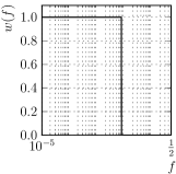
(a)

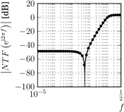
(b)

Figure 2: Sample on-off specification for an LP modulator with $\mathit{OSR}=64$ LABEL:sub@sfig:on-off and corresponding NTF magnitude response LABEL:sub@sfig:on-off-ntf. In LABEL:sub@sfig:on-off-ntf, the solid line is obtained with the proposed method for a 10${}^{\text{th}}$ order FIR NTF, while the dots are obtained with DELSIG’s synthesizeNTF for a 2${}^{\text{nd}}$ order IIR NTF.

IV-B Design of a multiband modulator

The proposed method makes the design of multiband modulators totally consistent with that of single band ones. It is sufficient to take an on-off weighting function that is non-null in multiple frequency intervals. As an example, consider a two band modulator where the bands are $[0,1]\,\mathrm{kHz}$ and $[8,15]\,\mathrm{kHz}$, so that the overall bandwidth is 8 kHz. Assume that the OSR is 8, so that the sample frequency is 128 kHz. The on-off weighting function corresponding to this setup is $w(f)$ equal to $1$ for $f$ in $[0,\nicefrac{{1}}{{64}}]\cup[\nicefrac{{1}}{{8}},\nicefrac{{15}}{{64}}]$ and null elsewhere, as in Fig. 3a. The corresponding NTF obtained by the proposed design method for a 32${}^{\text{th}}$ order FIR NTF is shown in Fig. 3b.

-1ex

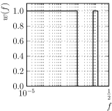
(a)

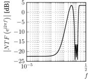
(b)

Figure 3: Sample on-off specification for a multiband modulator with $\mathit{OSR}=8$ LABEL:sub@sfig:on-off-multi and corresponding NTF magnitude response LABEL:sub@sfig:on-off-multi-ntf obtained designing the NTF with the proposed method for a 32${}^{\text{nd}}$ order FIR NTF.

Note that multiband signals cannot generally be managed by conventional design flows. For instance, none of the NTF design routines in the DELSIG toolbox can straightforwardly deal with this case. Only very recent design approaches such as [16, 6] are suitable for this task. For what concerns [6], some comparison is provided in the next Section IV-C.

IV-C Design of a modulator capable of optimally dealing with an imperfect filter for the removal of quantization noise

This case is the one tackled in [6]. It is reported precisely to illustrate how the optimization procedures is ultimately the same. Suppose that a DM D/A setup deals with signals defined in a [0,1] kHz band and that the reconstruction filter is a mere 1${}^{\text{st}}$ order Butterworth unit with cut-off at 1 kHz. Let the OSR be 64. This relatively large value lets one approximate the reconstruction filter in discrete time with good precision as $H(z)=12.12\times 10^{-3}\;\nicefrac{{(z+1)}}{{(z-0.976)}}$. The residual quantization noise after the reconstruction filter can be estimated as in Fig. 4, where a reference signal $\hat{y}(nT)$, obtained by filtering $u(nT)$ through the STF and $H(z)$ is subtracted from the actual output of the reconstruction filter $y(nT)$ to give $\hat{\epsilon}(nT)$. Since the paths through the STF and $H(z)$ elide each other, the residual noise is $\epsilon(nT)$ filtered through the NTF and $H(z)$. Thus, its power is

$$\sigma^{2}_{\hat{\epsilon}}=\int_{0}^{\frac{1}{2}}\Psi_{n}(f)\left|H\left(\mathrm{e}^{\mathrm{i}2\pi f}\right)\right|^{2}\,df$$ (11)

This is formally analogous to Eqn. (4) when $w(f)=\left|H\left(\mathrm{e}^{\mathrm{i}2\pi f}\right)\right|^{2}$. Unsurprisingly, the non-ideal reconstruction filter determines a noise weighting equivalent to its magnitude response. However, from a practical point of view, the computation of the optimal modulator NTF based on the IDTFT operator is more efficient and accurate than that proposed in [6], the latter being based on a computation practiced in the time domain from the filter impulse response. For the sake of comparison, Fig. 5b also shows a reference NTF obtained by DELSIG’s synthesizeNTF. As in [6], the value of $\sigma^{2}_{\hat{\epsilon}}$ obtained by the proposed method is almost 5 dB better than the reference one.

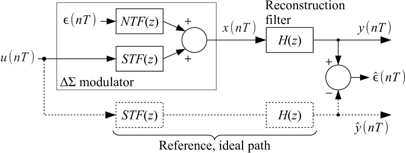
Figure 4: Evaluation of the residual noise after the application of a reconstruction filter.

-1ex

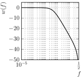
(a)

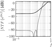
(b)

Figure 5: Noise weighting function for an LP modulator with $\mathit{OSR}=64$ and a 1${}^{\text{st}}$ order Butterworth reconstruction filter LABEL:sub@sfig:lp and corresponding optimal NTF magnitude response LABEL:sub@sfig:lp-ntf for a 10${}^{\text{th}}$ order FIR NTF (solid). For comparison, a 4${}^{\text{th}}$ order conventional NTF obtained with DELSIG is also shown (dashed).

IV-D Design of a modulator with reduced dc noise

In some testing or sensing applications, excitations are obtained by storing an off-line generated sequence into a memory and playing it through a LP filter. Some of these applications are particularly sensitive to dc errors, so that one may want a particularly low noise at low frequency values. The proposed method makes it quite easy to achieve this result by starting with an on-off noise weighting function (like in Fig. 2a) and then raising it at low frequencies. Fig. 6a shows how this can be done together with the outcome in terms of NTF. Fig 6b shows that the method works, providing the actual PSD of the shaped quantization noise, as obtained from time-domain simulations run on the nonlinear modulator model.

-1ex

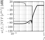
(a)

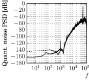
(b)

Figure 6: In LABEL:sub@sfig:on-off+dc: noise weighting function (thin line) and NTF magnitude response (thicker) for an LP modulator capable of providing reduced noise close to dc (both solid). Data from the case in Sec. IV-A provided for comparison (dashed). OSR is 64 and the NTF FIR order is 32. In LABEL:sub@sfig:on-off+dc-pds: the corresponding PSD of the shaped quantization noise, as obtained from time-domain simulations.

IV-E Design of a psychoacoustically optimal coder for audio

DMs can be used as coders in audio applications in view of highly efficient switched-mode amplification [22] or even to prepare data for certain storage formats [23]. In these applications, one wants the in-band residual quantization noise to be minimally audible. The way in which the ear reacts to sound pressure levels is extremely complex since in human evolution the cochlea has learned to be most sensitive to the sounds most important for survival. Such complexity is today captured by psychoacoustic models, commonly based on equal-loudness contours such as those in ISO 226 [13]. ISO tables a family of functions $L_{p}(f;L_{N})$, obtained from experiments over a multitude of listeners and parametrized over a perceived sound loudness $L_{N}$. At each characterized frequency, the actual acoustic power (sound pressure level) necessary to get $L_{N}$ is returned. When a listener is exposed to a sound, the overall perception can be quantified by integrating the sound PSD multiplied by a weighting profile obtained from $L_{p}(f;L_{N})$ (approximately as its inverse, although corrections accounting for nonlinear effects, limited reach at high frequency and acoustic field features are commonly applied too [17]). Specific weightings have been developed for the significant case where the sound is a spread-spectrum, low-level noise, a notable one being the F-weighting, based on $L_{P}(f;15\,\mathrm{phon})$, and characterized as an analytic expression in [17]. The present design flow makes it easy to directly exploit weightings as the F one for the design of DMs.

Note that in principle also the magnitude response of every unit between the coder and the hear (e.g. filters, amplifiers, loudspeakers), should be considered. However, common weightings are already so steep at their edges (below $20\,\mathrm{Hz}$ and above 16 kHz), that unless pathological components are used for these units, the influence of their band limitations on noise perception is negligible. Here, we use the F-weighting as $w(f)$, since this also favors comparison to previous results in the Literature.

Fig 7a shows $w(f)$ together with a sample optimal NTF obtained with our design flow and another one obtained with the approach described in [15] to design psychoacoustically optimal DMs. Fig 7b shows the perceived noise spectra obtained by time-domain simulations in the two cases. Clearly the NTFs are quite different. This is due to many reasons. The most evident one is that [15] follows conventional design methods [5], just plugging onto them a step where NTF zeros are adjusted on the unit circle until the perceived noise PSD is made as flat as possible in the signal band. Consequently, the NTF ends up having a number of valleys proportional to the modulator order. In our approach, except for very low orders, the NTF ends up always having as many valleys as there are peaks in the weighting profile. Furthermore, because our approach is less constrained, it succeeds better in lowering the NTF where this is important for the perceived SNR, namely where the weighting profile (normalized to peak slightly above 0 dB) and the NTF intersect.

-1ex

(a)

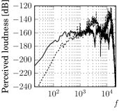
(b)

Figure 7: In LABEL:sub@sfig:psycho-ntf: noise weighting function (thin line) and NTF magnitude response (thicker) for a psychoacoustically optimal audio coder based on the F-Weighting (30${}^{\text{th}}$ order). The NTF from a 3${}^{\text{rd}}$ order DM designed with the approach in [15] is provided for comparison (dashed). OSR is 64. In LABEL:sub@sfig:on-off+dc-pds: the corresponding perceived loudness level of quantization noise as a function of frequency.

V Conclusions

A design flow for modulators has been illustrated, allowing quantization noise to be shaped according to an arbitrary weighting profile. It is best suited for DMs in applications where quantization noise (including the residual in-band noise) is known to have a different impact at different frequencies. An implementation is available at http://pydsm.googlecode.com as part of an open source toolbox. This is coded in Python/Scipy [24] and based on the CVXOPT/CVXPY optimization core [21]. It is easy to install, can run on Linux and Windows and only depends on free software. It can be used to replicate the many examples in this paper or as a general design aid.

References

- [1] F. Harris, “Sigma-delta converters in communication systems,” in Wiley Encyclopedia of Telecommunications, J. G. Proakis, Ed. John Wiley & Sons, Inc., 2003, vol. IV, pp. 2227–2247.
- [2] S. Pamarti, J. Welz, and I. Galton, “Statistics of the quantization noise in 1-bit dithered single-quantizer digital delta-sigma modulators,” IEEE Trans. Circuits Syst. I, vol. 54, no. 3, pp. 492–503, Mar. 2006.
- [3] P.-E. Su and S. Pamarti, “Fractional-n phase-locked-loop-based frequency synthesis: A tutorial,” IEEE Trans. Circuits Syst. II, vol. 56, no. 12, pp. 881–885, Dec. 2009.
- [4] S. R. Norsworthy, R. Schreier, and G. C. Temes, Eds., Delta-Sigma Data Converters: Theory, Design, and Simulation. Wiley-IEEE Press, 1996.
- [5] R. Schreier and G. C. Temes, Understanding Delta-Sigma Data Converters. Wiley-IEEE Press, 2004.
- [6] S. Callegari and F. Bizzarri, “Output filter aware optimization of the noise shaping properties of modulators via semi-definite programming,” IEEE Trans. Circuits Syst. I, vol. 60, no. 9, pp. 2352–2365, Sep. 2013.
- [7] J. G. Kenney and L. R. Carley, “Design of multibit noise-shaping data converters,” Analog Integrated Circuits and Signal Processing, vol. 3, pp. 259–272, 1993.
- [8] R. Schreier, The Delta-Sigma Toolbox, Analog Devices, 2011, release 7.4, also known as “DELSIG”. [Online]. Available: http://www.mathworks.com/matlabcentral/fileexchange/
- [9] S. Callegari, F. Bizzarri, R. Rovatti, and G. Setti, “On the approximate solution of a class of large discrete quadratic programming problems by modulation: the case of circulant quadratic forms,” IEEE Trans. Signal Process., vol. 58, no. 12, pp. 6126–6139, Dec. 2010.
- [10] F. Bizzarri and S. Callegari, “A heuristic solution to the optimisation of flutter control in compression systems (and to some more binary quadratic programming problems) via modulation circuits,” in Proc. of ISCAS’10, Paris, FR, May 2010.
- [11] S. Callegari and F. Bizzarri, “Should modulators used in ac motor drives be adapted to the mechanical load of the motor?” in Proceedings of IEEE ICECS 2012, Seville (ES), Dec. 2012, pp. 849–852.
- [12] F. Bizzarri, S. Callegari, and G. Gruosso, “Towards a nearly optimal synthesis of power bridge commands in the driving of AC motors,” in Proceedings of ISCAS 2012, Seoul, May 2012, pp. 2119–2122.
- [13] Acoustics — Normal equal-loudness-level contours, ISO Std. 226, Rev. 2, Aug. 2003.
- [14] W. L. Lee, “A novel high order interpolative modulator topology for high resolution oversampling A/D converters,” Master’s thesis, Massachussets Institute of Technology, 1987.
- [15] C. Dunn and M. Sandler, “Psychoacoustically optimal sigma delta modulation,” Journal of the Audio Engineering Society (AES), vol. 45, no. 4, pp. 212–223, Apr. 1997.
- [16] M. Nagahara and Y. Yamamoto, “Frequency domain Min-Max optimization of noise-shaping Delta-Sigma modulators,” IEEE Trans. Signal Process., vol. 60, no. 6, pp. 2828–2839, Jun. 2012.
- [17] R. A. Wannamaker, “Psychoacoustically optimal noise shaping,” Journal of the Audio Engineering Society, vol. 40, no. 7/8, p. 611–620, 1992.
- [18] A. V. Oppenheim and R. W. Schafer, Discrete-Time Signal Processing. Prentice-Hall, 1989.
- [19] T. Iwasaki and S. Hara, “Generalized KYP lemma: Unified frequency domain inequalities with design applications,” IEEE Trans. Autom. Control, vol. 50, no. 1, pp. 41–59, Jan. 2005.
- [20] S. Boyd, L. El Ghaoui, E. Feron, and V. Balakrishnan, Linear Matrix Inequalities in System and Control Theory, ser. SIAM studies in applied mathematics. Philadelphia: SIAM, 1994, vol. 15.
- [21] M. Andersen, J. Dahl, Z. Liu, and L. Vandenberghe, “Interior-point methods for large-scale cone programming,” in Optimization for Machine Learning, ser. Neural Information Processing series, S. Sra, S. Nowozin, and S. J. Wright, Eds. MIT Press, Sep. 2011, ch. 3, pp. 55–84. [Online]. Available: http://www.ee.ucla.edu/~vandenbe/publications/mlbook.pdf
- [22] E. Gaalaas, “Class D audio amplifiers: What, why, and how,” Analog Dialogue, vol. 40, no. 6, pp. 1–7, Jun. 2006.
- [23] D. Reefman and P. Nuijten, “Why Direct Stream Digital is the best choice as a digital audio format,” in Proc. of the 110th Convention of the Audio Engineering Society, 2001.
- [24] T. E. Oliphant, “Python for scientific computing,” IEEE Comput. Sci. Eng., vol. 9, no. 3, pp. 10–20, May 2007.