Taming Rogue waves in Vector BECs

Abstract

Using Gauge transformation method, we generate rogue waves for the two component Bose Einstein Condensates (BECs) governed by the symmetric coupled Gross-Pitaevskii (GP) equations and study their dynamics. We also suggest a mechanism to tame the rogue waves either by manipulating the scattering length through Feshbach resonance or the trapping frequency, a new phenomenon not witnessed in the domain of BEC, we believe that these results may have wider ramifications in the management of rogons.

I Introduction

Rogue waves are nonlinear single oceanic waves of extremely large amplitude, much higher than the average wave crests around them and are localized both in space and time. Similar to the properties of the solitary waves, rogue waves are also known as ’rogons’ if they reappear virtually unaffected in size or shape shortly after their interactions [1]. Rogue waves have caused tremendous havoc and have contributed to several maritime disasters[2]. In contrast to tsunamis [3] which can be predicted hours (sometimes days) in advance, the danger of oceanic rogue waves is that they appear from nowhere and disappear without even a trace[4].

Eventhough their existence has now been confirmed by several observations, the grim reality is that their generating mechanism is not yet fully understood. The recent studies argue that they arise due to modulation instability [5,6,7], and their occurence has been reported in optics [8], plasma [9] and Bose-Einstein condensates (BECs)[10]. To date, several nonlinear partial differential equations derived from different branches of physics have been shown to admit rogue waves. Among these, the nonlinear Schrodinger(NLS) equation represents the most elegant model to describe rogue waves. Recently, using NLS equation, generating mechanism for multi rogue waves has been proposed [11,12]. The collision of two or more Akhmediev breathers (ABs) resulting from the modulation instability can lead to rogue waves in these systems [12]. At the same time, the discrete integrable systems like generalized Ablowitz-Ladik-Hirota (ALH) lattice with variable coefficients supports the nonautonomous discrete rogue solutions [13]. Since the lifetime of rogue waves is very short, their systematic investigation is very complicated. Penetrating deep into the domain of rogue wave not only helps in understanding their dynamics, but also in controlling their size and lifetime for technological applications, particularly in the realm of nonlinear optics and BECs.

The recent theoretical investigations predict that the rogue wave phenomenon can be observed in integrable multicomponent systems like Manakov model [14], spinor F=1 condensates [15] etc. and have also confirmed the existence of new type of bright- dark-rogue wave solutions. The possible mechanism for the formation of rogue waves in the two-dimensional coupled NLS equations describing the nonlinearly interacting two-dimensional waves in deep water has also been proposed [16-17]. The numerical study on the two-component BECs with variable scattering lengths shows that rogue wave solutions generated by phase and/or density engineering can exist only for certain combinations of the nonlinear coefficients describing two-body interactions [18]. Motivated by these observations, in this paper, we identify a simple mechanism to generate and control the evolution of rogue waves in vector BECs. It should be mentioned that even though rogue waves have been manipulated in nonlinear optics [12,19] and BECs [20], their observation in vector BECs characterized by the symmetric coupled Gross-Pitaevskii (GP) equation has not yet been fully understood. In this paper, we generate rogue waves for the vector BECs governed by the coupled GP equation and manipulate either the scattering length through Feshbach resonance or the trapping frequency to tame them, a new phenomenon not observed in the territory of BECs.

II Theoretical Model and Lax pair

Considering a spinor BEC comprising of two hyperfine states $|F=1,m_{f}=-1>$ and $|F=1,m_{f}=1>$ of the same atom, say ${}^{87}Rb$ [21] confined at different vertical positions by parabolic traps, the dynamics in the mean field approximation is described by the coupled dimensionless GP equation [22] of the following form (for cigar shaped BECs)

$$i\psi_{1t}+\psi_{1xx}+2\eta(t)(|\psi_{1}|^{2} + |\psi_{2}|^{2})\psi_{1}+\lambda(t)^{2}x^{2}\psi_{1}$$ (1)

$$+ iG(t)\psi_{1}=0,$$

$$i\psi_{2t}+\psi_{2xx}+2\eta(t)(|\psi_{1}|^{2} + |\psi_{2}|^{2})\psi_{2}+\lambda(t)^{2}x^{2}\psi_{2}$$ (2)

$$+ iG(t)\psi_{2}=0,$$

where,$\psi_{j}$(j=1,2) represents the order parameter of the condensates, $\eta(t)$ is the temporal scattering length, $\lambda(t)$ the trap frequency and $G(t)$ accounts for the feeding of atoms (loss/gain) from the thermal cloud. The above coupled GP equation has already been investigated [23,24] and the collisional dynamics of bright solitons has been studied.

Eqs. (1),(2) admit the following Lax pair

$$\Phi_{x}=Q_{1}\Phi$$ (3)

$$\Phi_{t}=Q_{2}\Phi$$ (4)

and

$$Q_{1}=\left(\begin{array}[]{ccc}-i\zeta(t)&q_{1}&q_{2}\\ -q_{1}^{*}&i\zeta(t)&0\\ -q_{2}^{*}&0&i\zeta(t)\\ \end{array}\right),$$ (5)

$$Q_{2}=\left(\begin{array}[]{ccc}Q_{2}(11)&Q_{2}(12)&Q_{2}(13)\\ Q_{2}(21)&Q_{2}(22)&Q_{2}(23)\\ Q_{2}(31)&Q_{2}(32)&Q_{2}(33)\\ \end{array}\right),$$ (6)

where

$$Q_{2}(11) = -2i\zeta(t)^{2}+2\zeta(t)i\Gamma(t)x+i(|q_{1}|^{2}+|q_{2}|^{2})$$

$$Q_{2}(12) = 2\zeta(t)q_{1}+i(q_{1x}+2i\Gamma(t)xq_{1})$$

$$Q_{2}(13) = 2\zeta(t)q_{2}+i(q_{2x}+2i\Gamma(t)xq_{2})$$

$$Q_{2}(21) = -2\zeta(t)q_{1}^{*}+i(q_{1x}^{*}-2i\Gamma(t)xq_{1}^{*})$$

$$Q_{2}(22) = 2i\zeta(t)^{2}-2\zeta(t)i\Gamma(t)x-i|q_{1}|^{2}$$

$$Q_{2}(23) = -iq_{2}q_{1}^{*}$$

$$Q_{2}(31) = -2\zeta(t)q_{2}^{*}+i(q_{2x}^{*}-2i\Gamma(t)xq_{2}^{*})$$

$$Q_{2}(32) = -iq_{2}^{*}q_{1}$$

$$Q_{2}(33) = 2i\zeta(t)^{2}-2i\zeta(t)\Gamma(t)x-i|q_{2}|^{2}$$

$$q_{1}(x,t) = \sqrt{\eta(t)}e^{(-i\Gamma(t)x^{2}/2)}\psi_{1}(x,t),$$ (7)

$$q_{2}(x,t) = \sqrt{\eta(t)}e^{(-i\Gamma(t)x^{2}/2)}\psi_{2}(x,t).$$ (8)

In eqs (3,4), $\Phi$ represents the eigenfunction denoted by $(\phi_{1},\phi_{2},\phi_{3})^{T}$ while $(Q_{1},Q_{2})$ denotes the Lax operators described by $(3\times 3)$ matrices while $\zeta(t)$ represents the nonisospectral parameter obeying the following equation

$$\zeta(t)=\mu e^{(-2\int\Gamma(t)dt)}.$$ (9)

In the above equation, $\mu$ is a complex constant and $\Gamma(t)$ is an arbitrary function of time. The compatibility condition $Q_{1t}-Q_{2x}+[Q_{1},Q_{2}]=0$ generates eqs.(1) and (2) with the following constraints

$$G(t)=\Gamma(t)+\frac{1}{2}\frac{\eta^{\prime}(t)}{\eta(t)},\\$$

and

$$\lambda(t)^{2}=\Gamma(t)^{2}+(\Gamma~{}^{\prime}(t)/2).$$ (10)

subject to the integrability condition

$$\lambda(t)^{2}=G(t)^{2}+\frac{1}{2}\frac{\eta^{\prime}(t)^{2}}{\eta(t)^{2}}-G(t)\frac{\eta^{\prime}(t)}{\eta(t)}+\frac{1}{2}G^{\prime}(t)-\frac{1}{4}\frac{\eta^{\prime\prime}(t)}{\eta(t)}.$$ (11)

To obtain the exact solution of eqs (1, 2), we introduce the following dependent variable transformation

$$\psi_{1}(x,t)=\Lambda(x,t)U(X,T),$$ (12)

$$\psi_{2}(x,t)=\Lambda(x,t)V(X,T),$$ (13)

with the coordinates governed by the following equations

$$X = \sqrt{2}r_{0}\eta(t)x-2\sqrt{2}br_{0}^{3}\int\eta(t)^{2}dt$$ (14)

$$T = r_{0}^{2}\int\eta(t)^{2}dt$$ (15)

and

$$\Lambda(x,t)=\sqrt{2r_{0}^{2}\eta(t)}e^{i(-\frac{\eta(t)_{t}}{2\eta(t)}x^{2}+2br_{0}^{2}\eta(t)x-2b^{2}r_{0}^{4}\int\eta(t)^{2}dt)}$$ (16)

where $r_{0}$ and $b$ are arbitrary constants so that eqs. (1,2) reduce to the celebrated Manakov model.

III Construction of Rogue waves

To construct rogue waves, we start from the following nonzero plane wave solution as the seed solution given by

$$\psi_{1}[0]=c_{1}exp[i\theta_{1}],\psi_{2}[0]=c_{2}exp[i\theta_{2}],$$ (17)

where

$$\theta_{1}=g_{1}x+(2c_{1}^{2}+2c_{2}^{2}-g_{1}^{2})t$$ (18)

$$\theta_{2}=g_{2}x+(2c_{1}^{2}+2c_{2}^{2}-g_{2}^{2})t$$ (19)

Feeding the above seed solution into the Lax-pair governed by eqs (3,4), we obtain

$$\Phi_{1x}=(MQ_{1}M^{-1}+M_{x}M^{-1})\Phi_{1}=\hat{Q_{1}}\Phi_{1}$$

$$\Phi_{1t}=(MQ_{2}M^{-1}+M_{t}M^{-1})\Phi_{1}=\hat{Q_{2}}\Phi_{1}$$

where the iterated eigenfunction $\Phi_{1}=M\Phi,M=diag[exp[-\frac{i}{3}(\theta_{1}+\theta_{2})],exp[\frac{i}{3}(2\theta_{1}-\theta_{2})],exp[\frac{i}{3}(\theta_{1}+\theta_{2})]]$ with

$$\hat{Q_{1}}=\left(\begin{array}[]{ccc}\chi_{11}&c_{1}&c_{2}\\ -c_{1}&\chi_{22}&0\\ -c_{2}&0&\chi_{33}\\ \end{array}\right),$$ (20)

$$\hat{Q_{2}}=i\hat{Q_{1}}^{2}-[\frac{2}{3}(g_{1}+g_{2})-2\zeta_{1}]\hat{Q_{1}}+mI$$ (21)

$$\chi_{11}=-2i\zeta_{1}-\frac{i}{3}(g_{1}+g_{2})$$

$$\chi_{22}=i\zeta_{1}-\frac{i}{3}(2g_{1}-g_{2})$$

$$\chi_{33}=i\zeta_{1}+\frac{i}{3}(2g_{2}-g_{1})$$

and the new parameter
$m=2i\zeta_{1}^{2}+\frac{2i}{3}(c_{1}^{2}+c_{2}^{2}+\frac{2i}{9}(g_{1}^{2}-g_{1}g_{2}+g_{2}^{2})+\frac{2i\zeta_{1}}{3}(g_{1}+g_{2})$.

In order to look for the rational solutions, we choose a new parameter $\sigma=g_{2}+3\zeta_{1R},g_{1}=g_{2}-2\sigma,c_{1}=c_{2}=2\sigma$ where $g_{2}$ and $\zeta_{1R}$ are arbitrary real numbers. The fundamental solution matrix for Lax pair equations at $\zeta(t)=\zeta_{1}$ and $\psi=\psi_{j}[0](j=1,2)$ are $\Phi=M^{-1}\Theta$ where

$$\Theta=\left(\begin{array}[]{ccc}\phi_{11}&4\sigma^{2}\nu+2\sqrt{3}\sigma&4\sigma\\ \phi_{21}&-2(\sqrt{3}-i)\nu-2\sigma&-2\sigma^{2}(\sqrt{3}-i)\\ \phi_{31}&\phi_{22}^{*}&\phi_{23}^{*}\\ \end{array}\right)$$ (22)

with

$$\phi_{11} = 4\sigma^{2}(\nu+2it)+4\sqrt{3}\sigma\nu+2$$

$$\phi_{21} = -2(\sqrt{3}-i)\sigma^{2}(\nu^{2}+2it)-4\sigma\nu$$

$$\phi_{31} = -2(\sqrt{3}+i)\sigma^{2}(\nu^{2}+2it)-4\sigma\nu$$

and $\nu=x+2\sqrt{3}(\sigma-i\sqrt{3}\zeta_{1R})it$. To obtain the rational solution of the coupled GP equation, we exploit the gauge transformation approach [25] employing the following transformation

$$\psi_{1}[1]=\psi_{1}[0]-2i(\zeta_{1}-\bar{\zeta}_{1})\frac{\phi_{1}\phi_{2}^{*}}{|\phi_{1}|^{2}+|\phi_{2}|^{2}+|\phi_{3}|^{2}}$$

$$\psi_{2}[1]=\psi_{2}[0]-2i(\zeta_{1}-\bar{\zeta}_{1})\frac{\phi_{1}\phi_{3}^{*}}{|\phi_{1}|^{2}+|\phi_{2}|^{2}+|\phi_{3}|^{2}}$$

The explicit forms of the first order rogue wave solution have the following form

$$\psi_{1} = \sqrt{\frac{2}{\eta(t)}}\varepsilon_{1}^{(1)}\beta(t)\Big{[}-1-i\sqrt{3}+a\Big{]}\times$$ (24)

$$\exp[i\theta_{1}-\xi_{1}+\Gamma(t)x^{2}/2],$$

$$\psi_{2} = \sqrt{\frac{2}{\eta(t)}}\varepsilon_{1}^{(2)}\beta(t)\Big{[}-1-i\sqrt{3}+a\Big{]}\times$$ (25)

$$\exp[i\theta_{2}-\xi_{1}+\Gamma(t)x^{2}/2]$$

where $a=f_{1}/f_{2}$

$$f_{1} = -6\delta\sigma\sqrt{3}-36t\sigma^{2}\sqrt{3}-3+i(36t\sigma^{2}+6\delta\sigma+5\sqrt{3}),$$

$$f_{2} = 12\sigma^{2}\delta^{2}+8\delta\sigma\sqrt{3}+144t^{2}\sigma^{4}+5$$

where $\delta=x+6\zeta_{1R}t$. The gauge transformation approach [25] can be easily extended to generate multi rogue wave solution. For example, the second order rogue wave solution has the following form

$$\psi_{1} = \sqrt{\frac{2}{\eta(t)}}\varepsilon_{1}^{(1)}\beta(t)\Big{[}-1-i\sqrt{3}+a1\Big{]}\times$$ (26)

$$\exp[i\theta_{1}-\xi_{1}+\Gamma(t)x^{2}/2]$$

$$\psi_{2} = \sqrt{\frac{2}{\eta(t)}}\varepsilon_{1}^{(1)}\beta(t)\Big{[}-1-i\sqrt{3}+a2\Big{]}\times$$ (27)

$$\exp[i\theta_{1}-\xi_{1}+\Gamma(t)x^{2}/2]$$

where,

$$a_{1} = \frac{J_{1}+iK_{1}}{D}$$

$$a_{2} = \frac{J_{2}+iK_{2}}{D}$$

$$J_{1}= - 864\sqrt{3}\sigma^{6}t^{3}-144\sqrt{3}\sigma^{5}\delta t^{2}-72\sqrt{3}\sigma^{4}\delta^{2}t-216\sigma^{4}t^{2}$$

$$- 12\sqrt{3}\sigma^{3}\delta^{3}-144\sigma^{3}\delta t-18\sigma^{2}\delta^{2}-12\sqrt{3}\sigma^{2}t+3$$

$$J_{2}= + 864\sqrt{3}\sigma^{6}t^{3}-144\sqrt{3}\sigma^{5}\delta t^{2}+72\sqrt{3}\sigma^{4}\delta^{2}t-216\sigma^{4}t^{2}$$

$$- 12\sqrt{3}\sigma^{3}\delta^{3}+144\sigma^{3}\delta t-18\sigma^{2}\delta^{2}+12\sqrt{3}\sigma^{2}t+3$$

$$K_{1}= + 864\sigma^{6}t^{3}+144\sigma^{5}\delta t^{2}+72\sigma^{4}\delta^{2}t+312\sqrt{3}\sigma^{4}t^{2}+12\sigma^{3}\delta^{3}$$

$$+ 96\sqrt{3}\sigma^{3}\delta t+18\sqrt{3}\sigma^{2}\delta^{2}+108\sigma^{2}t+12\sigma\delta+\sqrt{3}$$

$$K_{2}= + 864\sigma^{6}t^{3}-144\sigma^{5}\delta t^{2}+72\sigma^{4}\delta^{2}t-312\sqrt{3}\sigma^{4}t^{2}-12\sigma^{3}\delta^{3}$$

$$+ 96\sqrt{3}\sigma^{3}\delta t-18\sqrt{3}\sigma^{2}\delta^{2}+108\sigma^{2}t-12\sigma\delta-\sqrt{3}$$

$$D= + 1728\sigma^{8}t^{4}+384\sqrt{3}\sigma^{5}\delta t^{2}+12\sigma^{4}\delta^{4}+432\sigma^{4}t^{2}$$

$$+ 16\sqrt{3}\sigma^{3}\delta{3}+24\sigma^{2}\delta^{2}+4\sqrt{3}\sigma\delta+1$$

where $\eta(t)=2\sigma f(t)$, $\alpha(t)=\alpha_{0}\sigma\exp[-2\int\Gamma(t)dt]$, $\beta(t)=\beta_{0}\sigma\exp[-2\int\Gamma(t)dt]$.

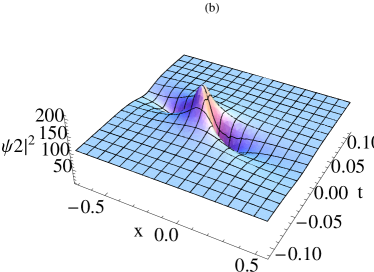
Figure 1: Density profiles of rogue waves for $\eta(t)=0.0006$, $g_{2}=0,e_{1}=0.1,\Gamma(t)=0.01t,f(t)=0.001$

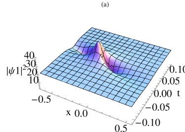
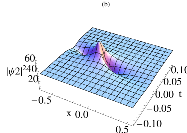
Figure 2: Taming of the rogue waves by manipulating the scattering length for $\eta(t)=0.006$ and $f(t)=0.01$ with the other parameters as in fig 1.

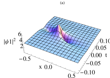
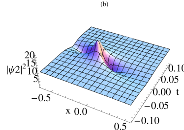
Figure 3: Stabilization of rogue waves for $\eta(t)=0.06$ and $f(t)=0.1$ with the other parameters as in fig 1.

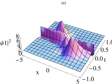
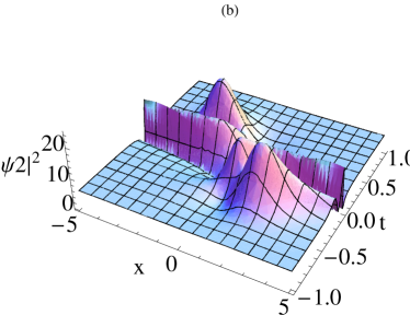
Figure 4: Density profiles of two rogue waves for $\eta(t)=0.12t$, $f(t)=0.05t$ $g_{2}=0.9,e_{1}=0.1,$ and $\Gamma(t)=0.1t,$

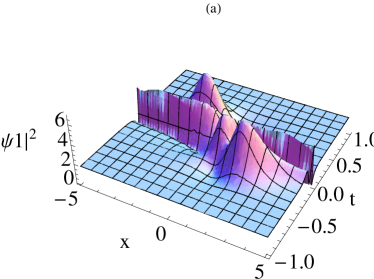
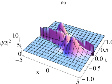
Figure 5: Stabilization of two rogue waves by manipulating the time dependent scattering length for $\eta(t)=0.168t$ and $f(t)=0.07t$ with the other parameters as in fig 4

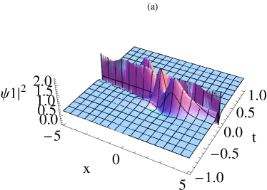
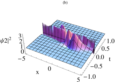
Figure 6: Stabilization of two rogue waves by finetuning the time dependent scattering length for $\eta(t)=0.36t$ and $f(t)=0.15t$ with the other parameters as in fig 4

IV Stabilization of Rogue waves

Fig.(1) shows the density profiles of first order rogue waves governed by the scattering length for $\eta(t)=0.0006$ and $f(t)=0.001$. It is obvious from fig (1) that the density of rogue waves is enormous which means that it would collapse or disappear in a short interval of time during time evolution. To stabilize (reduce the density) the rogue waves and thereby increase its lifespan, we harness the fact that their densities $|\psi_{j}|^{2}(j=1,2)$ is inversely proportional to the scattering length $\eta(t)$ (of course, $\eta(t)$ varies directly with $f(t)$). Hence, we manipulate (increase) the scattering length $\eta(t)$ through Feshbach resonance suitably to stabilize the first order rogue waves as shown in fig(2). Rogue waves can be stabilized further for $\eta(t)=0.06$ and $f(t)=0.1$ as shown in fig(3). This process of stabilizing the amplitude of rogue waves and thereby increasing the lifetime is called ’Taming’. Fig (4) shows the density profile of second order rogue waves for time dependent scattering lengths $\eta(t)=0.12t$ and $f(t)=0.05t$. Again, one can tame the rogue waves further by fine-tuning the time dependent scattering lengths as shown in figs (5) and (6). From figs(4-6), one understands that the density of the rogue waves decreases by finetuning the time dependent scattering lengths. This means that one can delay the inevitable (the collapse or disappearance of the condensates) by manipulating the time dependent scattering lengths as well. In addition, the fact that it stretches over a finite interval of time compared to figs(1-3) means that one finally ends up increasing the lifespan of BECs.

It should also be mentioned that the trapping frequency $\lambda(t)$ which is related to $\Gamma(t)$ by virtue of eqn. (10) can also suitably changed to tame rogue waves. Fig (7) shows the density profile of second order rogue waves for periodically varying scattering lengths $\eta(t)=2cos(0.15t)$ and $f(t)=cos(0.15t)$ and fig.8 depicts the corresponding contour plot. The contour plot shown in fig.9 depicts the time evolution of second order rogue waves shown in fig.8 by maneuvering the trap frequency $\Gamma(t)=0.1t$. Further evolution of the second order rogue waves shown in fig.10 shows that one can certainly enhance the lifespan of the rogue waves by manipulating the trap frequency for $\Gamma(t)=0.03t$

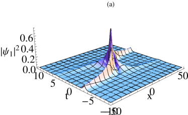
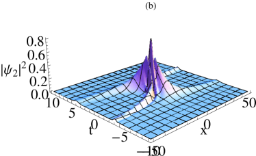
Figure 7: Density profile of two rogue waves for $\eta(t)=2cos(0.15t),g_{2}=0.5,e_{1}=\frac{0.5}{3},\Gamma(t)=0.15t,$ and $f(t)=cos(0.15t)$

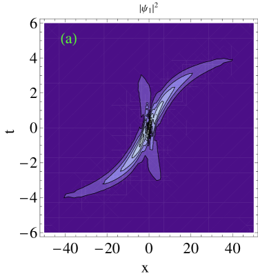
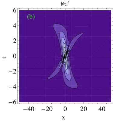
Figure 8: Contour plots of fig (7)

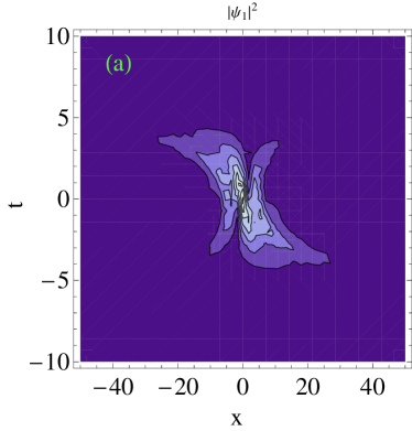
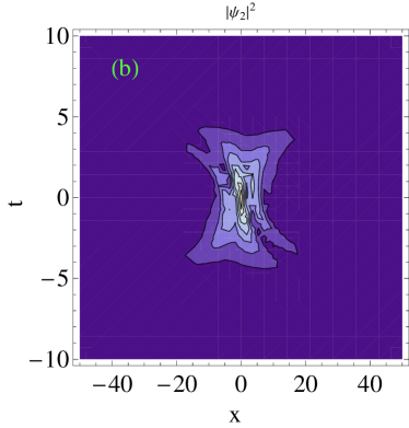
Figure 9: Evolution of two rogue waves with an increased lifespan by finetuning the trapping frequency for $\Gamma(t)=0.1t$

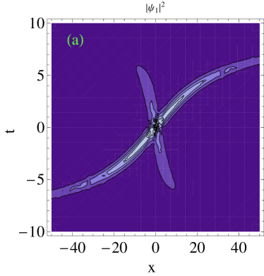
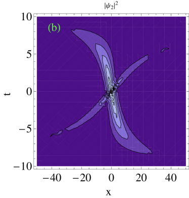
Figure 10: Profile of rogue waves with an increased lifespan by finetuning the trapping frequency for $\Gamma(t)=0.03t$

V Conclusion

In this paper, we discuss the dynamics of the rogue waves of the vector BECs governed by the symmetric coupled GP equation. We observe that we are able to stabilize (or tame) the rogue waves by either manipulating the scattering length (both constant and time dependent) through Feshbach resonance or the trapping frequency. In the process, we end up increasing the lifespan of rogue waves, a new phenomenon which may have wider ramifications in BECs and nonlinear optics.

Acknowledgements:PSV wishes to thank UGC and DAE-NBHM for the financial support. RR wishes to acknowledge the financial assistance received from DAE-NBHM (Ref.No:2/ 48(1)/ 2010 / NBHM /-R and D II/ 4524 dated May.11.2010), UGC (Ref.No:F.No 40-420/2011(SR) dated 4.July.2011) and DST (Ref.No:SR/S2/HEP-26/2012). KP acknowledges DST and CSIR, Government of India, for the financial support through major projects. Authors thank the anonymous referees for their suggestions to improve the readability of the paper.

References

• (1) Z. Y. Yan, Phys. Lett. A 374, 672 (2010).
• (2) R. Smith, J. Fluid Mech. 77, 417 (1976).
R. G. Dean, in Water Wave Kinetics, Ed. by A. Torum and O. T. Gudmestad (Kluwer Academic, Dordrecht, 1990), p. 609.
I. V. Lavrenov, Nat. Hazards 17, 117 (1998).
• (3) E. Pelinovsky and C. Kharif, Extreme Ocean Waves (Springer, Berlin, 2008).
• (4) N. Akhmediev, A. Ankiewicz, and M. Taki, Phys. Lett. A 373 675 (2009).
• (5) D. H. Peregrine, J. Aust. Math. Soc. Ser. B, Appl. Math. 25 16 (1983).
• (6) T. B. Benjamin and J. E. Feir, J. Fluid Mech. 27 417 (1967).
• (7) V. I. Bespalov and V. I. Talanov, Zh. Eksp. Teor. Fiz. Pisma Red. 3, 471 (1966) (JETP Lett. 3, 307 (1966)).
• (8) D. R. Solli, C. Ropers, P. Koonath, and B. Jalali, Nature (London) 450 1054 (2007).
M. Erkintalo, G. Genty, and J. M. Dudley, Opt. Lett. 34, 2468 (2009).
• (9) W. M. Moslem, P. K. Shukla, and B. Eliasson, Europhys. Lett. 96 25002 (2011).
• (10) Y.V. Bludov, V.V. Konotop, and N. Akhmediev, Phys. Rev. A 80 033610 (2009).
• (11) Jingsong He, H.R.Zhang,L.H.Wang, K.Porsezian and A.S.Fokas, Phys.Rev.E 87 0053202 (2013); Boling Guo, Liming Ling and Q.P.Liu, Phys.Rev.E. 85 026607 (2012)
• (12) N. Akhmediev, J.M. Soto-Crespo, and A. Ankiewicz, Phys. Rev. A 80 043818 (2009)
• (13) Zhenya Yana, Dongmei Jiang, Journal of Mathematical Analysis and Applications 395 542 (2012)
• (14) GUO Bo-Ling, LING Li-Ming, Chin. Phys. Lett. 28 110202 (2011)
• (15) Zhenyun Qin, Gui Mu, Phys. Rev. E 86 036601 (2012)
• (16) M. Onorato, A.R. Osborne, M. Serio, Phys. Rev. Lett. 96 014503 (2006)
• (17) P.K. Shukla, I. Kourakis, B. Eliasson, M. Marklund, L. Stenflo, Phys. Rev. Lett. 97 094501 (2006)
• (18) Yu.V. Bludov, V.V. Konotop, N. Akhmediev, Eur. Phys. J. Special Topics 185 169 (2010)
• (19) Yu.V. Bludov, R.Driben, V.V.Konotop and B.A.Malomed, J.Optics. 15 064010 (2013)
• (20) Lin Wen, L.Li, Z.D.Li, S.W. Song, X.F. Zhang and W.M. Liu, Eur.Phys.J.D. 64 473 (2011)
• (21) M. R. Matthews, B. P. Anderson, P. C. Haljan, D. S. Hall, M. J. Holland, J. E. Williams, C. E. Wieman, and E. A. Cornell., Phys. Rev. Lett 83 3358 (1999)
• (22) C.J. Pethick, H. Smith, Bose Einstein Condensation in Dilute Gases, Cambridge Univ. Press, Cambridge, 2003 ; L. Pitaeveskii and Stringari, Bose Einstein Condensation (Oxford University Press, 2003)
• (23) S. Rajendran, P. Muruganandam, M. Lakshmanan. J. Phys. B: At. Mol. Opt. Phys. 42 145307 (2009)
• (24) V. Ramesh Kumar, R. Radha and M.Wadati, Phys. Lett. A 374 3685 (2010)
• (25) L.-L. Chau, J.C. Shaw, H.C. Yen, J. Math. Phys.32 1737(1991)