A Path-Based Distance for Street Map Comparison

Abstract

Comparing two geometric graphs embedded in space is important in the field of transportation network analysis. Given street maps of the same city collected from different sources, researchers often need to know how and where they differ. However, the majority of current graph comparison algorithms are based on structural properties of graphs, such as their degree distribution or their local connectivity properties, and do not consider their spatial embedding. This ignores a key property of road networks since the similarity of travel over two road networks is intimately tied to the specific spatial embedding. Likewise, many current algorithms specific to street map comparison either do not provide quality guarantees or focus on spatial embeddings only.

Motivated by road network comparison, we propose a new path-based distance measure between two planar geometric graphs that is based on comparing sets of travel paths generated over the graphs. Surprisingly, we are able to show that using paths of bounded link-length, we can capture global structural and spatial differences between the graphs.

We show how to utilize our distance measure as a local signature in order to identify and visualize portions of high similarity in the maps. And finally, we give an experimental evaluation of our distance measure and its local signature on street map data from Berlin, Germany and Athens, Greece.

Mahmuda Ahmed, Brittany Terese Fasy, Kyle Hickmann, and Carola Wenk. A Path-Based Distance for Street Map Comparison.

This work is supported by the National Science Foundation, under grant CCF-1301911.

Author’s addresses: M. Ahmed, Computer Science Department, University of Texas at San Antonio; B. T. Fasy and C. Wenk, Computer Science Department, Tulane University; K. Hickmann, Center for Computational Science, Tulane University

1 Introduction

Comparing two embedded graphs is important in the field of transportation network analysis. Often, there exist more than one record of a given transportation network; for example, multiple records can exist when a road network is reconstructed from data. In this case, we would want a method to evaluate the accuracy of the reconstruction against the true map. Moreover, the ability to compare one road network map with a newer map allows one to quantitatively determine the amount of change the transportation network has experienced. Given the street maps of the same city collected from different sources, the goal of this paper is to understand how and where the road maps differ. Figure 2 shows two sets of street maps for the same region of Berlin, Germany and Athens, Greece; while many features are shared, there are large differences, and the goal is to quantify such differences.

The task of comparing street maps has received attention lately with the emergence of algorithms to reconstruct street maps from GPS trajectory data. The OpenStreetMap project provides street map data open to the public, and recently several automatic street map reconstruction algorithms have been proposed in Aanjaneya:2011:MGR:1998196.1998203, csm_esa2012, Biagioni:2012:MIF:2424321.2424333, cghsRnrop10, DBLP:conf/nips/GeSBW11, Karagiorgou:2012:VTD:2424321.2424334, and Liu:2012:MLS:2339530.2339637. However, evaluating the quality of the reconstructed networks remains a challenge. From a theoretical point of view, the problem is deceivingly simple to state:

Given two embedded planar graphs, how similar are they?

Stated this way, there seems to be an immediate connection to the NP-hard subgraph isomorphism problem,which requires a one-to-one mapping between edges and vertices of two graphs. Given two graphs $G$ and $H$, it is NP-hard to determine if there exists a sub-graph of $G$ which is isomorphic to $H$. There has been much work on the subgraph isomorphism problem, and for very restricted classes of graphs it has been shown to be solvable in polynomial time [Eppstein (1995)]. The desired mapping for street map comparison, however, is not necessarily one-to-one and requires spatial proximity; specifically, we desire a distance measure between two networks that indicates when it feels the same to travel over the two networks. That is, navigation on the two transportation graphs works similarly.

Since we are assuming that the two networks being compared are embedded in the plane, it is tempting to just treat the networks as sets of points and use something well-known like the Hausdorff distance to evaluate similarity. However, one could then allow networks with disconnected travel paths to be very similar, even though driving routes on the two would necessarily be very different. We are not aware of any algorithms with theoretical quality guarantees that explicitly require travel paths on the two networks to be similar for the networks themselves to be considered similar.

A second method of studying graph comparison is the graph edit distance. This measure defines similarity between $G$ and $H$, by quantifying how much $H$ must be changed so that it is isomorphic to $G$. DBLP:conf/wea/CheongGKSS09 defined geometric graph distance inspired by the graph edit distance, applied to Chinese character recognition. But, unlike graph edit distance they restricted the operations to follow a specific sequence: 1. edge deletions, 2. vertex deletions, 3. vertex translations, 4. vertex insertions, and 5. edge insertions. The authors showed that their distance measure is NP-hard to compute, and they introduced a new landmark distance that uses vertex distance signatures around landmarks and employs the earth mover’s distance. The geometric graphs in their context, however, are embedded in two different coordinate systems.

Graph comparison lies at the core of many applied and theoretical research avenues, and has been studied by both theoretical and applied communities, see cfsvTYGM04 for a review. But often, additional domain-specific information is used. For example, while Chinese characters consist of graphs, the state-of-the-art in Chinese character recognition relies on additional knowledge, such as the hierarchical structure of the characters or the individual strokes, and, sometimes, the stroke sequence [A. and Madhvanath (2014), Shi et al. (2003), Kim et al. (1996)]. In the context of street map comparison, MondzechS11 and Karagiorgou:2012:VTD:2424321.2424334 have used shortest paths, independently computed in each graph between randomly selected locations, to compare graphs. Liu:2012:MLS:2339530.2339637 and Biagioni:2012:MIF:2424321.2424333 have used bottleneck matching to compare point sets induced by the two graphs. Another recent approach uses a technique from computational topology to compare local graph structures [Ahmed et al. (2014a)]. These approaches, however, do not provide precise guarantees on how similar navigating over the two networks will be if the distance measures are small.

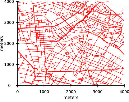
(a) TeleAtlas, Berlin-small.

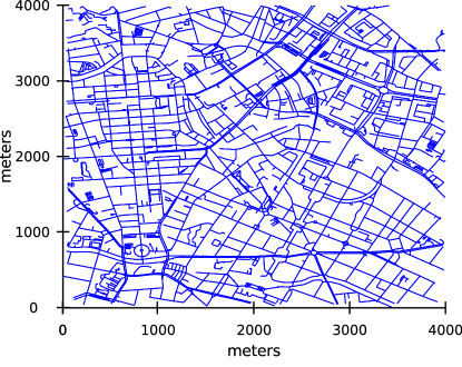
(b) OpenStreetMap, Berlin-small.

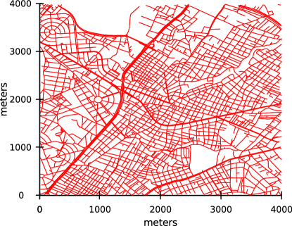
(c) TeleAtlas, Athens-small.

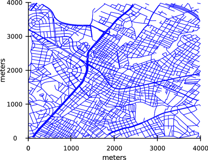
(d) OpenStreetMap, Athens-small.

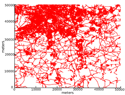
(e) TeleAtlas, Berlin-large.

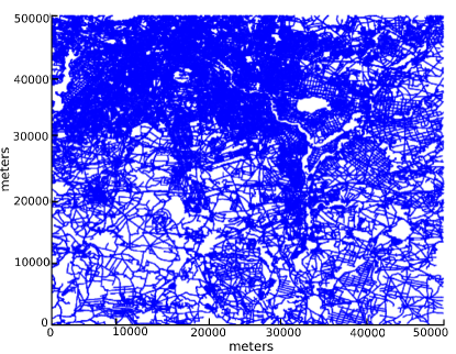
(f) OpenStreetMap, Berlin-large.

Figure 1: The TeleAtlas (TA) and OpenStreetMap (OSM) maps for the same square sections of Berlin and Athens. For both Berlin datasets, OSM has more detail than TA and for Athens-small, TA has more detail than OSM. Among these datasets, Athens-small maps are the most similar to each other.

In judging the difference between two street maps, intuitively, one is concerned with the utility of the street map graphs as a navigation tool. Therefore, we propose a distance measure on street map graphs based on similarities of the possible travel routes allowed by the networks. Here, a street map is formally defined as a planar geometric graph $G$, with vertices $V_{G}\subseteq\mathbb{R}^{2}$ and edges $E_{G}$ given by polygonal paths embedded in ${\mathbb{R}}^{2}$ connecting two different vertices in $V_{G}$. In this framework, it is possible to have more than one edge connecting two vertices. Under this definition the graph $G$ can be treated as a set of possible paths in $\mathbb{R}^{2}$, as opposed to treating the graph as a set of points in $\mathbb{R}^{2}$. Since paths of travel are implicitly considered with our measure, closeness in this distance represents similarity of navigation.

Our Contributions

We introduce a new distance measure for planar embedded geometric graphs $G$ and $H$, which is based on covering $G$ and $H$ with sets of paths. The distance measure is the directed Hausdorff distance between the path sets, where the Fréchet distance is used to compute the distance between two paths. We have emphasized use of the directed Hausdorff distance, since often in the map reconstruction problem, the reconstruction only represents a subgraph of the larger transportation network. Thus, we are interested in measuring the second graph’s closeness to an appropriate subgraph of the true transport network.

In Section 3, we provide the theoretical guarantees of the path-based distance. Restricting our attention to paths with small link-length, we are able to capture the structural as well as the spatial properties of the graphs. Using link-length one paths, we compute a generalization of the Hausdorff distance. Using link-length two paths, we capture intersections. Most surprisingly, using only link-length three paths, we are able to approximate the distance between paths of arbitrary link-length in polynomial time.

In Subsection 3.4, we show how to utilize our distance measure as a local signature in order to identify and visualize portions of high similarity, or of dissimilarity, between the maps. Such local information is useful for detecting changing areas in road networks using historical map comparison and for identifying types of street map formations that reconstruction algorithms may fail at detecting. Finally, in Section 4, we give an experimental evaluation of our distance measure and its local signature on street map data from Berlin, Germany and Athens, Greece. The code for computing our path-based distance is available on mapconstruction.org.

2 Street Map Graphs

We model a street map as a planar geometric graph, $G=(V_{G},E_{G})$, embedded in $\mathbb{R}^{2}$. We assume that each edge in $E_{G}$ is represented as a polygonal curve and that no vertex in $V$ has degree two. That is, intersections in the street maps become vertices and roadway segments with no intersections make up the edges.

2.1 Comparing Street Maps

When designing a distance measure to compare two street map graphs, we would like to incorporate the following features:

1. Spatial distance between corresponding vertices of the two graphs.

2. Similarity of the shapes of the edges.

3. Similar connectivity properties, i.e., similar navigation.

Difficulties can arise in evaluating whether or not the above three criteria have been accounted for properly. For example, split and merge vertices (see Figure 2) may arise from different street map construction mechanisms. In both subfigures, one can find a path on the blue graph that is close to any arbitrary path on the dashed pink graphs. Moreover, for every vertex on the pink graphs there is a close vertex on the blue graph. While designing the measure we wanted to make sure sure not to penalize too much for such cases but yet find these differences. In general, the current approaches to street map comparison fall into two categories. The first one treats the graph as a set of points in the plane the second one treats the graph as a set of paths. Here, we briefly discuss the ideas.

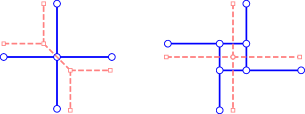
Figure 2: Two graphs $G$ (solid blue lines) and $H$ (dashed pink lines). (a) One vertex in $G$ represented as two vertices in $H$. (b) Four vertices in $G$ represented as one vertex in $H$.

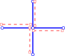
(a) Four components.

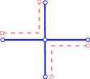
(b) Missing vertex.

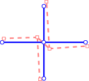
(c) Split vertex.

Figure 3: (a), (b), (c): Two graphs $G$ (solid blue lines) and $H$ (dashed pink lines). The path-based distance using $\Pi^{1}_{G}$ is small despite large differences in combinatorial structures.

Sets of Points

This approach treats each graph as the set of the points that its vertices and edges cover in the plane. The main idea is then to compute a distance measure between two point sets, such as the Hausdorff distance between the infinite complete set of points, or a one-to-one bottleneck matching between a carefully selected finite subset of the points. The main drawback of using regular Hausdorff distance is that no adjacency information is used, and the continuous structure of the graphs is largely ignored. Thus, in Figure 3, the dashed pink graphs in (a), (b), and (c) would all be considered close to the solid blue graph under this distance measure. However, their connectivity properties are all very different and the set of possible travel paths would be quite different.

The measure in Biagioni:2012:MIF:2424321.2424333 compares the geometry and topology of the graphs by sampling its edges. The main idea is as follows: starting from a random street location $p$ (the seed), walk in both directions, choosing a sample point at regular intervals. If an intersection is encountered, continue along every path possible until a maximum distance from the seed is reached. Repeating for the other graph using the closest point to $p$ as the seed, two sets of locations are obtained. These two point sets are compared by finding a maximal bottleneck matching between them and counting the number of unmatched points in each set. The sampling process is repeated for several seed locations, and a global tally of the matched and unmatched samples in each graph is recorded. In essence, the local neighborhoods of the seeds have been sampled, and these samples are compared in the matching. For the bottleneck matching, the sample points on one graph can be considered as marbles and on the other graph as holes. Intuitively, if a marble lands close to a hole it falls in, marbles that are too far from a hole remain where they land, and holes with no marbles nearby remain empty. Each hole, however, can hold at most one marble. Then the number of matched marbles (equal to the number of matched holes) is counted.

To produce a performance measure, Biagioni:2012:MIF:2424321.2424333 use the well-known $F$-score, which they compute as follows:

$$F\text{-score}=2*\frac{precision*recall}{precision+recall}$$ (1)

where, $precision$ is defined to be $matched\_marbles/total\_marbles$ and $recall$ is defined to be $matched\_holes/total\_holes$. In words, the precision measures the percentage of the marbles that are matched to holes and the recall measures the percentage of the holes that are matched to marbles. The $F$-score can range between zero and one, with a score close to one indicating that nearly all holes and marbles are matched, and a score close to zero indicating that very few marbles and holes are matched. In Subsection 4.5, we provide a comparison of our distance measures to this distance measure.

Sets of Paths

The basic idea of this approach is to construct sets of paths to represent the two graphs, and then define a distance measure based on distances between the paths. Different distance measures can be used to compare paths, such as the Hausdorff distance or the Fréchet distance. Referring again to Figure 3, we see that, in (a) and (b), there exist pairs of connected vertices in the blue graph whose corresponding vertices are not connected in the pink dashed graph resulting in a large path-based distance. However, the dashed pink graph in (c) does have a close path connecting the top and bottom vertices so it would be closer in this distance measure. In this way using sets of paths to define a distance measure preserves connectivity properties of the graph. The main challenge in defining a path-based distance measure is then to select a set of paths from one graph such that the set as a whole preserves some structural properties of the graph that can be utilized in an application. Such a set of paths must be small enough to check each path computationally. MondzechS11 have introduced a heuristic measure by comparing shortest path lengths between pairs of randomly selected points. Karagiorgou:2012:VTD:2424321.2424334 have used a similar set of paths, but used the discrete Fréchet distance to compare routes. In this paper we use a more general set of paths.

2.2 Paths

In this paper, we use a path-based approach to compare two embedded geometric graphs. Let $a$ and $b$ be two points on any edge or vertex of $G$. A path in $G$ between $a$ and $b$ is a, possibly non-simple, sequence of vertices in $G$ connecting $a$ to $b$ using valid adjacencies in the graph. We consider such a path to be the image of a continuous map $\alpha\colon[0,1]\to G$ such that $\alpha(0)=a$ and $\alpha(1)=b$. If a path starts and ends in vertices $u,v\in V_{G}$ we call it a vertex-path, and we define its link-length as the number of edges that comprise the path, and we may represent the path as sequence of vertices: $\alpha=\langle uw_{1}w_{2}\cdots w_{k-1}v\rangle$ . Here we remind the reader that the vertices of our graph do not have degree two. This distinction is made since with street maps in mind, we consider only the actual street intersections as graph vertices. We denote the set of all paths in $G$ by $\Pi_{G}$. We denote the set of all vertex-paths of link-length $k$ in $G$ as $\Pi^{k}_{G}$. Let $\hat{\Pi}_{G}=\cup_{k\geq 1}\Pi^{k}_{G}$ be the set of all vertex-paths, then we have that $\hat{\Pi}_{G}\varsubsetneq\Pi_{G}$. Sometimes we may restrict our attention to all paths of link-length $k$ containing vertex $v\in V_{G}$ or an edge $e\in E_{G}$; we denote these restricted sets of paths by $\Pi_{v}^{k}$ and $\Pi_{e}^{k}$, respectively. We denote the Euclidean norm by $\|.\|$. Our distance measure between two embedded graphs are based on the Fréchet distance between two paths.

Definition 2.1 (Fréchet Distance).

For two planar curves $f,g:[0,1]\rightarrow\mathbb{R}^{2}$, the Fréchet distance $\delta_{F}$ between them is defined as

$$\delta_{F}(f,g)=\inf_{\begin{subarray}{c}\alpha:[0,1]\rightarrow[0,1]\end{subarray}}\max_{\begin{subarray}{c}t\in\left[0,1\right]\end{subarray}}\|f(t)-g(\alpha(t))\|,$$ (2)

where $\alpha$ ranges over all continuous, surjective, non-decreasing reparameterizations.

The Fréchet distance is a well-suited distance measure for comparing curves, or paths, because it takes continuity and monotonicity of the curves into account. The Fréchet distance between two polygonal curves with $m$ and $n$ vertices, respectively, can be computed in $O(mn\log mn)$ time [Alt and Godau (1995)]. Furthermore, the Fréchet distance induces a correspondence between the curves:

Corollary 2.2 (Induced Correspondence).

Let $\delta=\delta_{F}(f,g)$. Then, there exists a continuous function $C\colon[0,1]\to[0,1]^{2}$ such that $C$ is non-decreasing in each coordinate and $||f(s)-g(t)||\leq\delta$ for all $(s,t)$ in the image of $C$. We define the function $M\colon\mathrm{im}{f}\to\mathrm{im}{g}$ where $f(s)\mapsto g(\min\{t|(s,t)\in\mathrm{im}{C}\})$. And we define the generalized inverse $M^{-1}\colon\mathrm{im}{g}\to\mathrm{im}{f}$ where $g(t)\mapsto f(\min\{s|(s,t)\in\mathrm{im}{C}\})$.

In words, $C$ provides a parameterization that realizes the Fréchet distance between the curves. We refer to $M$ as the Fréchet-correspondence from $f$ to $g$. Also, we note that $C$ (and hence $M$) need not be unique; however, it will suffice to choose an arbitrary correspondence $C$. We extend $M$ to a function $\overline{M}$ from sub-paths of $f$ to sub-paths of $g$ as follows: $\overline{M}(p)$ is the shortest connected sub-path of $g$ containing all points $M(x)$, where $x\in p$ and $p$ is a sub-path of $f$.

In the map-matching problem, we ask to find a path $h\in H$ that minimizes the distance to a given curve $g\in G$. In our setting, we wish to minimize the Fréchet distance $\delta_{F}(g,h)$. We call this map-matching the Fréchet-matching and denote it by $\delta_{F}(g,H)$. This distance can be computed in $O(mn\log^{2}mn)$ time [Alt et al. (2003)], where $m$ is the number of vertices in $g$ and $n$ is the total number of vertices and edges in $H$. The directed distance that we define in the next section is the maximum map-matching distance over all paths $g\in G$.

3 Path-Based Distance

In this section, we formally define a path-based distance between street map graphs. The general idea is to summarize each graph with a set of paths, and then to compare these sets using the directed Hausdorff distance. The directed Hausdorff distance between two sets $A$ and $B$ is defined as $\overrightarrow{d}(A,B)=\max_{a\in A}\min_{b\in B}d(a,b)$. Usually, $d(a,b)$ is assumed to be the Euclidean distance. However, the sets we are considering are the sets of all paths on two different road network maps. Therefore we require a distance between two paths instead of the standard Euclidean distance. For this, we use the Fréchet distance between paths.

Definition 3.1 (Path-Based Distance).

Let $G$ and $H$ be two planar geometric graphs, and let $\pi_{G}\subseteq\Pi_{G}$ and $\pi_{H}\subseteq\Pi_{H}$. The directed path-based distance between these path sets is defined as:

$$\overrightarrow{d}_{path}(\pi_{G},\pi_{H})=\max_{p_{G}\in\pi_{G}}\min_{p_{H}\in\pi_{H}}\delta_{F}(p_{G},p_{H}).$$ (3)

The undirected version of the distance, $d_{path}(\pi_{G},\pi_{H})$ is defined to be the maximum of the two directional distances $\overrightarrow{d}_{path}(\pi_{G},\pi_{H})$ and $\overrightarrow{d}_{path}(\pi_{H},\pi_{G})$, similar to the undirected Hausdorff distance. Like the Hausdorff distance, the path-based distance is not symmetric, i.e., $\overrightarrow{d}_{path}(\pi_{G},\pi_{H})\neq\overrightarrow{d}_{path}(\pi_{H},\pi_{G})$. This anti-symmetry is desirable in our setting. For example, $G$ could be the reconstructed road network from bus route data. In this case, the bus routes only correspond to a subgraph of the complete road network so the directed distance is more informative.

The question now is how to define path sets $\pi_{G}$ and $\pi_{H}$ that yield a suitable distance measure between $G$ and $H$. Recall from above that $\Pi_{G}$ is the set of all paths in $G$, and $\widehat{\Pi}_{G}$ is the set of all paths in $G$ that start and end in a vertex. Ideally, $\pi_{G}=\Pi_{G}$ and $\pi_{H}=\Pi_{H}$, in order to capture the most structure from both graphs. Interestingly, whether paths in $G$ start and end in a vertex or anywhere on an edge, does not affect the path-based distance.

Lemma 3.2 (Vertex-Paths).

Let $G,H$ be two graphs. Then, the following equality holds: $\overrightarrow{d}_{path}(\Pi_{G},\Pi_{H})=\overrightarrow{d}_{path}(\widehat{\Pi}_{G},\Pi_{H})$.

Proof 3.3.

For every $p\in\Pi_{G}$, there exists a path $\widehat{p}\in\widehat{\Pi}_{G}$ such that $p$ is a sub-path of $\widehat{p}$, we have that $\overrightarrow{d}_{path}(\Pi_{G},\Pi_{H})\leq\overrightarrow{d}_{path}(\widehat{\Pi}_{G},\Pi_{H})$. In addition, from the inclusion $\widehat{\Pi}_{G}\varsubsetneq\Pi_{G}$ follows $\overrightarrow{d}_{path}(\widehat{\Pi}_{G},\Pi_{H})\leq\overrightarrow{d}_{path}(\Pi_{G},\Pi_{H})$.

But still, these complete path sets are infinite in size, so an exhaustive comparison is out of the question. Fortunately, if we restrict ourselves to a polynomial number of paths in $\pi_{G}$, while $\pi_{H}=\Pi_{H}$, then $\overrightarrow{d}_{path}(\pi_{G},\Pi_{H})=\max_{p_{G}\in\pi_{G}}\delta_{F}(p_{G},H)$ can be computed in polynomial time, by computing a polynomial number of map-matching distances [Alt et al. (2003)].

In what follows, we analyze the path-based distance for different subsets of paths $\pi_{G}\subset\Pi_{G}$ and fix $\pi_{H}=\Pi_{H}$. In particular, we will closely examine what properties of the graphs $G$ and $H$ must be similar for $\overrightarrow{d}_{path}(\cdot,\cdot)$ to be small when considering only paths of fixed link-length in $G$. For brevity, we define the following notation for path-based distances for commonly used path sets.

Definition 3.4 (Path-Based Distance for Common Path Sets).

The overall path-based distance for graphs $G$ and $H$ is defined as $\Delta:=\overrightarrow{d}_{path}(\Pi_{G},\Pi_{H})$. Let $v\in V_{G}$ be a vertex, $e\in E_{G}$ be an edge, and let $k\geq 1$ be an integer. We define $\Delta_{v}:=\overrightarrow{d}_{path}(\Pi_{v},\Pi_{H}),\Delta_{e}:=\overrightarrow{d}_{path}(\Pi_{e},\Pi_{H})$, and $\Delta_{k}:=\overrightarrow{d}_{path}(\Pi_{G}^{k},\Pi_{H})$. And we define $\Delta_{k,v}:=\overrightarrow{d}_{path}(\Pi_{v}^{k},\Pi_{H})$ and $\Delta_{k,e}:=\overrightarrow{d}_{path}(\Pi_{e}^{k},\Pi_{H})$.

If two end vertices of an edge $e\in E_{G}$ are $v_{1}$ and $v_{2}$ then $\Delta_{k,e}\leq\min\left(\Delta_{k,v_{1}},\Delta_{k,v_{2}}\right)$ as $\Pi_{e}^{k}\subseteq\Pi_{{v_{1}}}^{k}\cap\Pi_{{v_{2}}}^{k}$. Observe that each path of link-length two $\langle uvw\rangle$ can be extended to a path of link-length three by adding the second edge backward $\langle uvwv\rangle$. Extending this observation, we obtain the following:

Lemma 3.5 (Monotonicity).

$\Delta_{k}$, $\Delta_{k,v}$ and $\Delta_{k,e}$ are non-decreasing in $k$.

Proof 3.6.

Let $p\in\Pi_{G}^{k}$. We can then write $p=\langle v_{1},v_{2},\ldots,v_{k-1},v_{k}\rangle$ for some set of vertices $v_{1},\ldots,v_{k}\in G$. Then, $p^{\prime}=\langle v_{1},v_{2},\ldots,v_{k-1},v_{k},v_{k-1}\rangle$ is a vertex-path in $\Pi_{G}^{k+1}$. Since $\overrightarrow{d}_{path}(\{p\},\Pi_{H})=\overrightarrow{d}_{path}(\{p^{\prime}\},\Pi_{H})$ and $\{p^{\prime}|p\in\Pi_{G}^{k}\}\subseteq\Pi_{G}^{k+1}$, we can conclude that $\Delta_{k}$ is non-decreasing in $k$. The proof is analogous for $p\in\Pi_{v}^{k}$ or $p\in\Pi_{e}^{k}$.

Hence, it will be sufficient to compute $\lim_{k\to\infty}\overrightarrow{d}_{path}(\Pi^{k}_{G},\Pi_{H})$ in order to compute the path-based distance between street map graphs $G$ and $H$. Here, we write $k\to\infty$ even though, for a finite graph there is a maximum possible size for $k$ which, however, is computationally infeasible to use.

3.1 Paths of Link-Length One

First, we consider the case where $\pi_{H}=\Pi_{H}$ is the set of all paths in $H$ and $\pi_{G}=\Pi^{1}_{G}=E_{G}$ consists of all paths of link-length one. In this case, one can only ensure that for each edge $e\in E_{G}$ there is a similar path $p_{H}$ in $H$ such that $\delta_{F}(e,p_{H})\leq\overrightarrow{d}_{path}(\Pi^{1}_{G},\Pi_{H})$. As $\Pi^{1}_{G}$ does not model the existence of a vertex incident to two edges, a small $\overrightarrow{d}_{path}(\Pi^{1}_{G},\Pi_{H})$ does not guarantee connections between edges of $H$. In this case, different choices of $H$ with very different combinatorial structure can have the same distance from $G$, as shown in Figure 3. Thus, the similarity of travel-paths is not captured using only link-length one paths.

3.2 Paths of Link-Length Two

Next, we consider the case where $\pi_{H}=\Pi_{H}$ and $\pi_{G}=\Pi^{2}_{G}$ consists of all paths of link-length two. For this case, we can define a correspondence between $V_{G}$ and $V_{H}$ under reasonable assumptions on $G$ that guarantee the vertices of $G$ are sufficiently spread out from each other and are at least of degree four. The key observation here is that $\Pi^{2}_{{v}}$ preserves all adjacency transitions around a vertex $v$, because by definition $\langle v_{i}vv_{j}\rangle\in\Pi^{2}_{{v}}$ for all $v_{i},v,v_{j}\in V_{G}$ with $v_{i},v_{j}\in\mbox{Adj}(v)$. Here, we used $\mbox{Adj}(v)\subseteq V$ to denote the set of vertices adjacent to $v\in V$.

Letting $e_{i}$ be the edge $vv_{i}$, we define:

Definition 3.7 (Intersection Radius).

Given edges $e_{0},e_{1},e_{2},\ldots,e_{n}$ with common endpoint $v$, we will define the intersection radius at scale $d$, denoted by $r_{d}(v)$. Let $B$ be a ball of radius $r$ centered at $v$. We can then choose a point $w_{i}\in e_{i}\cap\partial B$ uniquely, if it exists, by starting at $v$ and walking along $e_{i}$ until we reach $\partial B$. Let $r_{d}(v)$ denote the minimum radius such that $w_{i}$ exists for all $e_{i}$ and $||w_{i}-w_{j}||>2d$ for all $i\neq j$. If such a radius does not exist, then $r_{d}(v)=\infty$. We call $r_{d}(v)$ the intersection radius at $v$, and we define $r_{d}=\max_{v\in V}r_{d}(v)$.

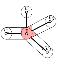
(a) Intersection region.

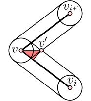
(b) Computing $||v-v^{\prime}||$.

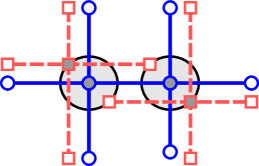
(c) Vertex correspondence.

Figure 4: (a) By definition, $\Pi^{2}_{G}$ contains all paths of link-length two. If a vertex has at least four neighbors, then we can find a transverse intersection: $v_{2}vv_{4}$ and $v_{1}vv_{3}$. (b) The distance $d(v,v^{\prime})=\Delta/\sin(\theta_{v}/2)$ is the hypotenuse of the right triangle shown in pink. (c) Two graphs $G$ and $H$; edges in $G$ are solid blue and edges in $H$ are dashed pink.

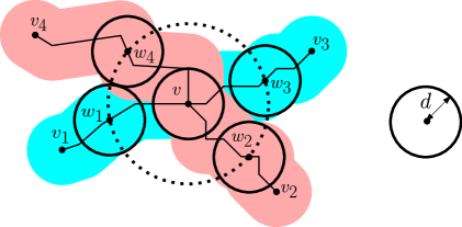
Figure 5: The intersection radius $r_{d}(v)$ is the smallest radius such that each ball of radius $d$ centered at $\{w_{i}\}$ contains only one of the two paths. In this example, $v$ is $d$-separated since such a radius exists.

In the case that the edges are line segments, we denote with $\theta_{v}$ the smallest angle formed by any two distinct edges at $v$, and we call this angle the minimum angle at vertex $v$. In this case, the computation of $r_{d}(v)$ is straightforward:

Lemma 3.8 (Straight Edge Intersection Radius).

If all of the edges incident to $v$ are line segments and if $r_{d}(v)$ is defined, then $r_{d}(v)=d/\sin(\theta_{v}/2)$.

The distance $\Delta_{k,v}/\sin{(\theta_{v}/2)}$ is found by computing the hypotenuse of the pink triangle in Figure 4(b).

The theoretical guarantees that we give below work for well-separated vertices that have sufficiently high degree. In particular, we are interested in the cases where $d=\Delta$, $\Delta_{v}$, or $\Delta_{k,v}$ as defined at the end of the introduction to this section. In this way, the specific amount of vertex separation we require is dependent upon which subset of paths our distance measure is being evaluated; see Figure 5.

Definition 3.9 ($d$-separated Vertex).

A vertex $v\in G$ is $d$-separated if $r_{d}(v)$ is finite.

Having $d$-separated vertices of degree at least four implies that vertex-paths crossing in $G$ will have corresponding crossing paths in $H$:

Theorem 3.10 (Crossing Paths).

Let $p_{1}$, $p_{2}$ be two vertex-paths in $G$ that intersect transversely at a $d$-separated vertex $v$. If $p_{1}^{\prime},p_{2}^{\prime}$ are two paths in $H$ with $\delta_{F}(p_{1},p_{1}^{\prime}),\delta_{F}(p_{2},p_{2}^{\prime})<d$, then $p_{1}^{\prime}$ and $p_{2}^{\prime}$ must intersect.

Proof 3.11.

Let $w_{1}$,$w_{3}$ (similarly, $w_{2}$,$w_{4}$) be the first intersections of $p_{1}$ ($p_{2}$) with the ball $B$ of radius $r_{d}(v)$ centered at $v$, as shown in Figure 5. The path connecting $w_{1}$ and $w_{3}$ has a corresponding path $\tilde{p}_{1}$ in $H$ within Fréchet distance $d$. Notice that this path necessarily divides $B$ into two sets: one containing $w_{2}$ and one containing $w_{4}$. Therefore, the path $\tilde{p}_{2}$ in $H$ with Fréchet distance at most $d$ from the path connecting $w_{2}$ and $w_{4}$ must intersect $\tilde{p}_{1}$.

The previous theorem implies the following corollary that path-correspondences between link-length two paths in $G$ to paths in $H$ imply a guaranteed vertex correspondence between vertices in $G$ to vertices in $H$.

Corollary 3.12 (Vertex Correspondence).

If a vertex $v\in G$ has degree at least four and is $\Delta_{k,v}$-separated for some $k\geq 2$, then there exists a corresponding vertex $v^{\prime}$ in $H$ such that $||v-v^{\prime}||\leq r_{d}(v)+d$.

Considering the example given in  Figure 4(a), two paths that cross transversely at $v$ in $G$ will have a corresponding vertex $v^{\prime}$ in $H$ somewhere in the pink region containing $v$.

3.3 Paths of Link-Length $k$ for $k\geq 3$

As we have seen in the last section, the path-based distance formed using the set $\Pi^{2}_{G}$ of paths of link-length two allows us to define a particular vertex correspondence between $G$ and $H$ at vertices of the road network that are not too tightly clustered. However, the distance $\overrightarrow{d}_{path}(\Pi^{2}_{G},\Pi_{H})$ can still be small for a connected graph $G$ and a graph $H$ with multiple connected components, as is the case in Figure 4(c). In this section, we analyze what additional guarantees can be provided by considering $\Pi^{k}_{G}$ for $k\geq 3$.

We prove that $\overrightarrow{d}_{path}(\Pi_{G},\Pi_{H})$ can be approximated by $\overrightarrow{d}_{path}(\Pi^{3}_{G},\Pi_{H})$ as long as assumptions about how much vertices in $G$ are clustered are met. This is accomplished by showing that if all link-length three paths in $G$ have a close path in $H$, then for any path in $G$, there is a close path in $H$ as well. This yields a polynomial-time algorithm to approximate $\overrightarrow{d}_{path}(\Pi_{G},\Pi_{H})$ when all vertices in $G$ are well-separated, overcoming the infinite complexity of using the full set of paths, $\Pi_{G}$, to define our path-based distance.

The following theorem shows that path-correspondences between link-length three paths in $G$ to paths in $H$ suffice to guarantee correspondences for longer paths (of link-length four).

Theorem 3.13 (Link-Length Three Surgeries).

Let $p=v_{0}v_{1}v_{2}v_{3}v_{4}$ be a vertex-path of link-length four in $G$, such that each vertex $v$ in $p$ is $\Delta_{3,v}$-separated and does not have degree three. Then $\delta_{F}(p,H)\leq 2r_{d}(v_{2})+d$, where $d=\Delta_{3,v_{2}}$.

Proof 3.14.

The general idea of this proof is as follows: We will find two paths in $G$, which intersect at $v_{2}$. Then, we will find the corresponding paths in $H$ and stitch them together to find a path close to $p$.

We examine vertex $v_{2}$, which has degree at least four. Let $v_{2}^{a}$ and $v_{2}^{b}$ be two neighbors of $v_{2}$ which are neither $v_{1}$ nor $v_{3}$; see Figure 6 for the two possible configurations. Let $p_{ab}$ be the path $v_{2}^{a}v_{2}v_{2}^{b}$ and $p_{13}$ be the path $v_{1}v_{2}v_{3}$.

(a) Case a: surgery on transverse paths.

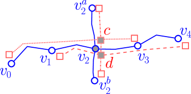
(b) Case b: surgery on parallel paths.

Figure 6: We see two configurations of graphs $G$ (solid blue lines) and $H$ (dashed pink lines). In Theorem 3.13, we show that for each path of link-length $\geq 4$, we can construct a corresponding path in $H$ by performing surgery on link-length three paths. The pink paths shown are at most $\Delta_{3,v}$ from the link-length three paths.

Case a: We first assume that $p_{ab}$ and $p_{13}$ form a non-transverse intersection, as in Figure 6(a). Consider the transverse paths $p_{0b}=v_{0}v_{1}v_{2}v_{2}^{b}$ and $p_{a4}=v_{2}^{a}v_{2}v_{3}v_{4}$. Let $p_{0b}^{\prime}$, $p_{a4}^{\prime}$ be the Fréchet-closest paths in $H$ to $p_{0b}$ and $p_{a4}$, respectively. We observe that $\delta_{F}(p_{0b},p_{0b}^{\prime})$ and $\delta_{F}(p_{a4},p_{a4}^{\prime})$ are at most $d=\Delta_{3,v_{2}}$, since $v_{2}\in p_{0b}\cap p_{a4}$.

Let $M_{a}$ be a Fréchet-correspondence between $p_{a4}$ and $p_{a4}^{\prime}$; likewise, let $M_{b}$ be a Fréchet-correspondence between $p_{0b}$ and $p_{0b}^{\prime}$, as defined in . Then, let $\tilde{v}_{2}^{0b}=M_{b}(v_{2})$ and $\tilde{v}_{2}^{a4}=M_{a}(v_{2})$. We know that $|v_{2}-\tilde{v}_{2}^{*}|\leq\Delta_{3,v_{2}}$ since $M_{a}$ and $M_{b}$ are Fréchet-correspondences.

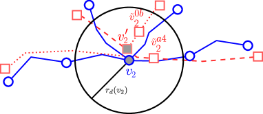
Figure 7: We focus on the intersection region of Figure 6(a). We draw a circle of radius $r_{d}(v_{2})$ centered at $v_{2}$. The path $\rho_{02}^{\prime}$ starts outside the circle and ends at $v_{2}^{\prime}$. It is obtained by shortening the path $p_{02}^{\prime}$, which ends at $\tilde{v}_{2}^{0b}$. The path $\rho_{24}$ is obtained by extending the path $p_{24}$, moving the start vertex from $\tilde{v}_{2}^{a4}$ to $v^{\prime}_{2}$.

Next, we find an intersection of $p_{0b}^{\prime}$ and $p_{a4}^{\prime}$ close to $\tilde{v}_{2}^{0b}$ and $\tilde{v}_{2}^{a4}$. If $\tilde{v}_{2}^{0b}=\tilde{v}_{2}^{a4}$, then we have already found that intersection. Otherwise, assume $\tilde{v}_{2}^{0b}\neq\tilde{v}_{2}^{a4}$, as shown in Figure 7. Let ${\mathbb{B}}$ be the ball of radius $r_{d}(v_{2})$ centered at $v_{2}$. Let $e_{1}$ be the edge $v_{2}v_{1}$, $e_{3}$ the edge $v_{2}v_{3}$, $e_{2}^{a}$ the edge $v_{2}v_{2}^{a}$, and $e_{2}^{b}$ the edge $v_{2}v_{2}^{b}$. Then, we can let $w_{i}$ (respectively, $w_{i}^{j}$) be the first intersection of the edge $e_{i}$ $(e_{i}^{j})$ with $\partial{\mathbb{B}}$, as in Definition 3.7. Furthermore, we can partition $\partial{\mathbb{B}}$ into three sets: $A_{0b}:=$ points within $\Delta_{3,v_{2}}$ of $\{w_{1},w_{2}^{b}\}$, $A_{a4}:=$ points within $\Delta_{3,v_{2}}$ of $\{w_{2}^{a},w_{3}\}$, and the leftover points. In particular, each of the first two sets has exactly two connected components: $A_{0b}=A_{0b}^{1}\sqcup A_{0b}^{2}$ and $A_{a4}=A_{a4}^{1}\sqcup A_{a4}^{2}.$ We can think of $A_{0b}^{1}$ and $A_{0b}^{2}$ as corresponding to $p_{0b}$ entering and leaving ${\mathbb{B}}$; see Figure 8, where $A_{0b}$ is in cyan and $A_{a4}$ is in red.

Figure 8: Since $v_{2}$ is $d$-separated for $d={\Delta_{3,v}}$ , the boundary of the gray disc ${\mathbb{B}}$ can be decomposed into three parts, shown in cyan (region $A_{0b}$), red (region $A_{a4}$), and black (neither).

Consider $p_{0b}^{\prime}\cap{\mathbb{B}}$, which could have multiple connected components. Since $v$ is $d$-separated, there exists a unique subpath of $p_{0b}^{\prime}$ that enters on $A_{0b}^{1}$ and leaves on $A_{0b}^{2}$. We call this subpath $q_{0b}^{\prime}$. Similarly, there exists a unique subpath $q_{a4}^{\prime}$ of $p_{a4}^{\prime}$ that enters ${\mathbb{B}}$ on one of $A_{a4}^{1}$ or $A_{a4}^{2}$ and leaves on the other. Notice that $q_{0b}^{\prime}$ and $q_{a4}^{\prime}$ necessarily intersect at least once by Theorem 3.10. Let $v_{2}^{\prime}$ be one of those intersections. We note that we can uniquely choose an intersection by expanding the subpaths around $\tilde{v}_{2}^{0b}$ and $\tilde{v}_{2}^{a4}$ until an intersection is found. Furthermore, the distance between $v_{2}$ and $v_{2}^{\prime}$ is at most $r_{d}(v_{2})+d$ by

We wish to perform surgery on the paths $p_{0b}^{\prime}$ and $p_{a4}^{\prime}$ in order to upper bound the Fréchet distance between $p$ and $H$. Let $p^{\prime}_{02}=\overline{M}_{b}(p_{02})$ and $p^{\prime}_{24}=\overline{M}_{a}(p_{24})$; notice that both $\delta_{F}(p_{02},p^{\prime}_{02})$ and $\delta_{F}(p_{24},p^{\prime}_{24})$ are at most $\Delta_{3,v_{2}}$.

Next, we find a path $\rho_{02}^{\prime}$ in $H$ Fréchet-close to $p_{02}\subset p_{0b}$ that begins at $v_{0}^{\prime}$ and ends at $v_{2}^{\prime}$. In fact, we almost have that path already. Informally, the path that starts with $p^{\prime}_{02}$ and is either extended or shortened so that $v_{2}^{\prime}$ is an endpoint. We elaborate on the two scenarios (extending and shortening):

1. First, suppose we need to extend $p_{02}^{\prime}$, as is the case when $v_{2}^{\prime}$ is not on the path $p_{02}^{\prime}$; see Figure 7. Here, we observe that $d_{F}(p_{0b},p_{0b}^{\prime})\leq d$ and $d_{F}(p_{02},\rho_{02}^{\prime})\leq r_{d}(v_{2})+d$.

2. Second, suppose we need to shorten $p_{02}^{\prime}$. Let $u=M_{b}^{-1}(v_{2}^{\prime})$. Observe $|v_{2}^{\prime}-u|\leq d$ and $|v_{2}^{\prime}-v_{2}|\leq r_{d}(v_{2})+d$, and for any $x$ on the path between $v_{2}$ and $u$, we have $|v_{2}^{\prime}-x|\leq 2r_{d}(v_{2})+d$.

Thus, we have proven that

$$\delta_{F}(p_{02},\rho^{\prime}_{02})\leq 2r_{d}(v_{2})+d$$

Using a similar argument, we can also obtain:

$$\delta_{F}(p_{24},\rho^{\prime}_{24})\leq 2r_{d}(v_{2})+d$$

Hence, concatenating these two subpaths yields the path $p^{\prime}$, which has Fréchet distance at most $2r_{d}(v_{2})+d$ to $p$.

Case b: We now assume that $p_{ab}$ and $p_{13}$ form a transverse intersection, as illustrated in Figure 6(b). We observe that the path $p$ consists of two paths $p_{03}=v_{0}v_{1}v_{2}v_{3}$ and $p_{14}=v_{1}v_{2}v_{3}v_{4}$ of link-length three, which both have the subpath $p_{13}=v_{1}v_{2}v_{3}$ in common. Let $p_{03}^{\prime}$, $p_{14}^{\prime}$, $p_{ab}^{\prime}$ be paths in $H$ such that $\delta_{F}(p_{03},p_{03}^{\prime})$, $\delta_{F}(p_{14},p_{14}^{\prime})$, $\delta_{F}(p_{ab},p_{ab}^{\prime})$ are at most $\Delta_{3,v}$. By an argument analogous to the one above, we know that $p_{ab}^{\prime}$ intersects both $p_{03}^{\prime}$ and $p_{14}^{\prime}$. Denote these intersection points with $c$ and $d$, respectively, as depicted in Figure 6(b). (If there are multiple such intersections, one can choose $c$ and $d$ arbitrarily among the valid choices).

Both $c$ and $d$ lie within distance $r_{d}(v_{2})+d$ from $v_{2}$, by . Furthermore, $c$ and $d$ are connected with a portion of $p_{ab}^{\prime}$ that lies completely within ${\mathbb{B}}$; denote this subpath by $\rho_{ab}^{\prime}$. Analogous to Case a above, we can choose paths $\rho_{02}$ ending at $c$ and $\rho_{24}$ starting at $d$ such that both $\delta_{F}(p_{02},\rho_{02}^{\prime})$ and $\delta_{F}(p_{24},\rho_{24}^{\prime})$ are at most $2r_{d}(v_{2})+d$. Concatenating the three subpaths $\rho^{\prime}_{02}\rho^{\prime}_{ab}\rho^{\prime}_{24}$ yields the path $p^{\prime}$, which has Fréchet distance at most $2r_{d}(v_{2})+d$ to $p$.

Finally, we remark that this proof does not assume that the vertices and edges in the paths are distinct, as long as the assumptions stated in the theorem are satisfied. In particular, it is possible that $v_{0}=v_{4}$ or that the intersection of two paths is a set of edges.

The theorem below summarizes our main result for graphs with $\Delta_{3}$-separated vertices that are not of degree three. If not all vertices fulfill this property, then we can restrict our attention to a subgraph of $G$ containing only $\Delta_{3}$-separated vertices of sufficient degree. In the next section, we will show empirical evidence that requiring all vertices to be $\Delta_{3}$-separated and not of degree three can be relaxed.

Theorem 3.15 (Link-Length Three is Sufficient).

If $G$ consists of only $\Delta_{3}$-separated vertices and no vertex of degree three, and if the distance between any two adjacent vertices is at least $2(r_{d}+d)$ for $d=\Delta_{3}$, then $\overrightarrow{d}_{path}(\Pi_{G},\Pi_{H})\leq 2r_{d}+d$.

Proof 3.16.

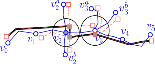
Figure 9: Here we see three paths in $H$ (pink dashed lines) stitched together to create a path close to a link-length five path in $G$ (blue solid lines).

Given a link-length $n$ vertex-path $p$ in $G$ for $n>4$, we show how to find a path in $H$ that is at most Fréchet distance $2(r_{d}+d)$ from $p$. Let $p$ be the path $v_{0}v_{1}\ldots v_{n-1}v_{n}$; for example, see Figure 9.

Vertices $v_{i}$ for $i=1,2,\ldots n-1$ must have degree at least four, since they are not end vertices and they are not of degree three. Therefore, for $i=2,3,\ldots,n-2$, we can choose a vertex $u_{i}$ adjacent to $v_{i}$ so that there exists at least one vertex between $u_{i}$ and $v_{i+1}$ in both a clockwise and a counter-clockwise ordering around $v_{i}$. Likewise, we can also choose a vertex $w_{i}$ adjacent to $v_{i}$ so there exists at least one vertex between $w_{i}$ and $v_{i-1}$ in both a clockwise and counter-clockwise ordering around $v_{i}$ for $i=2,3,\ldots,n-2$. For example, in Figure 9, $u_{2}=v_{1}$, $w_{2}=v_{3}$, $u_{3}=v_{3}^{a}$ and $w_{3}=v_{3}^{b}$. We define a set of paths that covers $p$. The first path we consider is $p_{1}=v_{0}v_{1}v_{2}w_{2}$. The last path is $p_{n-2}=u_{n-2}v_{n-2}v_{n-1}v_{n}$. In between, for each edge $v_{i}v_{i+1}$, we add the path $p_{i}=u_{i}v_{i}v_{i+1}w_{i+1}$. Notice that each path corresponds to one edge in $p$, except the first and last paths, which each correspond to two edges.

Next, we Fréchet-match $p_{i}$ in $G$ to $p_{i}^{\prime}$ in $H$ for $i=1,2,\ldots,n-2$, and perform surgeries on these paths in order to find a path $p^{\prime}$ in $H$ that is close to $p$. Notice that for each $i$, the Fréchet distance between $p_{i}$ and $p^{\prime}_{i}$ is at most $d$. Let $M_{i}$ be the Fréchet-correspondence from $p_{i}$ to $p^{\prime}_{i}$.

At each vertex $v_{i}$ for $i=2,3,\ldots,n-2$, we find $v_{i}^{\prime}$ and perform surgeries between $p_{i-1}^{\prime}$ and $p_{i}^{\prime}$, as described in Theorem 3.13 for $v_{2}$. We notice that the induced correspondences between paths after surgery are consistent with the correspondences before surgery for the parts of $p$ outside of the balls of radius $r_{d}(v_{i})+d$ centered at $v_{i}$. Therefore, two adjacent vertices $v_{i}$ and $v_{i+1}$ separated by $2(r_{d}+d)$ can be combined by using the common correspondence on the part of the edge $v_{i}v_{i+1}$ that is outside of the balls of radius $r_{d}+d$ around $v_{i}$ and $v_{i+1}$. Letting $p^{\prime}$ denote the path in $H$ after surgery, we have $\delta_{F}(p,p^{\prime})\leq 2r_{d}+d$. Together with Lemma 3.2, this proves the claim.

Let $m$ and $n$ be the the total number of vertices and edges in $G$ and $H$, respectively. Assume further that the edges consist of $O(1)$ line segments. There are $|\Pi^{3}_{G}|\in O(m^{3})$ paths of link-length three in $G$, and their total complexity is $O(m^{4})$. Using the map-matching algorithm of aerwMPM03, $\overrightarrow{d}_{path}(\Pi^{3}_{G},\Pi_{H})$ can be computed in $O(m^{4}n\log^{2}n)$ time, and from Theorem 3.15 follows that $\overrightarrow{d}_{path}(\Pi_{G},\Pi_{H})$ can be approximated in the same time.

If all edges in $G$ are line segments, then the total complexity of all link-length three paths in $G$ is $O(m^{3})$, and Lemma 3.8 and Theorem 3.15 yield the following:

Corollary 3.17 (Approximation).

If all edges in $G$ are line segments, no vertex in $G$ is of degree three, and the distance between any two adjacent vertices is at least $2\Delta_{3}(1+1/\sin(\theta/2))$, where $\theta$ is the smallest angle formed by two incident edges. Then $\overrightarrow{d}_{path}(\Pi_{G},\Pi_{H})\leq 2\Delta_{3}(1+1/\sin(\theta/2))$, and this approximation can be computed in $O(m^{3}n\log^{2}n)$ time.

In order to prove Theorem 3.10 (Crossing Paths) and Theorem 3.15 (Link-Length Three is Sufficient), we needed to use the assumption that all intersections are of degree four or more. The reason we need to assume this is in order to obtain a vertex correspondence. By using link-length two paths in $G$, we can find two transverse paths in $H$ and hence an intersection.

When the vertices have degree three, then the link-length two paths can be close without an intersection occurring. Figure 10a is an example of such occurrence with one degree three vertex. Figures 10b and 10c show a contrived example where $\overrightarrow{d}_{path}({\Pi^{3}}_{G},\Pi_{H})$ is small but path-based distance can be arbitrarily large. The closest correspondence of the bold path in $G$ is the bold path in $H$ and their Fréchet distance can not be bounded using link-length three paths.

In Section 4, we observe that vertices of degree three are common in road networks; see Tables 4.1 and 4.1. However, despite the datasets not meeting the assumptions of our theorems, we still can use the path-based distance to capture differences between the graphs. In particular, we observe that there are two main types of dissimilarities between graphs from real city data: missing turns and missing streets. Both of these differences can be identified using (edge or vertex) signatures; see Figure 5 and Figure 6. Next, we define these signatures.

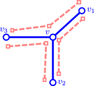
(a) Missing Intersection

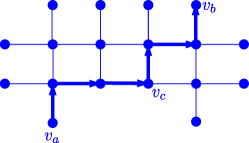
(b) Graph $G$

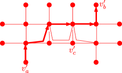
(c) Graph $H$

Figure 10: A vertex correspondence can not be guaranteed for a degree three vertex. (a) The blue and the pink graphs have a small path-based distance, however no vertex in the pink graph corresponds to $v$. The graph $G$ in blue (b) and $H$ in red (c) illustrate an example where $\overrightarrow{d}_{path}(\Pi_{G}^{3},\Pi_{H})$ is very small, but the path-based distance can be arbitrarily large. The closest correspondence of the bold path in $G$ is the bold path in $H$.

3.4 Path-Based Signature

One benefit of the path-based distance measure is that there is a natural local signature that can be defined. Given an edge $e\in E_{G}$, we ask what is a tight upper bound for the Fréchet distance of paths going through that edge? For a connected graph, this would be a constant value, if we do not restrict the types of paths that we consider. Instead, we look at paths of a fixed link-length $k$. For an edge $e\in E_{G}$ and for a given integer $k\geq 1$, the quantity $\Delta_{k,e}=\overrightarrow{d}_{path}(\Pi_{e}^{k},\Pi_{H})$ captures the distance of all link-length $k$ paths through $e$. In that sense, it represents a local signature for the edge $e$ describing the local structural similarity of a sub-graph centered at $e$ to a subgraph in $H$. This local signature can now be used to identify how well portions in $G$ correspond to portions in $H$. In Subsection 4.3, we provide two approaches for using this signature: First, we compute heat-maps that map the value of the signature onto the graph edges, in order to visualize the degree of local similarity captured by the signature. Second, we summarize the local signatures in a cumulative distribution function in order to capture a summary of the local graph similarity.

Note that a signature could also be defined for each vertex $v$ by considering $\Delta_{k,v}$, however for visualization purposes and for capturing the overall length of all edges in the graph, it appears more suitable to use $\Delta_{k,e}$.

4 Experimental Results

In this section, we present our experimental results. We implemented Java code to compute the path-based distance defined above. Besides using real street-maps from Berlin and Athens we used a set of perturbed graphs to analyze our distance measure; see Subsection 4.4. Our code is available on mapconstruction.org.

4.1 Datasets and Runtimes

We test our algorithm using map data from Berlin and Athens. For Berlin, we have maps from two sources: TeleAtlas (TA) from 2007 and OpenStreetMap (OSM) from April 2013. We have both small (16 km²) and large (2500 km²) maps of Berlin. Similarly, for Athens, we have TA maps from 2007 and OSM maps from 2010. To compute the path-based distance, we selected several rectangular regions with the same coordinates from each map; Table 4.1 contains the UTM coordinates of the southwest-most and northeast-most corners of the rectangular regions, and Tables 4.1 and 4.1 contains some statistics about the datasets. From these tables, we see that the OSM Berlin maps contain more vertices and edges than the TA maps; however, the OSM Athens-small map contains slightly fewer vertices and edges than the TA map.

Data Set Regions. Data set xLow xHigh yLow yHigh Area Athens-small $480,000$ m $484,000$ m $4,206,000$ m $4,210,000$ m $4$ km $\times$ $4$ km Berlin-small $390,000$ m $394,000$ m $5,817,000$ m $5,821,000$ m $4$ km $\times$ $4$ km Berlin-large $375,000$ m $425,000$ m $5,775,000$ m $5,825,000$ m $50$ km $\times$ $50$ km The data set regions are defined by the extreme southwest $(xLow,yLow)$ and the extreme northeast $(xHigh,yHigh)$ UTM coordinates.

Statistics for OSM maps. # vertices # edges total length all $degree\neq 3$ Athens-small 2,318 1,026 3,758 323 km Berlin-small 2,166 841 3,051 267 km Berlin-large 87,395 31,777 123,863 17,552 km

Statistics for TA maps. # vertices # edges total length all $degree\neq 3$ Athens-small 2,770 1,210 4,343 339 km Berlin-small 1,507 634 2,303 227 km Berlin-large 49,605 19,897 72,650 10,426 km

Runtimes. Dataset Link Teleatlas OSM to Execution Machine Length to OSM Teleatlas Mode Specification LinkOne 4.9 min 6.1 min Athens-small LinkTwo 22.0 min 27.8 min Intel(R) Xeon(R) LinkThree 74.9 min 98.4 min sequential CPU E3-1270 v2 LinkOne 5.8 min 5.6 min $@3.5GHz$ $8GB$ Ram Berlin-small LinkTwo 24.4 min 22.0 min LinkThree 78.4 min 69.0 min LinkOne 4.0 h 4.5 h http://www.cbi.utsa.edu/ Berlin-large LinkTwo 15.0 h 20.0 h parallel hardware/cluster LinkThree 49.0 h 53.0 h

The path-based algorithm for computing the distance between two maps is scalable and has reasonable runtime; for the Berlin-small dataset, it took $24.4$ minutes to map all link-length two paths of OSM to the TeleAtlas map. The runtime and machine specification for corresponding experiments are summarized in Table 4.1. Although this algorithm does not need to run in real-time, the computation can be sped up by incorporating an efficient data structure for spatial search. As the runtime is not our main focus in our current implementation, we perform an exhaustive search to find all points on the street-map which are close to the start vertex of a path.

The algorithm can be trivially parallelized by decomposing the set of paths in the first graph into multiple sets and finding their (Fréchet-)closest paths in the second graph independently. We implemented this parallel version of the path-based distance computation. For the Berlin-large dataset, there were almost $50,000$ paths to consider. When we executed the parallel computation, we used $25-250$ threads, resulting in runtimes listed in Table 4.1. This simple parallelization allowed for the path-based distance to be computed on the Berlin-large map in only two days time, as opposed to taking weeks to compute.

4.2 Computing the Path-Based Distance

The results presented in Section 3 require that the graphs are $d$-separated and that no vertex is of degree three. In the datasets that we use in this section, $55-64\%$ of the vertices have degree three; see Tables 4.1 and 4.1. If we relax the degree three condition, then we can compare paths in one graph to the (Fréchet-)closest path in the other graph. In our experiments, we allow degree three vertices, at the cost of having a slightly less informative distance measure. As discussed in Subsection 3.3, even though there are contrived examples for which the approximation guarantees of our theorems do not apply, we can still use the path-based distance to capture differences between the graphs.

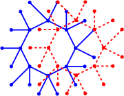
(a) Spatial.

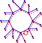
(b) Topological.

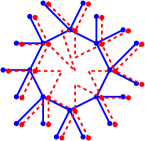
(c) Geometric.

Figure 11: Three typical examples where vertices that are not well-separated may arise: when one graph is a translation of the other, when one graph has more topological structure than the other, and when seemingly corresponding edges (according to the topology of the graphs) have very different geometric embeddings.

We look to Figures 11 and 3 to understand the settings for which vertices are not well-separated. Figure 11 shows three generic examples: poor separation due to spatial, topological, or geometric differences in the graphs. In practice, we see regions of well-separated vertices and regions of vertices that are not well-separated; see Figure 3.

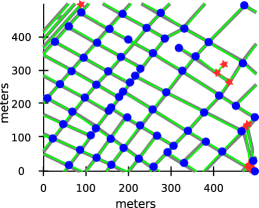
(a) Mostly well-separated region.

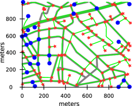
(b) Mostly not well-separated region.

Figure 12: We plot portions of the OSM and TA maps for the Athens-small dataset. The $\Delta_{3}$-separated vertices are displayed as blue circles and the other vertices as red stars. In (a), we see OSM (green) overlayed on TA (gray) where the road networks are very similar. In (b), we see TA (green) overlayed on OSM (gray) where the TA map has more streets than the OSM one, resulting in a large number of vertices that are not $\Delta_{3}$-separated.

When the vertices are not $d$-separated for sufficiently small $d$, then discerning the topological structure of the individual maps – let alone the differences between them – becomes difficult. For our three datasets, we counted the number of $d$-separated vertices for $d=\Delta_{1},\Delta_{2}$ and $\Delta_{3}$; see Table 4.2. If we look at $\Delta_{1}$-separated vertices for the Berlin-small dataset, we see that $54\%$ ($1,159$ out of $2,166$) vertices are well-separated. Similarly, we found that $76\%$ of the TeleAtlas vertices in Berlin-small are $\Delta_{1}$-separated.

Statistics about well-separated vertices. # vertices #$d$-separated vertices Dataset $d$ OSM Teleatlas OSM Teleatlas $\Delta_{1}$ 2,076 $\left(90\%\right)$ 2,020 $\left(73\%\right)$ Athens-small $\Delta_{2}$ 2,318 2,770 1,803 $\left(78\%\right)$ 1,616 $\left(58\%\right)$ $\Delta_{3}$ 1,490 $\left(64\%\right)$ 1,215 $\left(44\%\right)$ $\Delta_{1}$ 1,159 $\left(54\%\right)$ 1,149 $\left(76\%\right)$ Berlin-small $\Delta_{2}$ 2,166 1,507 811 $\left(37\%\right)$ 897 $\left(60\%\right)$ $\Delta_{3}$ 510 $\left(24\%\right)$ 665 $\left(44\%\right)$ $\Delta_{1}$ 38,402 $\left(44\%\right)$ 34,723 $\left(70\%\right)$ Berlin-large $\Delta_{2}$ 87,395 49,605 27,445 $\left(31\%\right)$ 32,344 $\left(65\%\right)$ $\Delta_{3}$ 18,898 $\left(22\%\right)$ 24,963 $\left(50\%\right)$

(a) $\Delta_{1}$

(b) $\Delta_{2}$

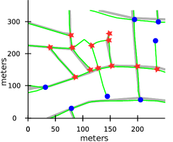
(c) $\Delta_{3}$

Figure 13: We demonstrate how a region of vertices that are not $\Delta_{k}$-separated grows as $k$ increases. Here, we see TA (in green) overlayed on OSM (in gray) for a section of the Athens-small dataset. In blue circles, we mark the $\Delta_{k}$-separated vertices, and in red stars, we mark the vertices that are not $\Delta_{k}$-separated.

Since, in our theorems, $d$ depends on the directed path-based distance between two sets of paths (one from each graph), that implies that determining if a vertex is $d$-separated depends not only on the graph containing the vertex, but also on the second graph to which we compare it. Recall from Definition 3.9 that a vertex $v\in G$ is $d$-separated if $r_{d}$ is finite. As $d$ increases, the probability that $r_{d}$ is infinite also increases. As $\Delta_{k}$ is non-decreasing with respect to $k$, the number of vertices that are not well-separated also grows with $k$, as demonstrated in Figure 4 for a section of the Athens-small dataset.

In Table 4.2, we show the values of the path-based distance for our datasets. Since the path-based distance is defined as the maximum of map-matching distances, see Definition 3.1, it is dominated by the most dissimilar sections in the maps. We therefore also record the $90^{th}$ percentile and the mean value of the set of map-matching distances, weighted by the overall length of the paths. These quantities may be more suitable in practice as these are less sensitive to outliers than the maximum. The distribution of map-matching distances can provide insights into differences between the graphs; however, unless the assumptions of the theorems of Section 3 are satisfied, it will not guarantee vertex, edge, and intersection correspondences for every vertex, edge, and intersection.

We see in Table 4.2 that for Athens-small, the distance from OSM to TA is consistently smaller than the distance from TA to OSM, which suggests that the TA map contains more detail than the OSM map. This behavior is reversed for Berlin-small and Berlin-large  where the distance from TA to OSM is consistently smaller, which suggests that the OSM map contains more detail. When considering the mean values, the Athens-small maps in particular appear to generally be in good correspondence, for one link, two link, and three link paths. For all data sets the effect of the different link-lengths is clearly noticeable: For the mean values highlighted in gray in Table 4.2, when increasing the link-length by one, the distances increase by $9-16$ meters for the small data sets, and by $24-32$ meters for the large data set.

Path-Based Distance. Path-based distance $90^{th}$-percentile Mean OSM TA to OSM TA to OSM TA to Datasets Path set to TA OSM to TA OSM to TA OSM $\Pi_{G}^{1}$ 150m 188m 11m 43m 8m 15m Athens-small $\Pi_{G}^{2}$ 157m 251m 42m 71m 17m 27m $\Pi_{G}^{3}$ 166m 251m 71m 96m 30m 45m $\Pi_{G}^{1}$ 203m 127m 70m 29m 25m 13m Berlin-small $\Pi_{G}^{2}$ 203m 130m 98m 61m 40m 24m $\Pi_{G}^{3}$ 210m 157m 121m 82m 63m 40m $\Pi_{G}^{1}$ $>1,600$m 1,150m 652m 57m $>204$m 26m Berlin-large $\Pi_{G}^{2}$ $>1,600$m 1,450m 896m 116m $>296$m 50m $\Pi_{G}^{3}$ $>1,600$m 1,450m 1095m 174m $>386$m 82m

When one map has more streets than the other, as is the case with the Berlin-large map, the path-based distance between them can be very large (as should be expected). Since the Berlin-large map contains part of the city of Berlin as well as parts of its southern suburbs (see Figures 1e and 1f), the local path-based distances observed by the edges and the vertices are not randomly distributed; there are regions in which the graphs are very similar, as well as regions where the graphs are dissimilar. For this reason, the value of the distance alone is difficult to interpret; therefore, we turn to the local signatures to provide more insight.

4.3 Using the Local Signature

In this subsection, we study the local signature $\Delta_{k,e}=\overrightarrow{d}_{path}(\Pi_{e}^{k},\Pi_{H})$ for a fixed $e\in E_{G}$ and for a given integer $k\geq 1$. We first show how heat-maps can be used as a visualization tool for the local similarity captured by the signature. This can help identify similar regions in the map. In a different approach, we then define a cumulative distribution function in order to capture a summary of the local signature in terms of percentage of the overall graph length.

Heat-Maps

We compute heat-maps by coloring an edge lighter shades of yellow to darker shades of red based on the value of that signature (smaller to larger). An edge $e\in G$ which is drawn in lighter shade implies correspondences in $H$ between $e$ and a subgraph induced by its neighborhood (depending on $k$) which is very similar spatially, structurally and topologically. On the other hand, a darker red edge implies one or more possible dissimilarities: missing edge, missing vertex, spatial/structural differences, etc.

First, we demonstrate the special features link-length one, link-length two and link-length three signatures can capture. As was shown in Subsection 3.1, the value $\Delta_{1}$ can bound distances between edges and their corresponding paths, but fails to identify when a vertex (i.e., connection between two edges) is missing. In Figures 5 and 6, the heat-map of the TA map is overlayed on the OSM map (in gray) of Berlin-small. In Figure 5, we can see that edges which are in the TA map but do not have corresponding edges in the OSM map have a large directed distance (indicated by the red color), when signatures are computed using link-length one paths. At the same time, the link-length one signature fails to identify the difference between two edges that become close and two edges that intersect. This difference, however, can be identified using link-length two paths; see the regions inside the green boxes in Figure 6.

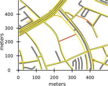
(a)

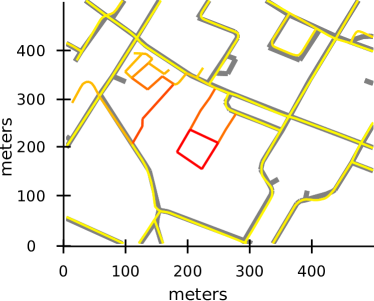
(b)

Figure 14: We plot the $\Delta_{1}$-signature of the TeleAtlas map, overlayed on the OpenStreetMap (in gray) for the Berlin-small dataset. TA edges with a close OSM path have a low signature and are shown in yellow. TA edges without any corresponding path in OSM have a high signature and are shown in red.

Although link-length two helps to find missing vertices, in some cases, it fails to capture differences in more global notions of connectivity. As one can see in the hypothetical example in Figure 16, $\Delta_{2}$ can be arbitrarily small with $\Delta_{3}$ arbitrarily large. Theorem 3.15 ensures that for $k>3$, the value of $\Delta_{k}$ cannot become arbitrarily larger than $\Delta_{3}$.

Cumulative Distribution of Local Signature Values

For a given edge $e\in E_{G}$ and a given integer $k\geq 1$, let $\Delta_{k,e}=\overrightarrow{d}_{path}(\Pi_{e}^{k},\Pi_{H})$ be the path-based signature at $e$. Similar to the distribution of $\Delta_{k,v}$ discussed above, the distribution of $\Delta_{k,e}$ provides insight into the similarity between $G$ and $H$. Therefore, we investigate this distribution in more detail. Given a distance threshold $x$ and a fixed link-length $k$, we define the weighted cumulative distribution of $\Delta_{k,e}$ as follows:

$$CDF(x;G,H,k)=\frac{\sum_{e\in E^{\prime}}\text{length}(e)}{\text{length}(G)},$$

where $E^{\prime}=\{e\leavevmode\nobreak\ :\leavevmode\nobreak\ \Delta_{k,e}\leq x\}$. In Figure 17, we plot $CDF(x;G,H,k)$ and $CDF(x;H,G,k)$ for three different data sets. We interpret these plots as follows: assume $y=CDF(x;G,H,k)$, then $y\%$ of the points in $G$ observe a path-based distance of at most $x$ meters.

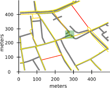
(a) $\Delta_{1}$-signature

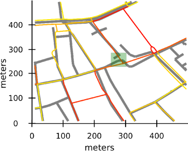
(b) $\Delta_{2}$-signature

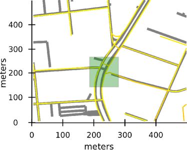
(c) $\Delta_{1}$-signature

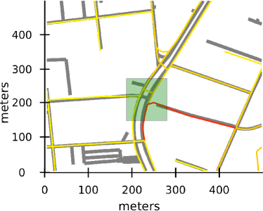
(d) $\Delta_{2}$-signature

Figure 15: We plot the path-based signature of the TeleAtlas map, overlayed on the OpenStreetMap (in gray) for the Berlin-small dataset. Note that $\Delta_{1}$ fails to capture missing vertices, but, as shown in the green boxes, $\Delta_{2}$ shows a large distance when the gray TA map has an intersection (in Figures (a) and (c)) which is missing in the colored OSM map (in Figures (b) and (d)).

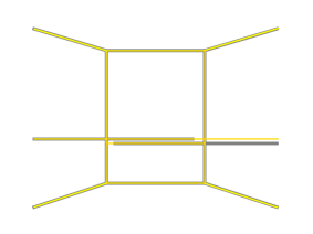
(a) $\Delta_{2}$-signature

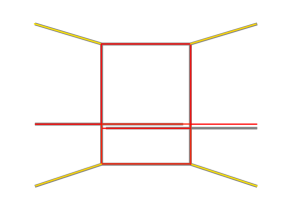
(b) $\Delta_{3}$-signature

Figure 16: $\Delta_{2}$ can be arbitrarily small with $\Delta_{3}$ arbitrarily large.

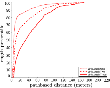
(a) Athens-small, TA mapped to OSM.

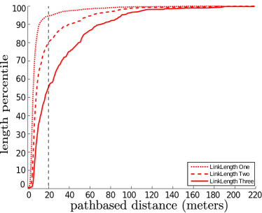
(b) Athens-small, OSM mapped to TA.

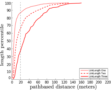
(c) Berlin-small, TA mapped to OSM.

(d) Berlin-small, OSM mapped to TA.

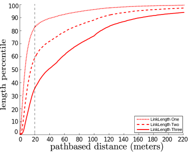
(e) Berlin-large, TA mapped to OSM.

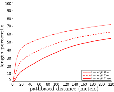
(f) Berlin-large, OSM mapped to TA.

Figure 17: For each point $p$ in a graph $G$, we assign to it the value $\Delta_{k,e}$, where $e$ is the edge containing $p$. Above, we plot the cumulative distribution of these assigned values. In particular, we take note of when the path-based distance is at most $20$ meters (indicated by the vertical gray lines), since the path-based distance exceeding $20$ meters indicates that the graphs are not similar near the edge $e$.

Figure 17d shows results for computing the distance from the 2013 OSM map to the 2007 TA map for Berlin-small. Here, we can see $68\%$ of the streets (more precisely, $181.56$ km out of $267$ km) have very close correspondence (less than or equal to $20$ meters) to the map of TA based on link-length one. That means that for $68\%$ of locations chosen in the OSM map, there exists a path in $H$ that has Fréchet distance at most $20$ meters to the edge containing the chosen location. Due to the large Fréchet distance to any path in the TA dataset, we can conclude that about $32\%$ of the streets in this area of Berlin were either omitted in the TA map or may have been new constructions between $2007$ and $2013$. This result is consistent with the observation in Section 4.2 that $54\%$ of the vertices are $\Delta_{1}$-separated. On the other hand, $85\%$ of the streets that existed in the 2007 map have a corresponding street in the 2012 map. New roads being built is a common occurrence, but removing roads is not. Since these street maps were taken from different sources, one explanation is that different types of roads can be ignored by OSM but would be recorded by TA.

Contrasting the Berlin-small dataset is the Athens-small dataset. In Athens-small, we see that $85\%$ of the streets from the 2007 TA map have corresponding link-length one paths in the 2010 OSM map, and $95\%$ of the OSM map have a corresponding path in the TA map. Perhaps some of this discrepancy can be explained by time. The Berlin road network had six years to change; whereas, the Athens dataset had only three years to change.

Looking at $CDF(x;H,G,k)$ for $k>1$ provides further insights. The cumulative distribution $CDF(x;H,G,1)$ gave information akin to Hausdorff distance. The distribution of $CDF(x;H,G,2)$ describes how well short distances (link-length two) are preserved between the graphs. The larger $k$ gets, the longer the paths are that need to be mapped from $G$ to $H$. In the Berlin-large dataset, only $81\%$, $57\%$ and $34\%$ of the TA can find paths close to all link-length one, two and three paths respectively. That also means $19\%$ of streets in TA are missing (or have dissimilar correspondence) in OSM, $81-57=24\%$ streets in TA are dissimilar to OSM because an adjacent turn and/or street is missing (similar to Figure 15d).

4.4 Experiments with Perturbed Data

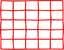
(a) $p=0.1$

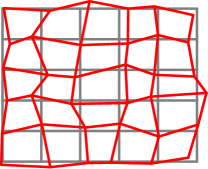
(b) $p=0.5$

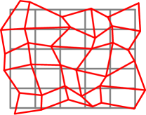
(c) $p=0.9$

Figure 18: The original $G$ is the grey graph, a regular grid over $\left[0,10\right]\times\left[0,10\right]$. As the perturbation index $p$ increases, the perturbation of vertices in a graph increases. The red graphs represent perturbed graphs for $p=0.1$, $0.5$ and $0.9$, from left to right.

In order to assess the ability of our distance measure to quantify dissimilarity between maps, we created a map $G$ and nine sets of estimations of that map with increasing allowable deviations from $G$. The map $G$ is a regular grid over $[0,10]\times[0,10]$ using the coordinates with even integers as the vertices; see the grey graph in Figure 18. The perturbation parameter is $p$, which is allowed to be between zero and one. We perturbed the vertex at $(i,j)$ in $G$ by choosing two numbers $\alpha$ and $\beta$ uniformly at random in the interval $[-p,p]$ and moving the vertex at $(i,j)$ to $(i+\alpha,j+\beta)$. Thus, as $p$ increases, the distance of the perturbed graph $G_{p}$ to the original graph $G$ should increase as well, in expectation. For each value $p$, we generate $100$ perturbed graphs: $G_{p}^{1},\ldots,G_{p}^{100}$. For example, see the red graphs in Figure 18 illustrating $G_{0.1}^{1},G_{0.5}^{1}$, and $G_{0.9}^{1}$.

Three sample maps. $p$ $\theta$ $\overrightarrow{d}_{path}(\Pi^{3}_{G_{p}},\Pi_{G})$ $\sqrt{2}p$ $0.1$ $83.00^{\circ}$ $0.125$ $0.14$ $0.5$ $55.43^{\circ}$ $0.695$ $0.71$ $0.9$ $29.83^{\circ}$ $1.195$ $1.27$

We first take a look at the three graphs in Figure 18. The values for $\theta$ and the distance $\overrightarrow{d}_{path}(\Pi^{3}_{G_{p}^{1}},\Pi_{G})$ are listed in Table 4.4. We observe that when increasing the perturbation parameter $p$, the angle $\theta$ decreases. Hence, the upper bound for $\overrightarrow{d}_{path}(\Pi^{3}_{G_{p}^{1}},\Pi_{G})$ from becomes quite large (for $G_{p}^{1}$ it is $0.628$ and for $G_{0.9}^{1}$ it is $11.675$). However, we notice that due to the perturbation scheme, $\overrightarrow{d}_{path}(\Pi^{3}_{G_{p}^{1}},\Pi_{G})\leq\sqrt{2}p$ since each coordinate can be perturbed by at most $p$. And, in fact, the link-three based distance is quite close to that bound.

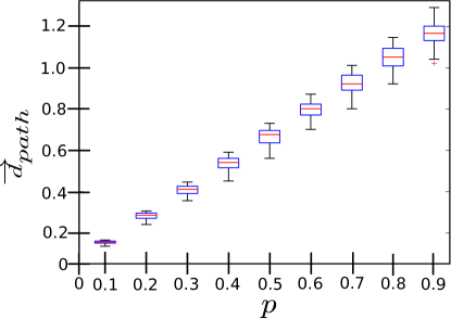
Figure 19: For fixed $p$, we show the boxplot for the distribution of observed distances. We can see as $p$ increases the path based distances increase as well. The path based distance captures dissimilarities at different levels.

We compute $\overrightarrow{d}_{path}({\Pi^{3}}_{G_{p}^{i}},\Pi_{G})$ for each $G_{p}^{i}$ and summarize our results in Figure 19, using boxplots to illustrate the distribution of path-based distances for each $p$. We observe that the path-based distance increases as the perturbation parameter $p$ increases, indicating that our distance measure can capture dissimilarities of varying levels. Graphs that are more similar (lower values of $p$) have the smallest distances, and graphs that are more dissimilar (higher values of $P$) have the largest distances.

4.5 Comparison with Biagioni and Eriksson 2012

In this section, we compare our distance measure with the sampling-based distance measure presented in Subsection 2.1. We used the code provided by Biagioni:2012:MIF:2424321.2424333, making modifications to allow for a different input format as well as to make the output comparable to the path-based signature presented in this paper. In particular, we take vertices (including degree two) from a graph as the seed locations instead of the random sampling used in [Biagioni and Eriksson (2012)]. The resulting marbles and holes distance ($F$-score) has three parameters:

1. Sampling density: how densely the map should be sampled (marbles for generated map and holes for ground-truth map); we use one sample every five meters.

2. Matched distance: the maximum distance between a matched marble-hole pair; we vary from $10$ to $220$ meters.

3. Maximum path length: from seed, the maximum distance from start location one will explore; we use $300$ meters.

Before commenting on the differences between the signatures, we first compare and contrast the $F$-score to the path-based distance. We compute the $F$-scores for the Berlin-small dataset by varying the matched distance from $10$ meters to $220$ meters, summarizing the results in Figure 20. Here, we can see the $F$-score is quite low and this finding is consistent with the observation we can draw from Figure 17d that $31\%$ of the roads in OSM Berlin-small map are new construction. Although the two Berlin-small maps do not look very dissimilar, the addition of more roads means that the topology of the maps has changed. Even if these changes are localized to a small area, the addition of topological features punishes the whole graph for being dissimilar in a tiny portion. Choosing the matched distance to be $20$ meters, the $F$-score is only $0.1265$. This computation took $17$ minutes, which is on the same order of magnitude as the computation of our distance measure.

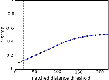
Figure 20: By increasing the matched distance threshold, the $F$-score also increases as it is easier for marbles and holes to be matched. This threshold is just one of the three parameters to the approach of Biagioni:2012:MIF:2424321.2424333.

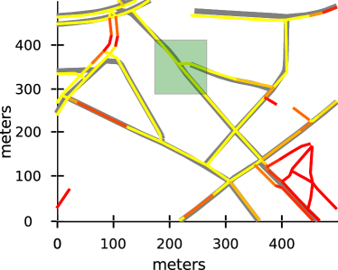
(a) $F$-score-signature

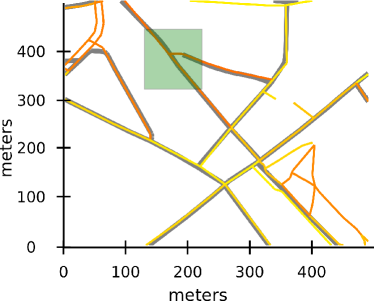
(b) $\Delta_{2}$-signature

Figure 21: OSM map overlayed on the TA map (in gray) for the Berlin-small dataset. The matched distance is $20$ meters. Note that the gray TA map has an intersection, while the colored OSM map does not. The $\Delta_{2}$ signature captures this as indicated by the darker orange color.

In order to compare two distance measures in a finer level, we compute $F$-scores for each start location individually and compute edge signatures by averaging the $F$-scores at the two endpoint vertices. We compute this $F$-score signature and plot its heat-map in an analogous fashion as we do for the path-based local signatures: we color an edge yellow if it observes similar behavior in both graphs (i.e., high $F$-score) and red if the distance indicates that the graphs are dissimilar (i.e., low $F$-score).

Balancing the tuning parameters above is difficult. Figure 21 shows a case where the graph sampling based distance measure fails to capture the difference between the two road networks due to the fact that the maximum path length was set too high. In gray, we plot the TA map, and we overlay that with the OSM map colored according to the adapted $F$-score in Figure 21a and our local signature in Figure 21b. In the green box, we notice that there is an intersection in the OSM map that is missing in the TA map, since one of the streets ends before it meets the other street. The $F$-score measure fails to identify the missing intersection since there is a detour available to reach the other road within $300$ meters of the seed (the intersection in the green box).

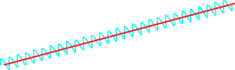
Figure 22: We consider evaluating the two distance measures on these two paths (taken to be graphs). In this example, one graph is straight and the second graph oscillates frequently, but the deviation from the straight line path is relatively small. Hence, the path-based distance is small indicating that the graphs are very close, but the $F$-score will be close to zero indicating that the graphs are very dissimilar.

Again, as this distance measure is based on one-to-one correspondence, it picks up streets on the OSM map very clearly (in red), which are missing in the TA map; whereas our measure picks them based on their proximity to the nearest street (darker yellow to orange); see lower right corner of Figure 21. There are examples for which our distance measure would find the graphs to be similar, but the $F$-score would be very low indicating that the graphs are not similar. For example, consider Figure 22. The first graph (in orange) consists of exactly one straight line path. The second graph (in cyan) consists of one path close to the orange one, but oscilates frequently. Depending on the circumstances, one distance measure would be preferred over the other. If the exact distance of the path traveled matters (e.g., in computing the cost of transporting goods), then using the $F$-score may be preferred; whereas, if the topology of the map is important (e.g., when deciding if roads have been closed or new roads added), then the path-based distance would be preferred.

The above illustrates one of the strengths of our distance measure: no tuning parameters must be adjusted in order to get a meaningful distance measure. Moreover, we have theoretical guarantees that capture the difference in navigation patterns between the two graphs.

5 Conclusion and Future Work

In this paper, we formally defined a path-based distance measure for the comparison of street map graphs. We provided a polynomial-time algorithm to approximate this distance, by approximating the maximum Fréchet distance over an infinite collection of pairs of paths. This is the first distance measure for comparing street maps that gives theoretical quality guarantees to compare travel paths between the street maps, and which can be approximated in polynomial time.

Summarizing the differences between the maps with a single number gives a global view of the differences, which may not provide enough detail about those differences. In general, finding correspondences between regions (or paths) of the street maps is a challenging task in map comparison. In this paper, we defined a vertex-based as well as an edge-based local signature, which allows for a natural visualization of the path-based distance. These local signatures provide the means to distinguish similar regions, as well as dissimilar regions, between two street maps.

We have made the code for computing our path-based distance available on www.mapconstruction.org, a website recently established for benchmarking map construction algorithms. The largest current comprehensive comparison of map construction algorithms using different distance measures is provided in [Ahmed et al. (2014b)]. Among the distance measures used is the path-based distance defined in this paper.

The work on the path-based distance measure has exposed several ideas warranting further investigation. The major constraint on the theoretical side was the exclusion of degree-three vertices. However, we have noticed that in practice the link-length three distance measure appears to accurately capture similarities and differences between maps. To close the gap between theory and practice, we ask what can be proven about path-based distances between networks that include degree-three vertices?

As mentioned in Section 2, finding the closest path in $H$ given a path $p$ in $G$ is called map-matching. Using the Fréchet distance to define closest is just one of the ways that this can be done. One of the limiting factors in this framework is that the Fréchet distance captures the worst-case behavior. In the future, we will investigate different map-matching techniques. We further plan on studying the use of alternative input models for the graphs, including directed graphs and non-planar graphs that can model bridges and tunnels. In addition, instead of using link-length three paths, we wonder if we can find a different set of paths that allows us to prove tighter approximation bounds.

To date, there are only a few approaches for comparing planar embedded graphs, and the definition of such distance measures varies depending on the context. Although this paper provides a new means of comparing road networks, there is still a need to develop more techniques for road network comparison.

This work has been supported by the National Science Foundation grants CCF-0643597 and CCF-1216602. We thank Dieter Pfoser for providing the TeleAtlas maps, Sophia Karagiorgou for helping with data conversion, James Biagioni for providing his code, and the anonymous referees for providing thoughtful feedback.

October 2014February 2015

References

- [1]
- A. and Madhvanath (2014) Bharath A. and Sriganesh Madhvanath. 2014. Allograph Modeling for Online Handwritten Characters in Devanagari Using Constrained Stroke Clustering. ACM Transactions on Asian Language Information Processing 13, 3 (2014), 12:1–12:21.
- Aanjaneya et al. (2011) Mridul Aanjaneya, Frederic Chazal, Daniel Chen, Marc Glisse, Leonidas J. Guibas, and Dmitriy Morozov. 2011. Metric Graph Reconstruction from Noisy Data. In Proc. ACM SoCG. 37–46. DOI:http://dx.doi.org/10.1145/1998196.1998203
- Ahmed et al. (2014a) Mahmuda Ahmed, Brittany Terese Fasy, and Carola Wenk. 2014a. Local Persistent Homology Based Distance Between Maps. In SIGSPATIAL. ACM.
- Ahmed et al. (2014b) Mahmuda Ahmed, Sophia Karagiorgou, Dieter Pfoser, and Carola Wenk. 2014b. A Comparison and Evaluation of Map Construction Algorithms. (2014). ArXiv preprint 1402.5138.
- Ahmed and Wenk (2012) Mahmuda Ahmed and Carola Wenk. 2012. Constructing Street Networks from GPS Trajectories. In Proc. European Symp. Algorithms. 60–71.
- Alt et al. (2003) Helmut Alt, Alon Efrat, Günter Rote, and Carola Wenk. 2003. Matching Planar Maps. J. Algorithms (2003), 262–283.
- Alt and Godau (1995) Helmut Alt and Michael Godau. 1995. Computing the Fréchet Distance between Two Polygonal Curves. Int. J. Comput. Geom. and Applications 5 (1995), 75–91.
- Biagioni and Eriksson (2012) James Biagioni and Jakob Eriksson. 2012. Map Inference in the Face of Noise and Disparity. In Proc. 20th ACM SIGSPATIAL. 79–88. DOI:http://dx.doi.org/10.1145/2424321.2424333
- Chen et al. (2010) Daniel Chen, Leonidas Guibas, John Hershberger, and Jian Sun. 2010. Road Network Reconstruction for Organizing Paths. In Proc. ACM-SIAM Symp. on Discrete Alg. 1309–1320.
- Cheong et al. (2009) Otfried Cheong, Joachim Gudmundsson, Hyo-Sil Kim, Daria Schymura, and Fabian Stehn. 2009. Measuring the Similarity of Geometric Graphs. In SEA. 101–112.
- Conte et al. (2004) Donatello Conte, Pasquale Foggia, Carlo Sansone, and Mario Vento. 2004. Thirty Years Of Graph Matching In Pattern Recognition. Int. J. Pattern Recognit. Artificial Intell. 18, 3 (2004), 265–298.
- Eppstein (1995) David Eppstein. 1995. Subgraph Isomorphism in Planar Graphs and Related Problems (SODA). SIAM, Philadelphia, PA, USA, 632–640. http://dl.acm.org/citation.cfm?id=313651.313830
- Ge et al. (2011) Xiaoyin Ge, Issam Safa, Mikhail Belkin, and Yusu Wang. 2011. Data Skeletonization via Reeb Graphs. In 25th Annual Conf. Neural Info. Proc. Sys. 837–845.
- Karagiorgou and Pfoser (2012) Sophia Karagiorgou and Dieter Pfoser. 2012. On Vehicle Tracking Data-Based Road Network Generation (SIGSPATIAL ’12). ACM, New York, NY, USA, 89–98. DOI:http://dx.doi.org/10.1145/2424321.2424334
- Kim et al. (1996) Hang Joon Kim, Jong Wha Jung, and Sang Kyoon Kim. 1996. On-line Chinese Character Recognition Using ART-based Stroke Classification. Pattern Recogn. Lett. 17, 12 (Oct. 1996), 1311–1322. DOI:http://dx.doi.org/10.1016/0167-8655(96)00078-5
- Liu et al. (2012) Xuemei Liu, James Biagioni, Jakob Eriksson, Yin Wang, George Forman, and Yanmin Zhu. 2012. Mining Large-Scale, Sparse GPS Traces for Map Inference: Comparison of Approaches (KDD). ACM, New York, NY, USA, 669–677. DOI:http://dx.doi.org/10.1145/2339530.2339637
- Mondzech and Sester (2011) Juliane Mondzech and Monika Sester. 2011. Quality Analysis of OpenStreetMap Data Based on Application Needs. Cartographica 46 (2011), 115–125.
- Shi et al. (2003) Daming Shi, Robert I. Damper, and Steve R. Gunn. 2003. Offline Handwritten Chinese Character Recognition by Radical Decomposition. 2, 1 (March 2003), 27–48. DOI:http://dx.doi.org/10.1145/964161.964163