Sub-arcsec Observations of NGC 7538 IRS 1: Continuum Distribution and Dynamics of Molecular Gas

Abstract

We report new results based on the analysis of the SMA and CARMA observations of NGC 7538 IRS 1 at 1.3 and 3.4 mm with sub-arcsec resolutions. With angular resolutions $\sim$ 0$\farcs$7, the SMA and CARMA observations show that the continuum emission at 1.3 and 3.4 mm from the hyper-compact H II region IRS 1 is dominated by a compact source with a tail-like extended structure to the southwest of IRS 1. With a CARMA B-array image at 1.3 mm convolved to 0$\farcs$1, we resolve the hyper-compact H II region into two components: an unresolved hyper-compact core, and a north-south extension with linear sizes of $<270$ AU and $\sim$2000 AU, respectively. The fine structure observed with CARMA is in good agreement with the previous VLA results at centimeter wavelengths, suggesting that the hyper-compact H II region at the center of IRS 1 is associated with an ionized bipolar outflow. We image the molecular lines OCS(19-18) and CH₃CN(12-11) as well as ¹³CO(2-1) surrounding IRS 1, showing a velocity gradient along the southwest-northeast direction. The spectral line profiles in ¹³CO(2-1), CO(2-1), and HCN(1-0) observed toward IRS 1 show broad redshifted absorption, providing evidence for gas infall with rates in the range of $3-10\times 10^{-3}$ M_⊙ yr^-1 inferred from our observations.

1. Introduction

NGC 7538 IRS 1 is a hyper-compact (HC) H II region located at a distance of 2.65 kpc (Moscadelli et al., 2009). Analysis of the radio and IR data suggested that IRS 1 is an O6/7 star with a luminosity of a few times of 10⁵ L_⊙ (Willner, 1976; Akabane & Kuno, 2005). High-resolution observations of IRS 1 with the Very Large Array (VLA) showed two lobes of free-free emission within the central 2″  region, located north and south of the emission peak of the HC H II region (Campbell, 1984; Gaume et al., 1995; Sandell et al., 2009). The centimeter emission has been interpreted as a north-south ionized jet/outflow, while the large-scale outflow in CO appears to be along the northwest-southeast direction (e.g. Scoville et al., 1986; Kameya et al., 1989; Davis et al., 1998; Qiu et al., 2011). At shorter wavelengths, a northeast-southwest elongation of dust emission was observed in the mid-IR (De Buizer & Minier, 2005) and at 0.87 mm, and several molecular lines show similar velocity gradients (Brogan et al., 2008; Klaassen et al., 2009; Beuther et al., 2012). In addition, a northwest-southeast linear structure of methanol masers with a velocity gradient of $\sim$0.02 km s^-1 AU^-1 was found by Minier et al. (1998, 2000). The kinematics from the methanol maser emission was modeled as a circumstellar disk (Pestalozzi et al., 2004) with a major axis in the northwest-southeast direction which is parallel to the axis of the large-scale outflow. Alternatively, the linear structure might be evident that the methanol masers trace the inner wall of an outflow instead of a disk (Pestalozzi et al., 2004). To reconcile the various models from the previous observations in CO, methanol masers, radio continuum and mid-IR emission, Kraus et al. (2006) proposed a precessing outflow model to interpret the observations.

In order to investigate the astrophysical process in the inner region of NGC 7538 IRS 1, we carried out high-angular resolution observations with the Submillimeter Array (SMA) at 1.3 mm and the Combined Array for Research in Millimeter-wave Astronomy (CARMA) at 1.3 and 3.4 mm. SMA archival data were also used in our analysis of the molecular lines and continuum emission from IRS 1. We present the results of the 1.3-mm and 3.4-mm continuum emission in Section 3 and molecular lines, including OCS(19-18), CH₃CN(12-11), CO(2-1), ¹³CO(2-1) and HCN(1-0), in Section 4. The implications of the results are discussed in Section 5. Section 6 summarizes the conclusions.

2. Observations and Data Reductions

2.1. SMA Data

SMA observations of NGC 7538 IRS 1 in the very-extended (VEX) configuration were made on 2008 August 5 with LO frequency $\nu_{\rm LO}$ = 226.239 GHz, giving band-center frequencies of 221 GHz for lower side band (LSB) and 231 GHz for upper side band (USB). Eight antennas were used in the observations with the longest projected baseline 339 $k\lambda$. The spectral resolution was 0.81 MHz, which corresponds to a velocity resolution of $\sim$1.1 km s^-1. The total on-source integration time was 82 minutes. The average system temperature was 180 K.

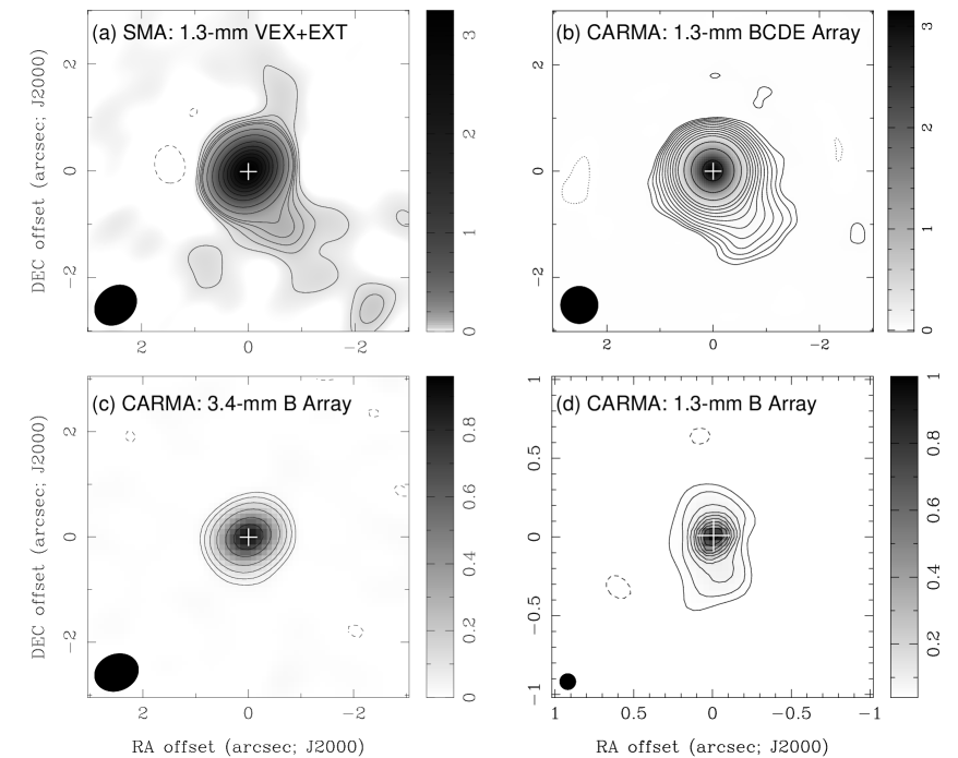
Figure 1.— (a) The SMA 1.3-mm continuum image made with the line-free channels by combining LSB and USB data from both VEX and EXT array observations. The contours are (–5, 5, 7, 10, 14, 20, 28, 40, 56, 80, 112, 160, 226, 320, 452, 640, 905, 1280)$\times\sigma$, and $\sigma=4$ mJy beam^-1. The FWHM beam size is 0$\farcs$8$\times$0$\farcs$6, P.A.$=-45$°. (b) The CARMA 1.3-mm continuum image with lower-resolution made by combining B, C, D and E array configuration data, convolved to a circular beam (FWHM) of 0$\farcs$7, with rms noise, $\sigma=2.5$ mJy beam^-1. The contours are (–4, 4, 5.7, 8, 11.3, 16, 23, 32, 45, 64, 91, 128, 256, 512 and 1028)$\times\sigma$. (c) The CARMA 3.4-mm continuum image made from the CARMA B-array observations with FWHM beam of 0$\farcs$8$\times$0$\farcs$7, P.A.$=-68$°. The contours are (–2, 4, 8, 16, 32, 64 and 96)$\times\sigma$. The rms noise $\sigma=$ 7 mJy beam^-1. In all the images the reference position is R.A. (J2000) = 23^h13^m45.^s37, Dec. (J2000) = 61$\arcdeg$28$\arcmin$10$\farcs$43, which is the peak position of 43 GHz continuum emission and marked by a plus. The FWHM of the synthesized beam is indicated at the left-bottom corner of each image. The greyscale of the wedges is in the units of Jy beam^-1. (d) The CARMA 1.3-mm continuum image of the centeral region of IRS 1 with a higher-resolution made with the B-array data only, convolved to a circular beam (FWHM) of 0$\farcs$1, and with rms noise, $\sigma=10$ mJy beam^-1. The contours are (–4, 4, 5.7, 8, 11.3, 16, 23, 32, 45, 64, 91)$\times\sigma$.

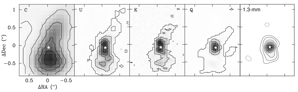
Figure 2.— The CARMA high-resolution image of IRS 1 at 1.3 mm is compared with the images observed with the VLA at 6, 2.0, 1.3 and 0.7 cm (Sandell et al., 2009). Different from other figures in this paper, this reference center is the same as the original figure in Sandell et al. (2009). The white stars mark the position R.A. (J2000) = 23^h13^m45.^s37, Dec. (J2000) = 61$\arcdeg$28$\arcmin$10$\farcs$43.

NGC 7538 IRS 1 was also observed with the SMA in the extended (EXT) configuration on 2005 September 11, with an LO frequency $\nu_{\rm LO}$ = 226.348 GHz. Six of the eight SMA antennas were used, giving the longest projected baseline 133 $k\lambda$. A standard correlator configuration was used with a spectral resolution of 0.33 MHz, corresponding to a velocity resolution of 0.42 km s^-1. The total on-source integration time was 309 minutes, and the average system temperature was 105 K.

The data reduction and analysis were made in MIRIAD (Sault et al., 1995) following the reduction instructions for SMA data. For the EXT array data set (2005), system temperature corrections were applied to remove the atmospheric attenuation. Antenna-based bandpass solutions were calculated over three time intervals (UT 4:45-5:40 for Neptune, UT 6:00-6:30 and 14:00-14:45 for 3C454.3) to interpolate the corrections for the bandpass ripples due to instrument defects. After that, baseline-based and spectral-window based residual errors in bandpass were further corrected using the point source 3C454.3. The time-dependent gains were derived and interpolated from two nearby QSOs J0102+584 and J2202+422; the complex gain corrections were applied to the target source. Finally, the flux-density scale was bootstrapped from Ceres using the SMA planetary model assuming a flux-density of 0.95 Jy and an angular size of 0$\farcs$43. The reduction of the VEX array data is similar, and the calibrators used in the data reduction for the EXT and VEX configuration data are summarized in Table 1.

In order to image the continuum emission and the molecular lines in the IRS 1 region with high angular resolution and good uv coverage, we combined the EXT (2005) and VEX (2008) datasets. The EXT and VEX visibility datasets have an offset of 0$\farcs$7 in pointing position. Using UVEDIT in MIRIAD, we shifted the two data sets to a common phase reference center at the continuum peak position determined from the EXT (2005) data set. Then, the residual phase errors in the continuum were further corrected using the self-calibration technique with a point-source model at the position of the radio compact source in IRS 1 determined from the VLA image at 43 GHz (Sandell et al., 2009). The self-calibration solutions determined from continuum data were also applied to the line data sets.

The continuum data sets were created by averaging all the line-free channel data using UVLIN. Combining the USB and LSB datsets of the EXT and VEX array configurations, the continuum image at 1.3 mm was constructed. The continuum-free line visibility data sets were created by subtracting the continuum level determined from a linear interpolation from the line-free channels using UVLIN in MIRIAD.

In addition to the 1.3-mm results, we also included the SMA data of NGC 7538 IRS 1 at 345 GHz which were observed in 2005 (Brogan et al., 2008). The FWHM beam sizes for the final line images are about 2″. We analyzed the relatively optically thin lines of species CH₃OH and ¹³CH₃OH to determine the systemic velocity of the IRS 1 system.

2.2. CARMA Data

2.2.1 1.3 mm

High-resolution observations of IRS 1 were carried out on January 4 and 5, 2010 with CARMA in the B array configuration at 1.3 mm. The CARMA observations used two 500 MHz bands in upper and lower sidebands of LO1 with a total continuum bandwidth of 2 GHz. The data were reduced and imaged in a standard way using MIRIAD software. The quasar J0102$+$584 was used as a gain and phase calibrator, and Uranus and MWC 349 for flux and bandpass calibration. The uncertainty in the absolute flux-density scale was $\sim$20%. The strong compact emission from IRS 1 was used to self-calibrate IRS 1 with respect to the 43 GHz VLA image with a Gaussian fit position R.A. (J2000) = 23^h13^m45.^s37, Dec. (J2000) = 61°28′10$\farcs$4. The continuum image was constructed by combining the two-500 MHz sidebands in a multi-frequency synthesis (MFS) mosiac. The CARMA data with three different primary beams resulting from the 6.1 and 10.4 m antenna pairs were used in the mosaic imaging. The weighted mean observing frequency from multi-frequency synthesis is 222.2 GHz.

To verify the structure observed with the SMA, we used the lower-resolution data from the CARMA observations in C, D and E array configurations that were carried out between 2007 to 2010. The setup of the corresponding observations are summarized in Table 1, giving observing date, pointing positions, band information, array configurations and calibrators of these observations. All of these observations were made with two or three 500-MHz wide bands in upper and lower sidebands with total bandwidths of 2 or 3 GHz. These continuum data were calibrated following the standard procedure. The calibrated datasets were split into single source datasets for the target source IRS 1. With UVEDIT, the phase-centers of each dataset were shifted to the common position of the IRS 1 continuum source determined from the VLA image at 43 GHz. Then, the residual complex gain errors in all the B, C, D and E array data sets were corrected using self-calibration with an initial model of a point source at the phase center. The structure seen in the B-array image which was self-calibrated with the model from the 43-GHz VLA image (as discussed in the above paragraph) was confirmed from this self-calibration procedure using a point-source as an initial model.

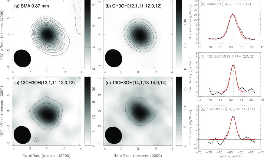
Figure 3.— (a) The SMA 0.87-mm continuum image with a FWHM beam size of 2$\farcs$1$\times$2$\farcs$0, P.A. $=38$°. The contours are (–1, 1, 2, 3, 4, 6, 8, 10, 12, 15, 18, 21, 24, 28)$\times$5$\sigma$, and the rms noise is $\sigma=45$ mJy beam^-1. (b) The integrated intensity map of the line CH₃OH(12,1,11-12,0,12) with a FWHM beam size of 2$\farcs$2$\times$2$\farcs$0, P.A. $=29$°. The contours are (-1, 1, 2, 3, 4, 5, 6, 7, 8)$\times$10$\sigma$, and the rms noise is $\sigma=1.7$ Jy beam^-1 km s^-1. (c) The integrated intensity map of the line ¹³CH₃OH(12,1,11-12,0,12) with a FWHM beam size of 2$\farcs$2$\times$2$\farcs$0, P.A. $=31$°. The contours are (-1, 1, 2, 3, 4, 5, 6, 7, 8)$\times$3$\sigma$, and the rms noise is $\sigma=1.7$ Jy beam^-1 km s^-1. (d) The integrated intensity map of the line ¹³CH₃OH(14,1,13-14,0,14) with a FWHM beam size of 2$\farcs$1$\times$2$\farcs$0, P.A. $=38$°. The contours are (-1, 1, 2, 3, 4, 5, 6, 7, 8)$\times$3$\sigma$, and the rms noise is $\sigma=2.0$ Jy beam^-1 km s^-1. (e) - (g) The spectra of CH₃OH(12,1,11-12,0,12), ¹³CH₃OH(12,1,11-12,0,12) and ¹³CH₃OH(14,1,13-14,0,14) at the peak position of the continuum emission. The red lines in (e) - (g) are the results of Gaussian fitting for the line profiles.

Figure 4.— The spectra toward IRS 1 that made from the upper (top) and lower (bottom) side bands based on the observations with the SMA on September 11, 2005 in the extended array configuration. The spectra have been converted to the rest frame at $V_{\rm sys}=-59.0$ km s^-1. The identifications for the major molecular and hydrogen recombination lines are labeled.

2.2.2 3.4 mm

We also carried out observations at 89 GHz with the CARMA telescope in the B array configuration with 15-antennas on December 28, 2010. We used a correlator setup with 16 spectral windows (including upper and lower sidebands), four with 500 MHz bandwidth (39 channels in total and 12.5 MHz for each channel), four with 250 MHz (79 channels in total and 3.225 MHz for each channel) and the remaining eight windows with 64 MHz bandwidth (255 channels in total and 0.244 MHz for each channel).

The data were calibrated and imaged following the standard procedure for CARMA data in MIRIAD. The HCN(1-0) line at $\nu_{0}=$88.6318 GHz was included in one of the narrow-band windows. The continuum data set was made from the line-free channels in this window. The residual phase errors were corrected using the self-calibration technique. The position of the IRS 1 continuum source at 3.4 mm was offset (–0$\farcs$18,–0$\farcs$10) from the SMA position at 1.3 mm, which is within the positional uncertainty in the SMA image. We binned two channels together to make a line image of HCN(1-0) with the same FWHM beam size as the continuum image.

A log summarizing the observations, uv datasets and images is given in Table 1.

3. Structure of Continuum Emission from IRS 1

With an angular resolution of $\sim$0$\farcs$7, both the SMA (Figure 1a) and CARMA (Figure 1b) show extended emission with a peak flux density of 0.12$\pm$0.02 Jy beam^-1, located $\sim$1″SW of the unresolved component in IRS 1. Lacking centimeter counterparts, the extended continuum emission is likely to correspond to thermal dust emission, which could contain additional dust cores in the IRS 1 region. It is also plausible that the SW extension corresponds to a dust component which is located along the interface between the ionized and molecular medium and is compressed by the ionized outflow.

The CARMA image at 3.4 mm (Figure 1c) shows a point-like source with no significant detection of the SW extension. A total flux density of 0.93$\pm$0.10 Jy was determined for the central unresolved core. Assuming a flat power-law ($\beta\sim 0.5$ for dust emissivity), a peak flux density of 0.01 Jy beam^-1 is extrapolated from the 1.3-mm peak flux density of the SW extension, which is below the 3$\sigma$ limit of the 3.4 mm-image.

The CARMA 1.3-mm image (Figure 1d), convolved to a circular beam of 0$\farcs$1, shows a central emission peak with a flux density of 1.0$\pm$0.1 Jy beam^-1. The innermost part of the HC H II region at 1.3 mm is un-resolved, which could be the optically thick part of the ionized outflow containing an accretion disk in IRS 1. Because the optically thick free-free emission dominates the 1.3-mm continuum, as well as the limitation of the angular resolution, the postulated ionized disk in IRS 1 has not been detected. In the CARMA 1.3-mm image (Figure 1d), extensions along the south and north directions from the bright point source has been revealed with a scale of 0$\farcs$8 above a noise level of 4 $\sigma$. The emitting lobes appear to be from the inner portion of the ionized outflow.

Previous studies show that the continuum emission from IRS 1 is dominated by the free-free emission from a bipolar ionized outflow at frequencies lower than 300 GHz (Sandell et al., 2009). Figure 2 compares the CARMA 1.3-mm image with previous VLA images. At wavelengths $\lambda\geq 1.3$ cm, a dark lane divides two emission peaks in the center of the IRS 1 region, which is probably due to the self-absorption in the ionized gas. At shorter wavelengths, $\lambda\leq 7$ mm, a single emission peak appears, located at R.A. (J2000) = 23^h13^m45.^s37, Dec. (J2000) = 61°28′10$\farcs$43. Hereafter, we take this position as the reference to register both the SMA and CARMA images.

The properties of the continuum sources in the IRS 1 region are summarized in Table 2.

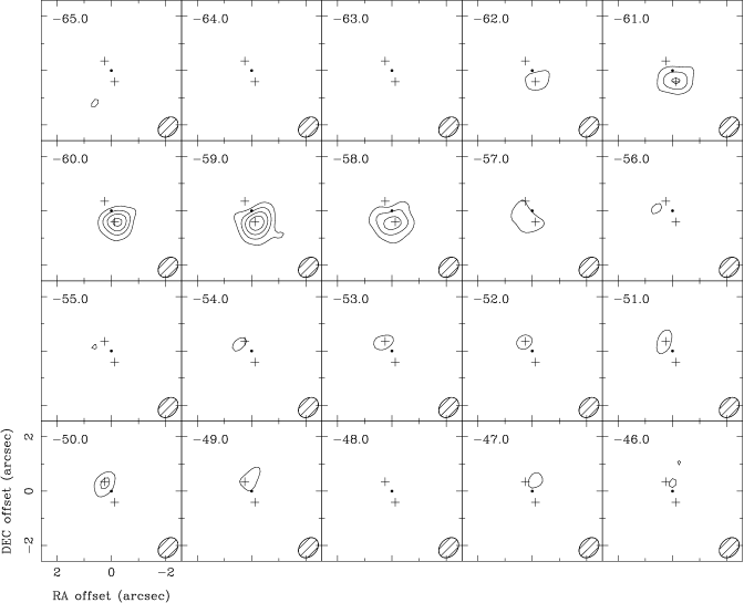
Figure 5.— The channel maps of the OCS(19-18) lines. The contours are (–1, 1, 2, 3, 4, …)$\times$5$\sigma$, and 1 $\sigma=0.06$ Jy beam^-1. The FWHM beam size is 0$\farcs$8$\times$0$\farcs$6, P.A.$=-43\arcdeg$. IRS 1 is located at the phase center (marked by filled black circles), and the intensity peaks of the SW and NE components are marked by plus signs.

4. Molecular lines

4.1. Systemic Velocity

At 1.3-mm wavelength, the SMA data for NGC 7538 IRS 1 show numerous strong molecular emission lines along with a few absorption features. A large portion of the emission is from the molecular lines with high excitation energy levels (e.g. OCS, CH₃CN, CH₃OCH₃ and C₂H₅OH), showing a strong emission peak at a radial velocity of $-59.5$ km s^-1 with a scatter of about one channel width ($\sim$0.5 km s^-1). This value is close to the velocity ($-59.7\pm 0.3$ km s^-1) observed in the mid-infrared by Knez et al. (2009). In addition, we further investigated the 0.86-mm SMA data and analyzed the CH₃OH(12,1,11-12,0,12), ¹³CH₃OH(12,1,11-12,0,12) and ¹³CH₃OH(14,1,13-14,0,14) lines. The integrated intensity images and line profiles are shown in Figure 3, and the Gaussian fitting to the line profiles are summarized in Table 3. The Gaussian fitting shows an average peak velocity of $-58.6\pm 0.2$ km s^-1 for these lines. These lines are with higher excitation energy than the ones observed in the 1.3-mm SMA data, as well as lower optical depths (for the two rare isotopic ones). On the other hand, since the $\sim$2″angular resolution of the 0.86-mm observations is poor compared to the 1.3-mm observations, it is possible that the 0.86-mm emission includes the kinematics of surrounding medium (e.g., outflow, infall). Therefore, considering the results of all the observations we adopt $V_{\rm sys}=-59.0\pm 0.5$ km s^-1, as the systemic velocity of the IRS 1 system in the following analysis.

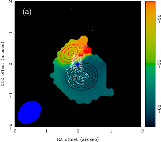
Figure 6.— (a) The integrated intensity maps of the OCS(19-18) components IRS 1 NE (red) and SW (black) superimposed on the centroid velocity image (color background). The velocity ranges of the integrations are ($-54.0$, $-47.0$) km s^-1 and ($-62.5$, $-57.0$) km s^-1 for IRS 1 NE and SW, respectively. The contour levels are (2.3, 2.8, 3.3) and (3.0, 3.8, 4.6, 5.4) Jy beam^-1 km s^-1 for IRS 1 NE and SW, respectively. The rms noise $\sigma$ is 0.15 Jy beam^-1 km s^-1. The FWHM beam size is 0$\farcs$8$\times$0$\farcs$6, P.A. $=-45$°. The unit of the wedge scaling is km s^-1. The white contours present the 1.3-cm continuum emission from the VLA observations (re-produced according to Gaume et al., 1995). IRS 1 is located at the phase center, marked by blue dot. Plus signs mark the peak positions of IRS 1 NE and SW in OCS(19-18). (b) The line profiles of OCS(19-18) at the peak positions of IRS 1 SW (solid line) and 1 NE (dashed line). (c) The line profile of OCS(19-18) integrated over the entire IRS 1 region.

4.2. Line Identifications of the 1.3-mm SMA Data

Figure 4 shows the spectra from the 1.3-mm SMA data observed in the EXT configuration, which are corrected for the systemic velocity, $V_{\rm sys}=-59.0$ km s^-1. Numerous molecular lines were identified on the basis of the molecular line surveys toward Sgr B2 (Nummelin et al., 1998) and Orion (Sutton et al., 1985), as well as other available line catalogs. The names of the identified molecules are labeled in Figure 4.

With no significant blending with other lines, OCS(19-18) and multiple $K$ transitions of CH₃CN(12-11) included in both EXT and VEX configuration observations were selected in our analysis to determine the excitation condition and kinematics in the IRS 1 region.

4.3. OCS(19-18)

The channel maps of the OCS(19-18) line show two significant velocity components in OCS(19-18) emission (see Figure 5). The main OCS(19-18) emission component in the velocity range from $-62.5$ to $-57.0$ km s^-1 is referred to as IRS 1 SW as it is located to the south and southwest of the HC H II region IRS 1, while the fainter, less extended redshifted component, hereafter IRS 1 NE, is located to the northeast of IRS 1 ranging from $-52.0$ to $-47.0$ km s^-1. No significant OCS(19-18) emission is present in the velocity range between $-56.5$ and $-53.0$ km s^-1. This velocity gap in emission is redshifted with respect to $V_{\rm sys}=-59.0$ km s^-1.

Figure 6a shows the integrated line intensity of the two components SW and NE. We fitted the two components with 2-D Gaussians as well as their line profiles with multiple Gaussians. The fitting results are summarized in Table 4. The peak position of IRS 1 SW is offset ($-0\farcs 13\pm 0\farcs 03$, $-0\farcs 41\pm 0\farcs 03$) with respect to IRS 1 while the offset of IRS 1 NE is ($0\farcs 25\pm 0\farcs 03$, $0\farcs 35\pm 0\farcs 02$). The total integrated line flux of OCS(19-18) for IRS 1 SW ($10.1\pm 0.7$ Jy km s^-1) is about three times of the value for IRS 1 NE ($3.8\pm 0.6$ Jy km s^-1).

Figure 6b shows the line profiles of the OCS(19-18) spectra at the peak positions of IRS 1 SW and NE, and Figure 6c shows the spectral profile integrated over the entire IRS 1 region. Gaussian fits to the observed spectral profiles give a radial velocity $V_{\rm LSR}=-59.5\pm 0.1$ km s^-1 with a line width $\Delta V_{\rm FWHM}=4.4\pm 0.1$ km s^-1 for IRS 1 SW, and $V_{\rm LSR}=-51.5\pm 0.3$ km s^-1 and $\Delta V_{\rm FWHM}=7.2\pm 0.6$ km s^-1 for the weaker emission feature (IRS 1 NE) (see Table 4). The centroid velocity of IRS 1 SW is close to $V_{\rm sys}=-59.0$ km s^-1 used in this paper, suggesting that ambient gas might dominate this component. The spectrum of IRS 1 NE is not a well-defined Gaussian shape, and the large line width suggests that it is subject to more dynamic interaction than IRS 1 SW.

Figure 7.— (a)-(b) The line profiles of CH₃CN(12-11), $K=0,1,2$ and $K=3,4,5,6,7,8$ at the intensity peak position of IRS 1 SW. The spectra are converted to $V_{\rm LSR}=-59.5$ km s^-1. The blending due to component NE is neglectable at this position. (c)-(d) The line profiles of CH₃CN(12-11), $K=0,1,2$ and $K=3,4,5,6,7,8$ at the intensity peak position of IRS 1 NE. The spectra are converted to $V_{\rm LSR}=-51.5$ km s^-1. In (c) the transition $K=0$ is blended with the transition $K=1$ from IRS 1 SW.

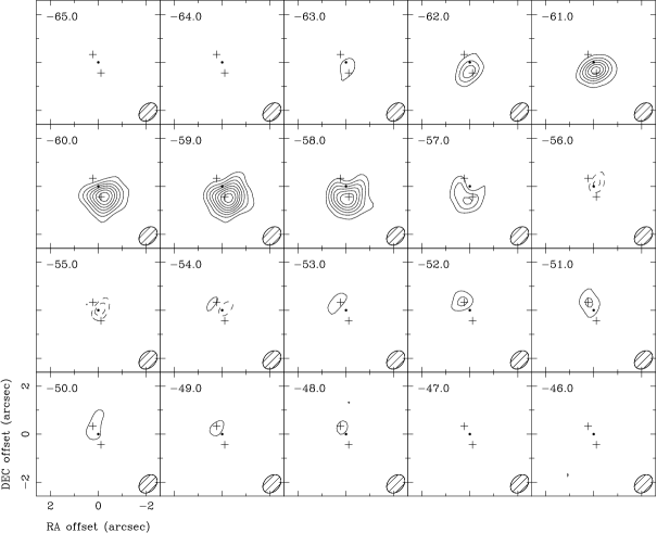
Figure 8.— The channel maps of CH₃CN(12-11) were constructed by combining the visibility data of $K$=2-5 transitions in the LSR velocity domain, which is equivalent to averaging the line intensities from the $K$=2-5 transitions. The contours are (–1, 1, 2, 3, 4, …)$\times$5$\sigma$, and 1 $\sigma=0.03$ Jy beam^-1. The FWHM beam size is 0$\farcs$8$\times$0$\farcs$6, $\rm P.A.=-45$°. IRS 1 is located at the phase center (indicated by filled black circles), and the intensity peaks of the SW and NE components are marked by plus signs.

4.4. CH₃CN(12-11) Lines

The CH₃CN(12-11) $K$-ladder with $K$=0-8, which covers the frequencies ranging from $\nu_{K=8}$ (220.476 GHz) to $\nu_{K=0}$ (220.747 GHz), were all detected in IRS 1 (see Figure 7). Similar to what is seen in OCS(19-18), the CH₃CN(12-11) lines also show an emission peak at $\sim-59.5$ km s^-1 with weaker redshifted components. At the intensity peak of IRS 1 SW, the line profiles of $K$=0-8 transitions are shown in Figure 7a and b, while as for IRS 1 NE, only $K$=0-7 transitions are detected above 3-$\sigma$ level. The $K$=0 and $K$=1 transitions, however, only have a frequency difference of 4.25 MHz ($\sim$5.8 km s^-1). We used double-component Gaussian models to fit the $K$=0, 1 line profiles for SW and NE respectively, which give uncertainties of 10% for SW and 15% for NE in line fluxes. Another issue is that the velocity separation between $K$=0 and 1 transitions is comparable to the velocity difference of the emission peaks toward SW and NE. With our sub-arcsec resolution, IRS 1 NE and SW are only marginally separated, therefore the blending of the main $K$=1 emission from IRS 1 SW with the redshifted $K$=0 emission from IRS 1 NE is expected. Due to the contamination caused by the blending, the transition of $K$=0 toward IRS 1 NE should be used with caution in the following analysis. As Figure 7b shows, the $K$=0 and $K$=2 transitions from IRS 1 SW are quite weak toward IRS 1 NE. Assuming that the main $K$=1 emission from IRS 1 SW has a similar intensity, we estimate that about 15% of the observed intensity of the redshifted $K$=0 emission toward IRS 1 NE is actually contributed by the blending from the main $K$=1 emission. Toward IRS 1 SW the error of the main $K$=1 emission due to the blending from the redshifted $K$=0 emission is negligible.

The intensity of the $K$=3 component for both IRS 1 NE and SW is abnormally low compared to the other $K$ components under the assumption that the CH₃CN components are in local thermal equilibrium (LTE), homogeneous and optically thin. As shown in Figure 7a and b for the SW component, the peak intensity of the $K$=0-4 transitions are nearly identical, indicating that the low $K$ transitions of CH₃CN in the SW component are optically thick. The optical depth of $K$=3 component is even higher due to its doubled statistical weight. Thus, the optically thick components must be excluded in the fitting for kinetic temperature with the assumption of optically thin and LTE (see Section 4.5).

In addition, we noticed that the intensity of the $K$=6 component toward IRS 1 NE is higher than the other components including $K$=3, 4, 5 and 7. This could be attributed to two causes. First, the $K$=6 component has a much higher column density than the components of $K$=4 and 5 due to its doubled statistic weight, but it still remains optically thin compared to the components of $K$=0, 1, 2 and 3. Second, the intensity of the $K$=6 component toward IRS 1 NE is likely to be affected by the line blending with HNCO(10_1,9-9_1,8) at rest frequency $\nu_{0}=220.5848$ GHz from SW and CH${}_{3}^{13}$CN(12₃-11₃) at $\nu_{0}=220.6000$ GHz from NE itself. From the comparison of Figure 7b and 7d, it seems that these possible line blending caused a non-zero baseline in the frequency range from 220.58 to 220.61 GHz toward NE, which might contribute up to 20% to the measured peak intensity of $K$=6 component of CH₃CN(12-11).

The possible blending from weaker molecular lines is also examined. We noticed that the line frequencies of C₂H₅OH are close to the $K$=1, 3 and 4 transitions of CH₃CN(12-11) and a CH₃OCHO-E line close to $K$=3 transition of CH₃CN(12-11). However, according to the JPL catalog, the typical intensities of those lines are only a few percent of the CH₃CN lines, and the contamination would produce no significant effects.

We constructed line images for each $K$ transition (not shown in this paper) and fitted the intensity peak positions for both the IRS 1 SW and NE components based on the integrated line flux images of $K$=0-8. We also fitted the line profiles of each $K$ transition to determine their peak intensities ($\Delta S_{\rm L}$), centroid velocity ($V_{\rm LSR}$) and FWHM line width ($\Delta V_{\rm FWHM}$). The derived values for these quantities are summarized in Table 4.

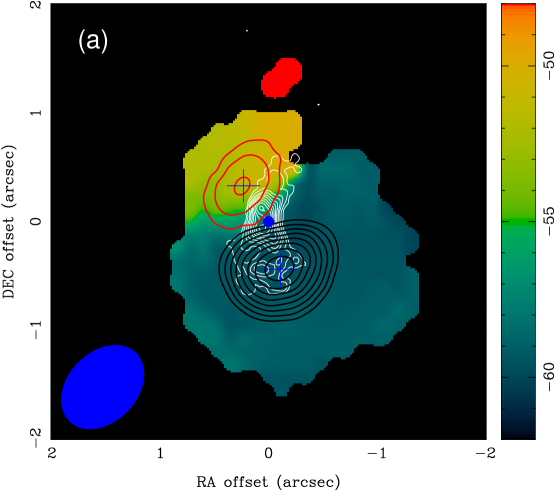
Figure 9.— (a) Same as the Figure 6a, but the red and black contours are for the combined CH₃CN(12-11) $K$=2-5 line. The velocity ranges for integrating ($-54.0$, $-47.0$) km s^-1 and ($-62.5$, $-57.0$) km s^-1 for IRS 1 NE (red) and SW (black), respectively. The contour levels are (0.7, 1.1, 1.4) and (2.8, 3.2, 3.5, 3.9, 4.2, 4.6, 4.9) Jy beam^-1 km s^-1 for IRS 1 NE and SW, respectively. (b) The line profiles of CH₃CN(12-11) $K$=2-5 lines at the positions of IRS 1 SW (solid line) and NE (dashed line). (c) The line profile of CH₃CN(12-11) $K$=2-5 lines integrated over the entire IRS 1 region.

Taking the strong transitions $K$=2-5, with no blending, we combined the visibility data of the four transitions in the LSR-velocity domain to construct the channel maps of CH₃CN(12-11) (Figure 8), which is equivalent to averaging the line intensities from the $K$=2-5 transitions. This spectral line image is referred to as the $K$=2-5 line image, hereafter. Figure 9a shows the integrated line intensity image of IRS 1 SW and NE made from the $K$=2-5 line image, which is in good agreement with that of OCS(19-18) (see Figure 6a). The peak position of IRS 1 SW is ($-0\farcs 11\pm 0\farcs 03$, $-0\farcs 44\pm 0\farcs 03$) offset from IRS 1, based on a Gaussian fitting, while IRS 1 NE is offset by ($0\farcs 23\pm 0\farcs 07$, $0\farcs 33\pm 0\farcs 09$), consistent with OCS(19-18). The centroid velocity distribution made from the CH₃CN(12-11) $K$=2-5 line image is also shown in Figure 9a, showing a similar velocity gradient from SW to NE as that derived from the OCS(19-18) line (see Figure 6a).

Figure 9b shows the spectral profiles made from the $K$=2-5 line image of CH₃CN(12-11) toward the peak positions of IRS 1 SW and NE while Figure 9c is the spectrum integrated over the entire IRS 1 region. Gaussian fitting gives $V_{\rm LSR}=-59.5\pm 0.1$ km s^-1 and $\Delta V_{\rm FWHM}=4.3\pm 0.1$ km s^-1 for IRS 1 SW, and $V_{\rm LSR}=-51.4\pm 0.2$ km s^-1 and $\Delta V_{\rm FWHM}=6.8\pm 0.5$ km s^-1 for IRS 1 NE, respectively. These results are in good agreement with those from OCS(19-18) .

In addition, a weak (more than 3$\sigma$, 1$\sigma$=0.03 Jy beam^-1) absorption of the CH₃CN(12-11) line at $V_{\rm LSR}=-56$ km s^-1 was observed from the $K$=2-5 line image (see Figures 8 and 9c). We will further discuss these possible absorption features.

4.5. Kinetic Temperature of The Hot Molecular Gas

As a symmetric top molecule, CH₃CN is a good probe for determination of the kinetic temperature of the molecular gas. The multiple $K$ transitions for $J\rightarrow J-1$ in a rotational transition of CH₃CN can be observed simultaneously, and their line flux ratios reflect the rotational temperature $T_{\rm rot}$, equivalent to the kinetic temperature $T_{\rm k}$ under LTE condition. Using rotational temperature equilibrium analysis (e.g. Hollis, 1982; Loren et al., 1984; Churchwell et al., 1992; Goldsmith & Langer, 1999; Araya et al., 2005; Furuya et al., 2008), one can determine the kinetic (rotation) temperature $T_{\rm rot}$ and total column density $N$ of the hot molecular gas in an optically thin case by fitting a linear function to the relation between the (logarithmic) column density $N_{JK}$ and the rotational energy $E_{JK}$ at levels ($J,K$) of CH₃CN:

$${\rm ln}\left(\frac{N_{JK}}{g_{JK}}\right)={\rm ln}\left[\frac{N}{Q(T_{\rm rot})}\right]-{\rm ln}\left[\frac{\tau_{J,K}}{1-{\rm e}^{-\tau_{J,K}}}\right]-\frac{E_{JK}}{kT_{\rm rot}},$$ (1)

where $g_{JK}$ is the statistical weight of the level $(J,K)$, $N$ is the total column density, $\displaystyle Q(T_{\rm rot})=3.89T_{\rm rot}^{1.5}/(1-{\rm exp}(-524.8/T_{\rm rot}))^{2}$ is the partition function, and $k$ is Boltzmann constant.

In the case of NGC 7538 IRS 1, some of the $K$ components of CH₃CN(12-11) are obviously optically thick (see Section 4.4). Therefore, we made iterations in fitting the rotation temperature. First, higher $K$ components ($K$=4, 5, 7 and 8 for SW, and $K$=4, 5, and 7 for NE) were assumed to be optically thin and used in the initial fitting with Equation (1) by eliminating the optical-depth term $-{\rm ln}(\tau_{J,K}/(1-{\rm exp}(-\tau_{J,K})))$. The initial fitting gave a rotation temperature $T^{\prime}_{\rm rot}$ and a total column density $N^{\prime}$, with which the corresponding optical depths $\tau^{\prime}_{J,K}$ and optical-depth-correction factors $f^{\prime}_{\tau}(J,K)=\tau_{J,K}/(1-{\rm exp}(-\tau_{J,K}))$ were derived for each $K$ components. In the following iterations, we used $f^{\prime}_{\tau}$ to correct the observed surface column densities $N^{\rm obs}_{JK}$ and added the other $K$ components to the fitting. To avoid the bias caused by the optically thick $K$ components, their weighting in the fitting was inversely proportional to their deviations from the fitting curve of the previous iteration.

The final least-square fitting results are shown in Figure 10, giving rotational temperatures of 260$\pm 30$ K and 260$\pm$60 K for IRS 1 SW and NE, respectively. The derived rotational temperatures are consistent with 297 K reported by Klaassen et al. (2009) and 245 K reported by Qiu et al. (2011). We note that the optically thick components, $K$=0, 1, 2 and 3 for IRS 1 SW and $K$=3 one for NE, significantly deviate from the fitting curve, and have little influence on the fitting results due to their low weighting. The derived optical-depth-correction factors $f_{\tau}(J,K)$, which are based on the fitting results ($N$ and $T_{\rm rot}$), are not adequate to correct the $N_{JK}$ to the fitting curve. The optical depths of the $K$ components used in the initial iterations of the fitting are non negligible.

For the high $K$ components with smaller optical depths, the correction factor $f_{\tau}$ is close to unity and not sensitive to $\tau$, while for the optically thick components, $f_{\tau}$ is almost proportional to $\tau$. An underestimation of the $\tau_{J,K}$ of the high $K$ components will not change the slope of the fit, which is largely determined by these levels. However, the fitted total column density will cause significant underestimations for the $\tau_{J,K}$ and $f_{\tau}(J,K)$ of the optically thick levels, which results in the large deviation from the fit (see Figure 10).

In summary, by fitting the $K$ components of CH₃CN(12-11) lines with small optical depths, we estimated the kinetic temperature of the hot molecular clumps to be $\sim$260 K. The corresponding total column densities for IRS 1 SW and NE, however, might be underestimated by a factor of a few and represent the lower limits. With the derived $T_{\rm rot}$, we can estimate the lower limits of the total column densities $N=1.9\pm 0.5\times 10^{16}$ cm^-2 and $N=3.5\pm 1.5\times 10^{15}$ cm^-2 toward the intensity peaks of SW and NE, respectively. With an abundance of 1$\times$10^-8 for CH₃CN (Qiu et al., 2011, and references therein), these column densities correspond to gas masses of 4 and 0.7 M_⊙ for SW and NE (in one FWHM beam size), respectively.

Figure 10.— The population diagrams with $K$=0, 1, 2, 4, 5, 6, 7, 8 transitions of CH₃CN(12-11) lines for IRS 1 SW, and $K$=0, 1, 2, 4, 5, 6, 7 transitions for NE. The vertical bar marks 1$\sigma$ error. The corresponding measurement of $K$=3 transition is marked with filled square but excluded from the fitting. The straight lines are the best fittings to the data based on linear regression for ${\rm ln}(\frac{N_{JK}}{g_{JK}})=\alpha\frac{E_{JK}}{k}+\beta$, with $\alpha=-0.0038\pm 0.0004$ and $\beta=27.5\pm 0.1$ for IRS 1 SW and $\alpha=-0.0038\pm 0.0012$ and $\beta=25.8\pm 0.4$ for NE.

4.6. ¹³CO(2-1), CO(2-1) & HCN(1-0) toward IRS 1

4.6.1 ¹³CO(2-1) toward IRS 1

The ¹³CO(2-1) line is a good tracer for the gas with a low to intermediate density. We produced a high-velocity ($\delta V=0.5$ km s^-1) and high-angular (0$\farcs$8$\times$0$\farcs$6) resolution image of the ¹³CO(2-1) line to study both the absorption line against the continuum source and the emission line from the molecular gas immediately surrounding IRS 1. Figure 11 shows the channel maps of ¹³CO(2-1), exhibiting a strong absorption between $-60$ to $-53$ km s^-1 toward the 1.3-mm continuum peak and an emission component SW to IRS 1 in the velocity range of ($-63$, $-60$) km s^-1. A similar distribution of ¹³CO(2-1) gas is also shown in Figure 12, the integrated intensity maps of both ¹³CO(2-1) emission and absorption from the velocity range between $-43$ to $-66$ km s^-1. The morphology of the integrated ¹³CO(2-1) emission shows an elongated feature across IRS 1 with a P.A.$\sim$35°. At an offset $\sim$1″  southwest of IRS 1, a blueshifted gas component is also observed from ¹³CO(2-1) emission. In general, both the integrated line flux and the intensity-weighted velocity images derived from the ¹³CO(2-1) line appear to be in good agreement with the results observed from the molecular lines OCS(19-18) and CH₃CN(12-11).

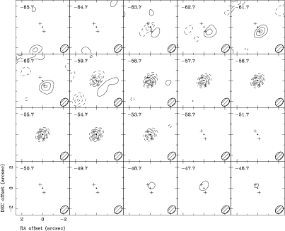
Figure 11.— The channel maps of ¹³CO(2-1). The contours are (…, –4, –3, –2, –1, 1, 2, …)$\times$5$\sigma$, and 1 $\sigma=0.05$ Jy beam^-1. The FWHM beam size is 0$\farcs$8$\times$0$\farcs$6, $\rm P.A.=-44$°. IRS 1 is located at the phase center (indicated by the filled black circle).

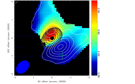
Figure 12.— The images of ¹³CO(2-1) emission (solid white contours) and absorption (dotted contours) constructed by integrating the line intensity from the velocity range between $-43$ to $-66$ km s^-1 with an FWHM beam size 0$\farcs$8$\times$0$\farcs$6 (P.A. $=-45\arcdeg$). The emission contours are 2, 2.5, 3, 3.5, 4 and 4.5 Jy beam^-1 km s^-1. The absorption contours are –2, –2.8, –4, –5.7, –8, –11.3 Jy beam^-1 km s^-1. The intensity-weighted radial velocity (LSR) image (color) was made from the ¹³CO(2-1) emission line in the same velocity range used for the total intensity image of the line emission. The color wedge scales the velocities in the units of km s^-1. The green plus sign indicates the emission peak of the SW 1.3-mm continuum extension.

We made a ¹³CO(2-1) spectrum toward the 1.3-mm emission peak in IRS 1 region and fitted the line profiles with a multiple-Gaussian-component model (see Figure 13a). A narrow ($\Delta V_{\rm FWHM}\sim$ 1 km s^-1) and strong ($\Delta S_{\rm L}=-2.6$ Jy beam^-1) absorption feature at $-59.0$ km s^-1 was observed toward IRS 1, which is best seen in a spectrum made from using the long ($>$100 k$\lambda$) baseline data. The narrow velocity characteristics of this feature suggest that a large fraction of the absorption at the velocity close to the systemic velocity arises from the absorption by the cold gas in the molecular envelope located in front of the continuum source IRS 1. The absorption peak velocity in ¹³CO(2-1) verifies that the systemic velocity of IRS 1 is very close (within 0.5 km s^-1) to $V_{\rm sys}=-59.0$ km s^-1 as observed in other molecular lines. Given $\Delta S_{\rm L}=-2.6$ Jy beam^-1 and $S_{\rm C}=3.25$ Jy beam^-1 the peak optical depth of the ¹³CO(2-1) line can be determined for the main absorption feature near the systemic velocity using Equation (1) of Qin et al. (2008), $\tau_{\rm L}=-{\rm ln}\left(1+\Delta S_{\rm L}/S_{\rm C}\right)=1.6$.

Two more absorption components are seen at $-57.0$ and $-54.0$ km s^-1, which are likely due to infall toward the central source in IRS 1. For these two absorption features, the equivalent total line width is $\sim$5 km s^-1, which is consistent with the main absorption feature in the inverse P-Cygni profile suggested from the lower-angular resolution observations of the HCO⁺(1-0) line (Corder, 2008; Sandell et al., 2009). A weak (0.5 Jy beam^-1), and broad ($\Delta V_{\rm FWHM}=5.5$ km s^-1) emission at velocity $-63.0$ km s^-1 was also detected, corresponding to the blueshifted emission in the inverse P-Cygni profile from lower angular resolution observations.

Two additional significant spectral features in ¹³CO(2-1) were also detected: a blueshifted absorption component ($\Delta S_{\rm L}=-0.5$ Jy beam^-1, $\Delta V_{\rm FWHM}=1.3$ km s^-1) at $V_{\rm LSR}=-63.8$ km s^-1 and a redshifted emission component ($\Delta S_{\rm L}=0.45$ Jy beam^-1, $\Delta V_{\rm FWHM}=2.5$ km s^-1) at $V_{\rm LSR}=-48.0$ km s^-1. The blueshifted absorption component is probably due to the foreground outflow gas, for which we find $\tau_{\rm L}=-{\rm ln}\left(1+\Delta S_{\rm L}/S_{\rm C}\right)\approx 0.17$. While the redshifted emission at $V_{\rm LSR}=-48.0$ km s^-1 could also be due to outflow, it more likely traces a background cloud emission at the same radial velocity, as indicated by lower-resolution studies on the general gas distribution in the NGC 7538 region (Sandell 2013, private communications).

To estimate the column density of the observed ¹³CO gas, a reasonable excitation temperature $T_{\rm ex}$ is needed. The absorption feature of ¹³CO (2-1) is seen only in the central 1$\farcs$5 region in projection. If the ¹³CO gas is all within the central 1$\farcs$5, and co-exists with the hot molecular gas, then a high $T_{\rm ex}$ of $\sim$200 K is appropriate. However, the lack of the ¹³CO absorption outside the 1$\farcs$5 region might be simply due to the absence of an emission background. In this case, the ¹³CO absorption arises from gas along the line of sight, and a lower excitation temperature should be considered. Sandell & Sievers (2004) derived a $T_{\rm d}$ of 75 K from fitting the dust emission in a $\sim$11$\farcs$5$\times$10$\farcs$6 region around IRS 1, constrained by the sub-millimeter luminosity of IRS 1. We calculated the total ¹³CO column density with both the high $T_{\rm ex}=200$ K (upper limit) and low $T_{\rm ex}=75$ K (lower limit) for each velocity component of ¹³CO (2-1) and listed the results in Table 5.

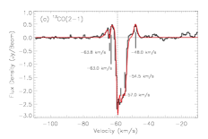
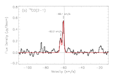
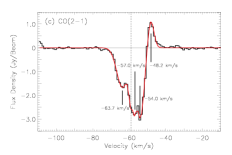
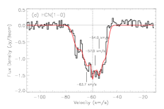
Figure 13.— (a), (c) and (d): the ¹³CO(2-1), CO(2-1) and HCN(1-0) spectra toward IRS 1, respectively. (b) the ¹³CO(2-1) spectrum toward the position of the 1.3-mm SW extension. In all the figures, the dashed vertical lines mark V${}_{\rm sys}=-59.0$ km s^-1, and the red curves are the multiple-Gaussian fitting to the line profiles. The parameters for each of the kinematic components from the fitting are summarized in Table 5.

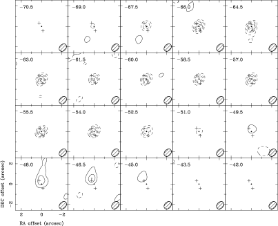
Figure 14.— The channel maps of CO(2-1). The contours are (…, –4, –3, –2, –1, 1, 2, 3, 4…)$\times$5$\sigma$, and 1 $\sigma=0.1$ Jy beam^-1. The FWHM beam size is 0$\farcs$8$\times$0$\farcs$6, $\rm P.A.=-42$°. IRS 1 is located at the phase center (indicated by the filled black circle).

We also extracted a ¹³CO(2-1) spectrum toward the “SW tail” structure observed in the 1.3-mm continuum (Figure 13b). Toward the position of the SW extension in 1.3-mm continuum, a narrow ($\Delta V_{\rm FWHM}\approx 1.8$ km s^-1) emission feature at $-60.1$ km s^-1 with $\Delta S_{\rm L}=0.6$ Jy beam^-1 is seen close to $V_{\rm sys}$, which seems to be affected by the contamination from the spectrum from IRS 1 and has a skewed line profile. In addition, a narrow, weaker emission feature ($\Delta V_{\rm FWHM}\sim 2.1$ km s^-1, $\Delta S_{\rm L}=0.2$ Jy beam^-1) at $-63.2$ km s^-1 is detected which could be associated with low-velocity outflow gas.

4.6.2 CO(2-1) toward IRS 1

We made channel maps of CO(2-1) (Figure 14), showing a wide absorption toward IRS 1 from $-69$ to $-52$ km s^-1. Multiple spectral components are included in this wide absorption, which are best seen in the CO(2-1) spectra toward the 1.3-mm emission peak in IRS 1 (Figure 13c) and the Gaussian fitting. Absorption features at velocities $-63.7$, $-59.0$, $-57.0$ and $-54.0$ km s^-1, an emission feature at $-48.2$ km s^-1, and the fitting results are summarized in Table 5. The fitting results are in good agreement with ¹³CO(2-1) except for the absorption feature at $-63.7$ km s^-1 which is much deeper ($\Delta S_{\rm L}=-1.7$ Jy) and much broader ($\Delta V_{\rm FWHM}=7$ km s^-1) than its ¹³CO(2-1) counterpart. The CO(2-1) counterpart corresponding to the blueshifted emission observed in ¹³CO(2-1) at $-63.0$ km s^-1 was not detected, which might be diluted by the strong and broad absorption feature at $-63.7$ km s^-1. The wide blueshifted CO(2-1) absorption is likely due to foreground outflow gas. The optical depths of the CO(2-1) features are determined with $\tau_{\rm L}=-{\rm ln}(1-\Delta S_{\rm L}/S_{\rm C})$, showing the large optical depths ($\sim 3$) of the CO(2-1) components that are associated with the redshifted absorption gas, and suggesting that the infalling CO(2-1) gas is optically thick.

4.6.3 HCN(1-0) Hyperfine Lines & Absorption Profile

The $J$=1-0 transition of HCN has three hyperfine lines ($F$=0-1, 1-1 and 2-1) with optical depths in the ratio 1:3:5 under LTE. The strongest line $F$=2-1 has $\nu_{0}=88.6318$ GHz. The velocity separations of $F$=1-1 and $F$=0-1 with respect to $F$=2-1 are +4.84 and $-$7.08 km s^-1, respectively. We made multiple Gaussian fits to the four kinematic components in absorption identified in CO(2-1) to the HCN(1-0) absorption profile (Figure 13d). For each kinematic component, we used the three hyperfine lines of the HCN(1-0) transition in the initial fitting. In the fits, the intensity ratio of each hyperfine line was fixed assuming LTE, and the FWHM line widths for the hyperfine components were kept to be the same for each kinematic component. The three parameters $\Delta S_{\rm L}$, $V_{\rm LSR}$ and $\Delta V_{\rm FWHM}$ for the main hyperfine lines ($F$=2-1) are determined from the best fitting. However, the hyperfine lines $F$=0-1 and $F$=1-1 in the high blueshifted and high redshifted ends of the absorption profile require high intensities that do not fit to their corresponding LTE ratio. The high-velocity HCN line features might be non-LTE. Alternatively, the broadening of the HCN(1-0) absorption profile might be caused by high-velocity gas components which are associated with shocked or compressed gas and traced by the HCN emission (e.g. Shi et al., 2010). The absorptions caused by these high-velocity gas components might be insignificant in CO(2-1) due to the mitigation of the emission of the CO(2-1) outflow. Table 5 summarizes the fitting results.

5. Discussion

5.1. A Massive Ionizing Star in the HC H II region IRS 1

IRS 1 is a HC H II region associated with a newborn star. At the high-angular resolution ($\sim$0$\farcs$3) in the CARMA observations, the surrounding dust emission has been resolved out. Fitting the continuum fluxes of IRS 1 at multiple wavelengths indicates that even at 1.3-mm the free-free emission still dominates the continuum emission (Sandell et al., 2009). If we assume optically thin emission and neglect the contribution of the thermal dust emission, a Lyman continuum flux $N_{\rm Lym}$ can be estimated from the 1.3 mm flux density ($S_{\rm C}=3.8$ Jy at $\nu=224$ GHz) of IRS 1 with the equation below of a recombination coefficient of $\alpha_{\rm B}=2.58\times 10^{-13}$ cm^-3 s^-1 in case B and electron temperature of $T_{\rm e}=1\times 10^{4}$ K (Hummer & Seaton, 1963),

$$N_{\rm Lym} = 7.6\times 10^{46}\,{\rm phot\,s^{-1}}\,\alpha^{-1}(\nu,T_{\rm e})\times$$ (2)

$$\left(\frac{T_{\rm e}}{10^{4}\,K}\right)^{0.35}\left(\frac{\nu}{\rm GHz}\right)^{0.1}\left(\frac{S_{\rm C}}{\rm Jy}\right)\left(\frac{D}{\rm kpc}\right)^{2},$$

where the correction factor for power-law approximation $\alpha(\nu,T_{\rm e})=0.85$ for $T_{\rm e}=10,000$ K and $\nu=224$ GHz (Mezger & Henderson, 1967). For $D=2.65$ kpc, we have $N_{\rm Lym}=4.1\times 10^{48}$ phot s^-1. At 224 GHz, our observations might not be sensitive enough to reveal the extended structures of the ionized outflow as the VLA observations shown (see Figure 2). However, with Equation (2) and the U-band measurement (60 mJy, see Sandell et al., 2009), it suggests that only $\sim$2$\times$10⁴⁶ photo s^-1 was contributed by the extended structure, less than 1% of the 224-GHz results.

However, a few caveats need to be kept in mind for the above estimate. First, most of the free-free emission in the unresolved central region ($\leq$0$\farcs$1) is actually optically thick, resulting in underestimation of the uv photon flux from the YSO in IRS 1. Second, the contribution of dust thermal emission might not be negligible. If we extrapolate the total flux density fit for IRS 1 from the spectrum between 4.8 and 43.4 GHz (Sandell et al., 2009) to 224 GHz, a total flux of $\sim$2.6 Jy from free-free emission is predicted, implying that dust thermal emission might contribute $\sim$30 percent of the total flux density. In addition, ionization is not only due to the UV photons from the stellar photosphere but also caused by the heating in the accretion process. For low-mass pre-main-sequence stars (classical T Tauri stars, CTTSs), the shock front due to accretion will produce hot plasma with a temperature of a few times of 10⁶ K and yield significant emission in the soft X-ray band (Argiroffi et al., 2012). It is possible that in the case of high-mass YSOs with ongoing accretion similar processes also occur, and produce high-energy photons which will ionize surrounding molecular gas. Unfortunately, currently there is no detailed quantitative model on how much Lyman continuum flux the accretion process can contribute for the high-mass YSOs. However, we believe that the uv photons from the stellar photospheres of the YSOs are the dominating source for photoionization.

Neglecting all the factors described above, this Lyman continuum flux of $\sim$4.1$\times$10⁴⁸ phot s^-1 is equivalent to the flux from a single star of O8-O9.5 in the main sequence (Vacca et al., 1996; Martins et al., 2005), which is required to maintain the ionization of the HC H II region IRS 1 alone. Taking account of the possible overestimation of 30% due to dust thermal emission will not change the derived spectral type. Considering the fact that we might significantly underestimated the continuum flux due to optical depth effects, the assessment for the spectral type of the ionizing star is also consistent with the suggestions of an O6/7 star estimated previously (e.g. Willner, 1976; Akabane & Kuno, 2005) if the turn-over frequency for the free-free emission from the HC HII region is significantly higher than 230 GHz ($\lambda\sim$1.3 mm). Then, the massive ionizing star should be the primary energy source, responsible for ionizing the HC H II region and driving the energetic ionized outflow via the overwhelming radiative pressure.

5.2. Infalling Gas

As suggested by Corder (2008), Sandell et al. (2009) and Beuther et al. (2012), an on-going accretion might be taking place in the IRS 1 system. From the ¹³CO(2-1) absorption in front of the IRS 1 core, the total column density of molecular gas is 2.0$\times 10^{24}$ cm^-2 using [CO]/[H₂]=10^-4, [¹³CO]/[CO]=1/60 and a high $T_{\rm ex}$=200 K (see Table 5). If the molecular gas is spherically and evenly distributed within a radius of 1900 AU (equivalent to the 0$\farcs$7 FWHM beam size of the CARMA 1.3-mm observations), this column density implies that about 5 M_⊙ in the surrounding region is available for accretion onto IRS 1. On the other hand, if we adopt a large-scale distribution of the ¹³CO gas (the lower column density of 8$\times$10²³ cm^-2 corresponding to the lower $T_{\rm ex}=75$ K needs to be considered), the mass of the molecular gas associated with IRS 1 would be larger since its value is proportional to the square of radius.

The inverse P-Cygni profile revealed from the observations of HCO⁺(1-0) by Corder (2008) & Sandell et al. (2009) suggests that the infall likely occurs within the beam size of 4$\farcs$5, or the inner region with a size of 0.06 pc. Our sub-arcsec resolution observations of HCN(1-0), CO(2-1) and ¹³CO(2-1) lines toward IRS 1 agree with the previous results.

Absorption features are also detected in OCS(19-18) and $K$=2-5 components of CH₃CN(12-11) (see Sections 4.3 and 4.4) in the velocity range bettwen $-56.5$ to $-53.0$ km s^-1, corresponding to the absorption features at $-57.0$ and $-54.0$ km s^-1 in HCN(1-0), CO(2-1) and ¹³CO(2-1). These absorptions probably arise in the infalling gas, revealing the hot dense gas in the accretion flow. The hot molecular gas is more redshifted than the corresponding HCN(1-0) and CO absorptions, perhaps tracing an accelerating infall closer to IRS 1.

The redshifted ¹³CO(2-1) absorption against the continuum radiation from IRS 1 clearly shows evidence for ongoing gas infall. From the optical depth of the infalling gas determined from the relatively optically thin line ¹³CO(2-1), as well as the excitation temperature determined from the CH₃CN population diagram, we can estimate the infall rate $\displaystyle dM/dt=4\pi r^{2}m_{\rm H}\mu n_{\rm H}V_{\rm in}$, at an infall radius $r$, where the mean molecular weight $\mu=2.35$ and density of the accretion materials $n_{\rm H}=N_{\rm H}/r$. Thus, the infall rate is a function of the measurable quantities,

$$\frac{dM}{dt} = 2.8\times 10^{-4}\,{\rm M}_{\odot}\,{\rm yr}^{-1}\left[\frac{\theta_{\rm in}}{\rm arcsec}\right]\left[\frac{D}{\rm kpc}\right]$$ (3)

$$\left[\frac{N_{\rm H}}{\rm 10^{24}\,{\rm cm}^{-2}}\right]\left[\frac{\Delta V_{\rm in}}{\rm km~{}s^{-1}}\right],$$

where the angular size of the infall region $\theta_{\rm in}$ is approximately of the geometric mean of the telescope beam $\theta_{\rm B}=0\farcs 7$.

The two redshifted absorption components at $-54.5$ and $-57.0$ km s^-1 in ¹³CO(2-1) give H₂ column densities ($N_{\rm H,red}$) of 9$\times$10²³ and 1$\times$10²⁴ cm^-2, respectively. If we take the velocity displacements of the two absorption features from the systemic velocity as their corresponding infall velocity ($V_{\rm in}\approx\Delta V=V_{\rm LSR}-V_{\rm sys}$), an infall rate of 3$\times$10^-3 $\rm M_{\odot}$ yr^-1 can be inferred based on equation (3) for the IRS 1 region, higher than the value derived by previous study (Corder, 2008; Sandell et al., 2009), lower than that of Beuther et al. (2012) and agree with that of Qiu et al. (2011). In addition, as discussed in Section 4.6.1, we might underestimate the size of the infalling region, and thus overestimate the characteristic excitation temperature of the ¹³CO gas in this region. However, since in equation (3) the column density $N_{\rm H}$ is proportional to excitation temperature, we expect that the different approach (larger infalling region, low characteristic T_ex) would not significantly change the derived infall rate.

The infall rate can also be estimated from the HCN(1-0) results despite larger uncertainty in the the line profile fitting, and the poor determination of the abundance. On the basis of Rolfs & Wilson (2004), the column density of HCN can be derived by:

$$N({\rm HCN}) = 5.41\times 10^{11}{\rm cm}^{-2}\frac{T_{\rm ex}\int\tau_{v}{\rm d}v}{1-{\rm exp}(-4.25/T_{\rm ex})}$$ (4)

With $T_{\rm ex}=200$ K, the two redshifted absorption HCN(1-0) components at $-54.0$ and $-57.0$ km s^-1 give HCN column densities of $N_{\rm HCN}=5\times 10^{16}$ and $N_{\rm HCN}=1\times 10^{16}$ cm^-2, respectively. A recent study reported a H¹³CN abundance of $\sim$2$\times$10^-10 in active star formation regions (Zinchenko et al., 2009), so we estimate a total H₂ column density $N(\rm H_{2})=5\times 10^{24}$ cm^-2 with ${\rm[H^{13}CN]/[HCN]}=1/60$, which corresponds to an infall rate of 1$\times$10^-2 $\rm M_{\odot}$ yr^-1, triple of the value derived from ¹³CO(2-1). Although the infall rates derived from ¹³CO (2-1) and HCN(1-0) are relatively high, they are still in the typical range of 10^-4 to 10^-2 M_☉ yr^-1 for embedded high-mass cores (Wu et al., 2009, and the references therein).

We can compare the derived infall rates with an ideal free-fall case. With an enclosed mass of 30 M_☉ (including the masses of both gas and the central star) at a radius $r=$0$\farcs$7, the free-fall infall velocity $V_{\rm in,ff}$ is about 5.5 km s^-1, corresponding to a free-fall infall rate of 5$\times$10^-3 M_☉ yr^-1 from the ¹³CO(2-1) results. This value agrees with 3$\times$10^-3 M_☉ yr^-1, calculated from the velocity displacements of the redshifted ¹³CO (2-1) absorption features, indicating that gas is falling into IRS 1 rapidly.

In addition to the redshifted absorption velocity components, we see a blueshifted absorption at $V_{\rm lsr}=-63.8$ km s^-1 in ¹³CO(2-1) or $V_{\rm lsr}=-63.7$ km s^-1 in CO(2-1) and HCN(1-0). Since the optical depths of the blueshifted absorption are significantly lower than the redshifted ones, and no other observations have suggested a cloud component in NGC 7538 region at this radial velocity which is only seen toward IRS 1, we believe that the absorption line components at $-63.7$ or $-63.8$ km s^-1 arise from the blueshifted outflow gas between IRS 1 and the observer.

5.3. The Nature of Hot Molecular Clumps & Dynamics in NGC 7538 IRS 1

The kinematics observed from IRS 1 SW and NE in the central 2$\arcsec$, from OCS(19-18), CH₃CN(12-11) and ¹³CO(2-1) show a velocity gradient in P.A.$\sim$43$\arcdeg$. The three molecular species observed in this paper are in good agreement with the results from the ¹³CO(1-0) emission (Scoville et al., 1986) and ¹⁵NH₃ masers (Gaume et al., 1991) observations.

The observed high excitation temperatures and velocities of the hot molecular components in the circumstellar region of IRS 1 provide clues for understanding the IRS 1 system. Infrared radiation from IRS 1 supplies the primary heating in the central 1-2″, ($\sim$5,000 AU). The ionized emission observed with the VLA in the inner $<2\arcsec$(Campbell, 1984; Gaume et al., 1995; Sandell et al., 2009) is suggested to be a hot ionized wind with a velocity up to 300 km s^-1 which is partially confined and collimated by the molecular material surrounding IRS 1 (Gaume et al., 1995). The hot molecular components (see Figure 6a and 9a) are located NE of the ionized core, and SW of the southern lobe of the ionized outflow. These two locations are close to the path of the ionized outflow, suggesting that the molecular gas may be heated by the interaction between the ionized outflow and accreting gas.

A large accretion flow with a rate of 3-10$\times 10^{-3}$ M_⊙ y^-1 continues to accumulate matter into the circumstellar region around IRS 1 (see Section 5.2). Confronting the overwhelming pressure from the accretion flow, the HC H II region surrounding the O star must be highly confined, and difficult to expand to form a larger size H II region. The excess angular momentum in the infalling gas must be transported out. The outflow provides a mechanism for transferring the angular momentum of the infalling gas.

The large-scale CO(2-1), ¹³CO(1-0) and HCO⁺(1-0) images from CARMA, SMA and single-dish observations suggest a bipolar outflow in a north-south direction with an opening angle greater than $\sim$90°(Sandell et al., 2012). The interaction between this wide-angle molecular outflow and the envelope of ambient molecular gas around IRS 1 might excite the observed hot molecular components, redshifted to the NE, and blueshifted to the SW. The density of the environment is much higher to the south of IRS 1; thus the molecular emission from IRS 1 SW is stronger, and the ionized outflow in this direction is highly confined.

The redshifted radial velocity of IRS 1 NE could also be due to rotation of the wide-angle outflow around its axis. An ionized outflow which rotates around its axis could entrain the adjacent molecular gas, and consequently, the impact of the ionized outflow on the circumstellar gas could produce highly-excited molecular species at the positions of IRS 1 NE and SW.

The ambient density is higher to the south and SW of IRS 1, so the entrainment of the ionized jet is not significant. To the north of IRS 1, the density is lower, and the ionized outflow can penetrate and produce significant redshifted movement of the entrained gas NE of IRS 1. We can roughly estimate the angular momentum of the NE component to be 3.6$\times$10¹⁷ M_☉ m² s^-1 by assuming a mass $M_{\rm NE}=1$ M_☉ (see Section 4.5), rotation velocity $v_{\rm NE}=8$ km s^-1, and radius $r_{\rm NE}=300$ AU ($\Delta\alpha=0\farcs 11$, see Table 4). The angular momentum input to IRS 1 is about 5.7$\times$10¹⁵ M_☉ m² s^-1 yr^-1 with an infall rate of 5$\times$10^-3 M_☉ yr^-1, a radius of 1900 AU ($\sim$0$\farcs$7) and an enclosed mass of 30 M_☉. Therefore, it is plausible that the ionized outflow could cause the observed redshifted movement of the component NE in the lifetime of the accretion process.

6. Conclusion

Using sub-arcsec resolution observations at 1.3 and 3.4 mm with SMA and CARMA, we analyzed the molecular lines and continuum emission from NGC 7538 IRS 1 to investigate the dynamic processes related to the star-forming activities in this region. With an image convolved to 0$\farcs$1 from CARMA B-array observation at 1.3 mm, the primary continuum source IRS 1, an HC H II region, was resolved into two components, an unresolved compact core with a linear size $<270$ AU and a north-south extended lobe of the ionized outflow in agreement with the predicted extrapolation of a power-law dependence made by Sandell et al. (2009). Both the SMA and CARMA show extended dust continuum emission to the SW of IRS 1, which might indicate a reservoir of molecular gas.

The molecular lines OCS(19-18), CH₃CN(12-11) and ¹³CO(2-1), show that dense molecular gas is primarily distributed southwest to northeast across IRS 1 with an angular size of $\sim$2″$\times$1″. The locations and velocities of the molecular clumps suggest that they might be heated by interaction between the ionized outflow from IRS 1 and the adjacent molecular gas in a rotating wide-angle outflow in a N-S direction from IRS 1.

From high-resolution (0$\farcs$8$\times$0$\farcs$6) observations of ¹³CO(2-1), CO(2-1) and HCN(1-0), we fitted multiple Gaussian velocity components to the spectra toward the continuum sources in IRS 1. We found that the significant molecular lines in absorption are redshifted with respect to the systemic velocity toward IRS 1, suggesting that a large amount of material surrounding the region is infalling toward IRS 1. An infall rate of $\sim$3-10$\times$10^-3 M_☉ y^-1 was inferred from ¹³CO(2-1) and HCN(1-0) lines.

Table 1Log of Observation, uv data and images

VISIBILITY DATA SETS
Obs. Date	Obs. pointing		Array Conf.		Calibrators
	$\alpha_{\rm J2000}$	$\delta_{\rm J2000}$		phase	bpass	flux
SMA at 1.3 mm
2008-05-05	23:13:45.362	61:28:10.49	VEX	J2202+422	3C454.3	Vesta
2005-09-11	23:13:45.300	61:28:10.00	EXT	J0102+584	3C454.3	Ceres
				J2202+422	Neptune
CARMA at 1.3 mm
2010-01-04	23:13:45.600	61:28:11.00	B-array	J0102+584	3C454.3	Uranus, MWC349
2010-01-05	23:13:45.600	61:28:11.00	B-array	J0102+584	3C454.3	Neptune
2010-11-10	23:13:45.600	61:28:11.00	C-array	J0102+584	3C454.3	Uranus
2009-11-23	23:13:45.600	61:28:11.00	C-array	J0102+584	3C84	Uranus
2009-11-27	23:13:45.600	61:28:11.00	C-array	J0102+584	3C454.3	MWC349
2010-11-29	23:13:45.600	61:28:11.00	C-array	J0102+584	3C454.3	Neptune
2007-03-15	23:13:45.600	61:28:11.00	C-array	J0102+584	3C454.3	MWC349
2010-08-24	23:13:45.600	61:28:11.00	D-array	J0102+584	3C454.3	Uranus
2009-08-07	23:13:45.600	61:28:11.00	D-array	J0102+584	3C454.3	Neptune
2010-08-27	23:13:45.600	61:28:11.00	D-array	J0102+584	3C454.3	Neptune
2010-08-27	23:13:45.600	61:28:11.00	D-array	J0102+584	3C454.3	Neptune
2010-09-08	23:13:45.600	61:28:11.00	D-array	J0102+584	3C454.3	Uranus
2010-07-05	23:13:45.600	61:28:11.00	E-array	J0102+584	3C454.3	MWC349
2010-07-07	23:13:45.600	61:28:11.00	E-array	J0102+584	3C454.3	MWC349
2010-07-08	23:13:45.600	61:28:11.00	E-array	J0102+584	3C454.3	URANUS
CARMA at 3.4 mm
2010-12-29	23:13:45.298	61:28:10.00	B-array	J0102+584	3C454.3	Uranus
CONTINUUM & LINE IMAGES
Mode	FWHM beam	rms	BW	$\delta V$	$V_{\rm LSR}$-ranges	uv datasets
	″$\times$″(°)	mJy b-1 (ch-1)	GHz	km s-1	km s-1
SMA
Continuum 1.3 mm	0.8$\times$0.6 (–45)	4	4	$\cdots$	$\cdots$	VEX + EXT
Line OCS(19-18)	0.8$\times$0.6 (–45)	60	$\cdots$	0.5	–85 to –35	VEX + EXT
Lines CH3CN(12-11)	0.8$\times$0.6 (–45)	60	$\cdots$	0.5	–85 to –35	VEX + EXT
Line 13CO (2-1)	0.8$\times$0.6 (–45)	50	$\cdots$	0.5	–110 to –10	VEX + EXT
Line 12CO (2-1)	0.8$\times$0.6 (–45)	60	$\cdots$	1	–160 to +40	VEX + EXT
CARMA
Continuum 1.3 mm	0.78$\times$0.64 (–84)	2.5	2-3	$\cdots$	$\cdots$	B+C+D+E-array
Continuum 1.3 mm	0.34$\times$0.27 (–83)	10	2	$\cdots$	$\cdots$	B-array
Continuum 3.4 mm	0.8$\times$0.7 (–68)	7	0.064	$\cdots$	$\cdots$	B-array
Line HCN(1-0)	0.8$\times$0.7 (–68)	33	$\cdots$	1.65	–220 to –11	B-array

Table 2Results from continuum observations at 1.3 & 3.4 mm

Source	$S_{\rm p}$	$S_{\rm t}$	$\Delta\alpha$, $\Delta\delta$	$\Delta\theta_{\rm M}\times\Delta\theta_{\rm m}$ (P.A.)
	(Jy beam-1)	(Jy)	(″, ″)	(″$\times$″(°))
SMA Results
SMA 1.3 mm
IRS 1	3.3$\pm$0.3	3.5$\pm$0.4	0.0$\pm$0.1, 0.0$\pm$0.1	unresolv
SW Extenstion	$0.12\pm$0.02	$0.25\pm$0.04	–0.5$\pm$0.1, –0.9$\pm$0.1	1.0$\times$0.6 (22)
CARMA 1.3 mm
IRS 1-Peak	1.0$\pm$0.1	1.0$\pm$0.1	–0.08$\pm$0.02, –0.07$\pm$0.02	unresolv
IRS 1-Lobe	0.22$\pm$0.02	2.8$\pm$0.3	–0.08$\pm$0.01, –0.09$\pm$0.01	0.42$\times$0.28 (–2)
IRS 1-total	$\cdots$	3.8$\pm$0.4	$\cdots$	$\cdots$
CARMA 3.4 mm
IRS 1	0.93$\pm$0.10	0.93$\pm$0.10	$0.0\pm$0.1, $0.0\pm$0.1	unresolv

Note. — The reference position is R.A. (J2000) = 23^h13^m45.^s37, Dec. (J2000) = 61$\arcdeg$28$\arcmin$10$\farcs$43

Table 3Fitting of the high transition lines at 0.86 mm

Transition	$\nu$	$\Delta S_{\rm L}$	$V_{\rm LSR}$	$\Delta$$V_{\rm FWHM}$
	(GHz)	(Jy beam-1)	(km s-1)	(km s-1)
CH3OH(12,1,11-12,0,12)	336.865	27.8$\pm$0.4	–58.7$\pm$0.1	4.8$\pm$0.2
13CH3OH(12,1,11-12,0,12)	335.560	6.2$\pm$0.2	–58.5$\pm$0.1	3.1$\pm$0.2
13CH3OH(14,1,13-14,0,14)	347.188	4.9$\pm$0.2	–58.6$\pm$0.1	3.4$\pm$0.2

Table 4Properties of Hot Molecular Components in IRS 1

Transition	$\nu$	$\Delta\alpha,\Delta\delta$	$\Delta S_{\rm L}$	$V_{\rm LSR}$	$\Delta V_{\rm FWHM}$	$\displaystyle\int T_{\rm B}{\rm dv}{\rm(peak)}$	$N^{\rm obs}_{JK}$	$N^{\rm corr}_{JK}$	$g_{JK}$	$E_{JK}/k$
	(GHz)	(″)	(Jy b-1)	(km s-1)	(km s-1)	(K km s-1)	(1013 cm-2)			(K)
IRS 1 SW
CH3CN
120-110	220.747	–0.16$\pm$0.04, –0.44$\pm$0.03	1.4$\pm$0.1	–59.3$\pm$0.1	4.4$\pm$0.2	282$\pm$22	2.9$\pm$0.2	$\cdots$	100	68
121-111	220.743	–0.15$\pm$0.06, –0.45$\pm$0.05	1.4$\pm$0.1	–59.2$\pm$0.1	3.9$\pm$0.3	258$\pm$21	2.7$\pm$0.2	$\cdots$	100	76
122-112	220.730	–0.11$\pm$0.04, –0.45$\pm$0.03	1.4$\pm$0.1	–59.6$\pm$0.1	4.2$\pm$0.2	260$\pm$24	2.8$\pm$0.3	$\cdots$	100	97
123-113	220.709	–0.21$\pm$0.04, –0.48$\pm$0.03	1.4$\pm$0.1	–59.6$\pm$0.1	4.3$\pm$0.1	282$\pm$18	2.8$\pm$0.2	$\cdots$	200	133
124-114	220.679	–0.07$\pm$0.03, –0.43$\pm$0.03	1.2$\pm$0.1	–59.5$\pm$0.1	4.2$\pm$0.2	249$\pm$23	2.8$\pm$0.3	3.3$\pm$0.3	100	183
125-115	220.641	–0.04$\pm$0.04, –0.41$\pm$0.03	0.9$\pm$0.1	–59.5$\pm$0.1	4.6$\pm$0.3	201$\pm$26	2.5$\pm$0.3	2.8$\pm$0.4	100	247
126-116	220.594	–0.01$\pm$0.04, –0.30$\pm$0.03	0.9$\pm$0.1	–59.5$\pm$0.1	4.5$\pm$0.2	205$\pm$20	2.8$\pm$0.3	3.2$\pm$0.3	200	326
127-117	220.539	+0.08$\pm$0.09, –0.25$\pm$0.08	0.5$\pm$0.1	–59.5$\pm$0.2	4.1$\pm$0.4	97$\pm$23	1.5$\pm$0.4	1.5$\pm$0.4	100	419
128-118	220.476	+0.06$\pm$0.10, –0.45$\pm$0.12	0.3$\pm$0.1	–59.3$\pm$0.2	3.4$\pm$0.4	54$\pm$12	1.0$\pm$0.2	1.0$\pm$0.2	100	526
($K$=2-5)		–0.11$\pm$0.03, –0.44$\pm$0.02	1.2$\pm$0.1	–59.5$\pm$0.1	4.3$\pm$0.1	250$\pm$16	$\cdots$	$\cdots$	$\cdots$	$\cdots$
OCS
19-18	231.061	–0.13$\pm$0.03, –0.41$\pm$0.03	1.3$\pm$0.1	–59.5$\pm$0.1	4.4$\pm$0.1	267$\pm$15	$\cdots$	$\cdots$	$\cdots$	$\cdots$
IRS 1 NE
CH3CN
120-110	220.747	+0.39$\pm$0.15, +0.26$\pm$0.25	0.6$\pm$0.1	–52.0$\pm$0.2	5.4$\pm$0.5	164$\pm$22	1.4$\pm$0.2	1.5$\pm$0.2	100	69
121-111	220.743	+0.21$\pm$0.03, +0.33$\pm$0.03	0.5$\pm$0.1	–51.4$\pm$0.4	5.4$\pm$0.5	138$\pm$24	1.4$\pm$0.2	1.5$\pm$0.3	100	76
122-112	220.730	+0.23$\pm$0.04, +0.36$\pm$0.06	0.4$\pm$0.1	–51.4$\pm$0.3	6.0$\pm$0.7	109$\pm$23	1.2$\pm$0.2	1.2$\pm$0.3	100	97
123-113	220.709	+0.26$\pm$0.06, +0.28$\pm$0.07	0.3$\pm$0.1	–51.0$\pm$0.3	5.7$\pm$0.6	96$\pm$14	1.1$\pm$0.2	$\cdots$	200	133
124-114	220.679	+0.14$\pm$0.15, +0.35$\pm$0.16	0.3$\pm$0.1	–51.3$\pm$0.3	4.4$\pm$0.7	61$\pm$18	0.7$\pm$0.2	0.7$\pm$0.2	100	183
125-115	220.641	+0.31$\pm$0.06, +0.12$\pm$0.08	0.3$\pm$0.1	–52.0$\pm$0.5	4.1$\pm$0.6	49$\pm$15	0.6$\pm$0.2	0.6$\pm$0.2	100	247
126-116	220.594	+0.24$\pm$0.06, +0.27$\pm$0.08	0.4$\pm$0.1	–50.8$\pm$0.2	3.4$\pm$0.2	60$\pm$10	0.8$\pm$0.1	0.9$\pm$0.2	200	326
127-117	220.539	+0.42$\pm$0.15, +0.06$\pm$0.16	0.2$\pm$0.1	–51.1$\pm$0.3	2.8$\pm$0.5	26$\pm$11	0.4$\pm$0.2	0.4$\pm$0.2	100	419
($K$=2-5)		+0.23$\pm$0.04, +0.33$\pm$0.04	0.3$\pm$0.1	–51.4$\pm$0.2	6.8$\pm$0.5	103$\pm$14	$\cdots$	$\cdots$	$\cdots$	$\cdots$
OCS
19-18	231.061	+0.25$\pm$0.03, +0.35$\pm$0.02	0.5$\pm$0.1	–51.5$\pm$0.3	7.2$\pm$0.6	180$\pm$30	$\cdots$	$\cdots$	$\cdots$	$\cdots$

Note. — The reference position is R.A. (J2000) = 23^h13^m45.^s37, Dec. (J2000) = 61$\arcdeg$28$\arcmin$10$\farcs$43

Table 5¹³CO(2-1), CO(2-1) and HCN(1-0) toward IRS 1

Source	$\Delta\alpha$, $\Delta\delta$	$\Delta S_{\rm L}$	$V_{\rm LSR}$	$\Delta V_{\rm FWHM}$	$\tau_{\rm L}$	$N_{\rm{}^{13}CO}$(200)a	$N_{\rm{}^{13}CO}$(75)b
	″, ″	(Jy)	(km s-1)	(km s-1)		(1015 cm-2)	(1015 cm-2)
13CO(2-1) with a beam area 0$\farcs$8$\times$0$\farcs$6
IRS 1	+0.0, +0.0	$-0.5\pm$0.1	–63.8$\pm 0.3$	1.3$\pm$0.2	0.2$\pm$0.0	110	40
		$0.5\pm$0.1	–63.0$\pm 0.3$	5.5$\pm$0.4	0.2$\pm$0.0	490	180
		$-2.6\pm$0.1	–59.0$\pm 0.3$	1.5$\pm$0.2	1.6$\pm$0.1	1300	470
		$-2.3\pm$0.1	–57.0$\pm 0.3$	2.5$\pm$0.2	1.2$\pm$0.1	1600	610
		$-2.0\pm$0.1	–54.5$\pm 0.3$	2.5$\pm$0.2	1.0$\pm$0.1	1500	560
		$\phantom{+}0.5\pm$0.1	–48.0$\pm 0.3$	2.5$\pm$0.2	0.2$\pm$0.0	240	90
SW Extension	$-$0.5, $-$0.9	0.6$\pm$0.1	–60.1$\pm$0.1	1.8$\pm$0.1	$\cdots$	$\cdots$	$\cdots$
		0.2$\pm$0.0	–63.2$\pm$0.1	2.1$\pm$0.0	$\cdots$	$\cdots$	$\cdots$
CO(2-1) with a beam area 0$\farcs$8$\times$0$\farcs$6
IRS 1	+0.0, +0.0	–1.7$\pm$0.2	–63.7$\pm 0.3$	7.2$\pm$0.5	0.7$\pm$0.2	$\cdots$	$\cdots$
		–2.5$\pm$0.4	–59.0$\pm 0.3$	2.0$\pm$0.2	1.5${}_{-0.5}^{+0.7}$	$\cdots$	$\cdots$
		–2.7$\pm$0.4	–57.0$\pm 0.3$	2.8$\pm$0.2	2.0${}_{-0.8}^{+1.0}$	$\cdots$	$\cdots$
		–3.2$\pm$0.3	–54.0$\pm 0.3$	3.2$\pm$0.3	4.1${}_{-1.9}^{>5.0}$	$\cdots$	$\cdots$
		1.3$\pm$0.2	–48.2$\pm 0.3$	3.5$\pm$0.2	$\cdots$	$\cdots$	$\cdots$
HCN(1-0) with a beam area 0$\farcs$8$\times$0$\farcs$7
IRS 1	+0.0, +0.0	–0.7$\pm$0.1	$\cdots$	7.1$\pm$0.6	$\cdots$	$\cdots$	$\cdots$
		–0.8$\pm$0.1	–63.7$\pm 0.3$	7.1$\pm$0.6	1.3${}_{-0.3}^{+0.5}$	$\cdots$	$\cdots$
		–0.3$\pm$0.1	$\cdots$	7.1$\pm$0.6	$\cdots$	$\cdots$	$\cdots$
		–0.1$\pm$0.1	$\cdots$	2.0$\pm$0.1	$\cdots$	$\cdots$	$\cdots$
		–0.7$\pm$0.1	–59.0$\pm 0.3$	2.0$\pm$0.1	1.1${}_{-0.2}^{+0.4}$	$\cdots$	$\cdots$
		–0.2$\pm$0.1	$\cdots$	2.0$\pm$0.1	$\cdots$	$\cdots$	$\cdots$
		–0.1$\pm$0.1	$\cdots$	2.8$\pm$0.1	$\cdots$	$\cdots$	$\cdots$
		–0.6$\pm$0.1	–57.0$\pm 0.3$	2.8$\pm$0.2	0.8${}_{-0.2}^{+0.2}$	$\cdots$	$\cdots$
		–0.2$\pm$0.1	$\cdots$	2.8$\pm$0.1	$\cdots$	$\cdots$	$\cdots$
		–0.4$\pm$0.1	$\cdots$	5.2$\pm$0.1	$\cdots$	$\cdots$	$\cdots$
		–1.1$\pm$0.1	–54.0$\pm$0.3	5.2$\pm$0.3	1.8${}_{-0.4}^{+0.7}$	$\cdots$	$\cdots$
		–1.0$\pm$0.1	$\cdots$	5.2$\pm$0.1	$\cdots$	$\cdots$	$\cdots$

Note. — The reference position is R.A. (J2000) = 23^h13^m45.^s37, Dec. (J2000) = 61$\arcdeg$28$\arcmin$10$\farcs$43

^a with $T_{\rm ex}=200$ K

^b with $T_{\rm ex}=75$ K

References

- Argiroffi et al. (2012) Argiroffi, C., Maggio, A., Montmerle, T., et al. 2012, ApJ, 752, 100
- Akabane & Kuno (2005) Akabane, K., & Kuno, N. 2005, A&A, 431, 183
- Araya et al. (2005) Araya, E., Hofner, P., Kurtz, S., Bronfman, L., & Dedeo, S. 2005, ApJS, 157, 279
- Brogan et al. (2008) Brogan, C. L., Hunter, T. R., Indebetouw, R., et al. 2008, Ap&SS, 313, 53
- Beuther et al. (2012) Beuther, H., Linz, H. & Henning, T. 2012, A&A, 543, 88
- Campbell (1984) Campbell, B. 1984, ApJ, 282, L27
- Churchwell et al. (1992) Churchwell, E., Walmsley, C. M., & Wood, D. O. S. 1992, A&A, 253, 541
- Corder (2008) Corder, S. 2008, PhD thesis, Caltech
- Davis et al. (1998) Davis, C. J., Moriarty-Schieven, G., Eislöffel, J., Hoare, M. G., & Ray, T. P. 1998, AJ, 115, 1118
- De Buizer & Minier (2005) De Buizer, J. M., & Minier, V. 2005, ApJ, 628, L151
- Furuya et al. (2008) Furuya, R. S., Cesaroni, R., Takahashi, S., et al. 2008, ApJ, 673, 363
- Gaume et al. (1995) Gaume, R. A., Goss, W. M., Dickel, H. R., Wilson, T. L., & Johnston, K. J. 1995, ApJ, 438, 776
- Gaume et al. (1991) Gaume, R. A., Johnston, K., J., Nguyen, H. A., et al. 1991, ApJ, 376, 608
- Goldsmith & Langer (1999) Goldsmith, P. F. & Langer, W. D. 1999, ApJ, 517, 209
- Hollis (1982) Hollis, J. M. 1982, ApJ, 260, 159
- Hummer & Seaton (1963) Hummer, D. G. & Seaton, M. J. 1963, MNRAS, 125, 437
- Kameya et al. (1989) Kameya, O., Hasegawa, T. I., Hirano, N., Takakubo, K., & Seki, M. 1989, ApJ, 339, 222
- Klaassen et al. (2009) Klaassen, P. D., Wilson, C. D., Keto, E. R. & Zhang, Q. 2009, ApJ, 703, 1308
- Knez et al. (2009) Knez, C., Lacy, J. H., Evans, N. J., II, van Dishoeck, E. F., & Richter, M. J. 2009, ApJ, 696, 471
- Kraus et al. (2006) Kraus, S., Balega, Y., Elitzur, M., et al. 2006, A&A, 445, 521
- Loren et al. (1984) Loren, R. B., & Mundy, L. G. 198
- Martins et al. (2005) Martins, F., Schaerer, D., & Hillier, D. J. 2005, A&A, 436, 1049
- Mezger & Henderson (1967) Mezger, P. G., & Henderson, A. P. 1967, ApJ, 147, 471
- Minier et al. (1998) Minier, V., Booth, R. S., & Conway, J. E. 1998, A&A, 336, L5
- Minier et al. (2000) Minier, V., Booth, R. S., & Conway, J. E. 2000, A&A, 362, 1093
- Moscadelli et al. (2009) Moscadelli, L., Reid, M. J., Menten, K. M., et al. 2009, ApJ, 693, 406
- Nummelin et al. (1998) Nummelin, A., Bergman, P., Hjalmarson, A., et al. 1998, ApJS, 117, 427
- Pestalozzi et al. (2004) Pestalozzi, M. R., Elitzur, M., Conway, J. E., & Booth, R. 2004, ApJ, 603, L113
- Qin et al. (2008) Qin, S.-L., Zhao, J.-H., Moran, J. M., et al. 2008, ApJ, 677, 353
- Qiu et al. (2011) Qiu, K., Zhang, Q & Menten, K. M. 2011, ApJ, 728, 6
- Rolfs & Wilson (2004) Rolfs, K. & Wilson, T. L. (ed.) 2004, Tools of Radio Astronomy (Berlin: Springer)
- Sandell & Sievers (2004) Sandell, G. & Sievers, A. 2004, ApJ, 600, 269
- Sandell et al. (2009) Sandell, G., Goss, W. M., Wright, M. & Corder, S. 2009, ApJ, 699, L31
- Sandell et al. (2012) Sandell, G., Wright, M., Zhu, L., et al. 2012, in Outflows, Winds and Jets Workshop, NRAO.
- Sault et al. (1995) Sault, R. J., Teuben, P. J., & Wright, M. C. H. 1995, in Astronomical Society of the Pacific Conference Series, Vol. 77, Astronomical Data Analysis Software and Systems IV, ed. R. A. Shaw, H. E. Payne, & J. J. E. Hayes, 433–+
- Scoville et al. (1986) Scoville, N. Z., Sargent, A. I., Sanders, D. B., et al. 1986, ApJ, 303, 416
- Shi et al. (2010) Shi, H., Zhao, J.-H. & Han, J. L. 2010, ApJ, 718, L181
- Sutton et al. (1985) Sutton, E. C., Blake, G. A., Masson, C. R., & Phillips, T. G. 1985, ApJS, 58, 341
- Vacca et al. (1996) Vacca, W. D., Garmany, C. D., & Shull, J. M. 1996, ApJ, 460, 914
- Willner (1976) Willner, S. 1976, ApJ, 206, 728
- Wu et al. (2009) Wu, Y., Qin, S.-L., Guan, X., et al. 2009, ApJ, 697, L116
- Zinchenko et al. (2009) Zinchenko, I., Caselli, P. & Pirogov, L. 2009, MNRAS, 395, 2234