Magnetic field generation in galactic molecular clouds

Abstract

We investigate the magnetic field which is generated by turbulent motions of a weakly ionized gas. Galactic molecular clouds give us an example of such a medium. As in the Kazantsev-Kraichnan model we assume a medium to be homogeneous and a neutral gas velocity field to be isotropic and delta-correlated in time. We take into consideration the presence of a mean magnetic field, which defines a preferred direction in space and eliminates isotropy of magnetic field correlators. Evolution equations for the anisotropic correlation function are derived. Isotropic cases with zero mean magnetic field as well as with small mean magnetic field are investigated. It is shown that stationary bounded solutions exist only in the presence of the mean magnetic field for the Kolmogorov neutral gas turbulence. The dependence of the magnetic field fluctuations amplitude on the mean field is calculated. The stationary anisotropic solution for the magnetic turbulence is also obtained for large values of the mean magnetic field.

1 Introduction

The standard theory of cosmic rays (CR) formation suggests that primary CR consist mainly of protons and contain no antimatter. During their propagation in the Galaxy primary CR interact with protons of galactic gas, resulting in production of secondary CR, including antiprotons and positrons. The secondary particles energy spectrum, calculated in the framework of this theory, falls down with energy by a power law manner. The antiparticles to particles ratio should behave in the same way (Moscalenko & Strong 1998). However, recent antimatter observations by PAMELA satellite detected an excess of positrons with energies $10-100$ GeV (Adriani et al. 2009). In this range, the ratio $e^{+}/(e^{-}+e^{+})$ is about $10\%$ and increases with energy. These observations attracted much attention. Several theoretical explanations for this effect were proposed, among them the positrons generation in pulsars and in the annihilation process of dark matter particles. Another mechanism for the positrons generation in the Galaxy is also possible, that is acceleration of charged particles in giant molecular clouds and secondary CR production there. This mechanism was discussed by Dogiel et al. (1987, 2005), long before the launch of the PAMELA satellite in 2006.

The particle acceleration in molecular clouds takes place due to turbulent motion of a partially ionized gas inside them. This motion switches on the dynamo mechanism of a magnetic field generation. Besides the magnetic field $\bf B$ the electric field $\bf E$ also appears, $E=-({\bf u}-\nu_{m}\nabla)\times{\bf B}/c$. Here ${\bf u}$ is plasma velocity and $\nu_{m}$ is the magnetic viscosity. Moving in this stochastic electric field, protons and electrons gain energy and can be accelerated up to energies $>10$ GeV (Dogiel et al. 1987). In the presence of magnetic field one can describe motion of relativistic charged particles as diffusion in coordinate and momentum spaces. To find diffusion coefficient and, after that, maximum energy and spectrum of accelerated particles one need to know properties of the magnetic field, for example, its pair correlators (see Shalchi 2009; Dogiel et al. 1987), which will be calculated below. Dogiel et al. (2005) predicted the positron excess in GeV energy range. Appearance of appropriate observations requires a detailed investigation of particle acceleration in molecular clouds, with taking into account modern data.

Molecular clouds are clusters of molecular hydrogen with a complex inhomogeneous structure (Larson 2003). Their dimensions may reach $100$ parsecs, masses are up to $10^{6}\,M_{\odot}$. Gas concentration in molecular clouds $N_{n}$ is about $(10^{2}-10^{3})\,\text{cm}^{-3}$, the gas temperature is $T=(10-50)\,\text{K}$. According to observations, gas is strongly turbulent. The turbulence has a power law Kolmogorov-like spectrum. In addition, a gas is partially ionized $N_{i}/N_{n}=10^{-8}-10^{-5}$. In such a system stochastic magnetic field arises, as will be shown below. The only way to measure directly the magnetic field strength is the Zeeman effect. Zeeman observations were carried out recently for many clouds, their results are summarized in the paper by Crutcher (2010). Typical values of the magnetic field projection on the line of sight are $10-30\,\mu G$ for the molecular clouds cores. Polarization observations (Tassis et al. 2009), carried out for several molecular clouds, showed that magnetic field directions in distant points of a cloud may be similar, Fig. 1. It appears that a mean homogeneous magnetic field exists in clouds together with a stochastic field, produced by the turbulence. In papers (Dogiel et al. 1987, 2005) a mean magnetic field was assumed to be zero. In present paper we treat the problem of magnetic field generation in weakly ionized turbulent gas with a nonzero mean magnetic field. No assumptions about the ratio of a mean to a fluctuating fields are made.

This paper consists of five parts. In Section 2 we write equations describing a gas and a magnetic field in molecular clouds. Evolution equations for magnetic field pair correlators are derived in Section 3. Their stationary solutions are obtained in Section 4. Three cases are considered in detail: a) zero mean magnetic field, b) small mean field and c) large mean field. In Section 5 we compare our results with that obtained by other authors. Summary is compiled in Section 6.

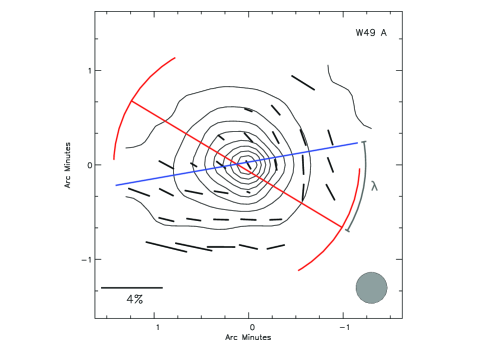
Figure 1: Observations of molecular cloud W49A. Contours represent the levels of the radio flux. Small black line-segments shows the direction of the magnetic field at the point. Figure is taken from Tassis et al. (2009).

2 Magnetohydrodynamics equations for weakly ionized gas

For description of gas motion in molecular clouds one can use two-fluid hydrodynamic equations. We denote velocities of a neutral and an ionized gas components as $\bf v$ and $\bf u$ respectively. Magnetic viscosity $\nu_{m}$ in molecular clouds is much less than the kinematic viscosity $\nu$ (see Dogiel et al. 1987).

We consider gas motions on the scales $L$ corresponding to the inertial range $L_{\nu}<L<L_{0}$, where $L_{0}$ is determined by the size of the system, and $L_{\nu}$ corresponds to the viscous scale. Typical values for molecular clouds are $L_{0}=10^{19}$ cm, Reynolds number is $Re=10^{8}$, hence for the Kolmogorov turbulence $L_{\nu}=L_{0}Re^{-3/4}=10^{13}$ cm. In this range of scales the viscosity can be neglected. Turbulent velocity at small scales is less than the sound velocity, it reaches the value of sound velocity only at large scales. So we assume gas to be incompressible, because subsonic gas motions can be considered to be incompressible. Then equations for the ionized component motion and the magnetic field are

$$\frac{\partial\bf u}{\partial t}+{(\bf u\nabla)u}=\frac{1}{\rho_{i}}\left[-{\bf\nabla}P_{i}+\frac{\bf{(\nabla\times B)\times B}}{4\pi}\right]-$$ (1)

$$-\mu_{in}({\bf u-v}),$$

$$\frac{\partial\bf B}{\partial t}=\bf\nabla\times(u\times B),$$ (2)

$$\nabla\bf u=0,$$

$$\nabla\bf B=0,$$

where $P_{i}$ and $\rho_{i}$ are the pressure and the density of ionized component, $\mu_{in}$ is ion-neutral collision rate. In contrast to the usual magnetohydrodynamics, in this case an external force in the form of friction between the ionized and the neutral gas components is present. Indeed, estimations give

$$\mu_{ni}=10^{-13}\,\text{s}^{-1},\qquad\mu_{in}=2\cdot 10^{-6}\,\text{s}^{-1},$$ (3)

whereas the turbulent fluctuation frequencies lie in the range

$$\omega_{min}=10^{-12}\,\text{s}^{-1},\qquad\omega_{max}=10^{-8}\,\text{s}^{-1}.$$ (4)

This implies an important condition

$$\mu_{ni}\ll\omega\ll\mu_{in}.$$ (5)

This means that the neutral gas does not feel the presence of an ionized component. Ions motion, by contrast, is completely determined by the motion of a neutral gas. Numerical estimates of the characteristic frequencies of the problem were discussed in detail by Dogiel et al. (1987).

Thus we can treat the motion of the neutral component to be known, it coincides with the ordinary hydrodynamic turbulence. For an ionized component only two forces are essential: the force of friction on a neutral gas and the Lorentz force, caused by a magnetic field. As we will see below, the pressure $P_{i}$ can be neglected in comparison with the pressure of the magnetic field. Therefore the motion equation for an ionized component becomes

$$\frac{\bf(\nabla\times B)\times B}{4\pi\rho_{i}}-\mu_{in}\bf(u-v)=0.$$ (6)

Let us denote

$$a=\frac{1}{4\pi\rho_{i}\mu_{in}}.$$ (7)

As far as we consider a gas to be incompressible, $a=$ const. Expressing the velocity of an ionized component in terms of velocity of neutrals and substituting it to the induction equation (2), we obtain

$$\frac{\partial\bf B}{\partial t}={\bf\nabla\times(v\times B)}-a\bf\nabla\times(B\times(\nabla\times B)\times B).$$ (8)

This equation gives the dependence of the magnetic field on the velocity $\bf v$ of a neutral gas.

3 Derivation of evolution equation

3.1 Tensor structure of correlators

To describe the turbulent motion of a neutral gas and obtain closed equations for magnetic field correlators, we use solvable model proposed by Kazantsev (1968) and Kraichnan (1968). We assume neutral gas velocity ${\bf v}(t)$ to be a Gaussian stochastic process with zero mean value, $\langle{\bf v}\rangle=0$. All information about it is contained in the pair correlation function $\langle v_{i}({\bf x},t)v_{j}({\bf x+r},t^{\prime})\rangle$. The angle brackets here and below denote averaging over an ensemble of realizations. We assume a neutral gas to be a homogeneous isotropic medium, so the pair correlation function can depend only on $\bf{r}$. We consider the velocity field to be delta-correlated in time,

$$\langle v_{i}({\bf x},t)v_{j}({\bf x+r},t^{\prime})\rangle=v_{ij}({\bf r})\tau_{c}\delta(t-t^{\prime}),$$ (9)

and mirror-symmetric. It possesses no helicity, and its correlation tensor is symmetric with respect to the interchange of indices $v_{ij}({\bf r})=v_{ji}({\bf r})$. In this case one can construct the tensor structure of the correlation function from only two second-rank tensors

$$v_{ij}=2V(r)\delta_{ij}+S(r)(\delta_{ij}-\frac{r_{i}r_{j}}{r^{2}}).$$ (10)

The factor $2$ in the first term of the right hand side is written for convenience. From the incompressibility condition $\nabla\bf{v}=0$, i.e. $\partial_{i}v_{ij}=\partial_{j}v_{ij}=0$, we obtain

$$S=rV^{\prime},$$ (11)

where prime denotes the derivative with respect to $r$, $V^{\prime}=\partial V/\partial r$. This relation leads us to the general form of the correlation tensor

$$v_{ij}(r)=2V(r)\delta_{ij}+rV^{\prime}(r)\left(\delta_{ij}-\frac{r_{i}r_{j}}{r^{2}}\right).$$ (12)

Thus, the neutral gas turbulence is described by one scalar function $V(r)$. A common method to handle this problem is to pass to the Fourier space

$${\bf v(r},t)=\int{\bf v(k},t)\exp(i{\bf kr})d{\bf k}.$$ (13)

Indeed, the correlation tensor structure becomes simplier

$$\langle v_{i}({\bf k},t)v_{j}({\bf k^{\prime}},t^{\prime})\rangle=\overline{V}(k)\tau_{c}\delta(t-t^{\prime})\left(\delta_{ij}-\frac{k_{i}k_{j}}{k^{2}}\right)\delta({\bf k+k^{\prime}}).$$ (14)

The factor $\delta({\bf k+k^{\prime}})$ arises from homogeneity, and the tensor structure is uniquely determined by isotropy and incompressibility condition $k_{i}v_{i}(k)=0$. Functions $V(r)$ and $\overline{V}(r)$ are related by

$$\overline{V}(r)=3V(r)+rV^{\prime}(r),$$ (15)

and $\overline{V}(k)$ is a Fourier transform of $\overline{V}(r)$,

$$\overline{V}(r)=\int\overline{V}(k)\exp(i({\bf kr}))d\bf k.$$ (16)

Now let us consider correlators of the magnetic field. We assume magnetic field to be a Gaussian stochastic process too. But it has nonzero mean value. Let us denote its mean and fluctuating components by $\bf H$ and $\bf b$ respectively:

$$\bf B=H+b,\qquad\langle B\rangle=H.$$ (17)

We suppose mean magnetic field to be constant in space ${\bf H}=\text{const}({\bf r})$. One can look for the evolution equation for ${\bf H}(t)$, using the technique described below, and get $\partial{\bf H}/\partial t=0$. Hence the value of the mean field ${\bf H}=\text{const}({\bf r},t)$ is an external parameter of the problem.

Strictly speaking, magnetic field $\bf B$, generated by the Gaussian stochastic field $\bf v$, is not pure Gaussian. Its properties are not completely described by the second order correlation function. But significant difference appears in higher than second order moments, and for investigation of second order moment evolution one can assume $\bf B$ to be Gaussian, see, for example, the paper by Brandenburg & Subramanian (2000).

To describe fluctuating component of the magnetic field, we introduce its pair correlator $\langle b_{i}({\bf x},t)b_{j}({\bf x+r},t)\rangle$, which is similar to the velocity correlator, but the average is taken at the same time moments. Our aim is to establish the evolution equation for this correlator. Since

$$\frac{\partial}{\partial t}\langle b_{i}b_{j}\rangle=\langle\frac{\partial b_{i}}{\partial t}b_{j}\rangle+\langle b_{i}\frac{\partial b_{j}}{\partial t}\rangle,$$ (18)

one have to calculate $\partial{\bf b}/\partial t$. We suppose that $\langle b_{i}b_{j}b_{k}\rangle=0$. Averaging Eq. (8), subtracting the resulting equation from Eq. (8), we get

$$\frac{\partial\bf b}{\partial t}={\bf\nabla\times[v\times H]+\nabla\times[v\times b]}-a\bf\nabla\times\Bigl{(}H\times[j\times H]+$$

$$+\bf H\times[j\times b]+b\times[j\times H]+b\times[j\times b]\Bigr{)}-$$

$$-{\bf\nabla\times\langle v\times b\rangle}+a\bf\nabla\times\langle H\times[j\times b]+b\times[j\times H]\rangle,$$ (19)

where we use the notation $\bf j=\nabla\times b$ for short.

Last three terms (last line) in Eq. (3.1) give no contribution to $\partial\langle b_{i}b_{j}\rangle/\partial t$, since $\langle\langle\ldots\rangle b_{i}\rangle=\langle\ldots\rangle\langle b_{i}\rangle=0,$ so they can be ignored. Similarly we omit terms in Eq. (3.1), which are proportional to $b^{2}$, because their contribution to the derivative $\partial\langle b_{i}b_{j}\rangle/\partial t$ is proportional to $\langle b^{3}\rangle=0$.

3.2 The case with zero mean field

To begin with we consider the case when the mean field is absent, $H=0$. Then all correlators are isotropic. Maxwell equation $\nabla{\bf b}=0$ is similar to the incompressibility equation $\nabla{\bf v}=0$, so tensor structure of the magnetic field correlator for the non-helical case is similar to the velocity correlator (12)

$$\langle b_{i}({\bf x},t)b_{j}({\bf x+r},t)\rangle=2Q(r)\delta_{ij}+rQ^{\prime}(r)\left(\delta_{ij}-\frac{r_{i}r_{j}}{r^{2}}\right).$$ (20)

In the Fourier space the correlator is

$$\langle b_{i}({\bf k},t)b_{j}({\bf k^{\prime}},t)\rangle=\overline{Q}({\bf k})\left(\delta_{ij}-\frac{k_{i}k_{j}}{k^{2}}\right)\delta(\bf k+k^{\prime}),$$ (21)

where the relation between $Q(r)$ and $\overline{Q}(k)$ is similar to (15). Due to the isotropy $\overline{Q}({\bf k})=\overline{Q}(k)$. To get $\partial\overline{Q}(k)/\partial t$ we apply Fourier transform to Eq. (3.1), drop terms which do not contribute to the value of $\partial\langle b_{i}b_{j}\rangle/\partial t$, put $H=0$ and obtain

$$\begin{split}\frac{\partial\bf b(k)}{\partial t}&=i\int d{\bf q\,k\times[v(q)\times b(p)]}+\\ &+a\int d{\bf k_{1}}d{\bf k_{2}}\,{\bf k\times\{b(k_{1})\times([k_{2}\times b(k_{2})]\times b(k_{3}))}\}.\end{split}$$ (22)

In the first term of the right hand side $\bf p+q=k$, in the second term $\bf k_{1}+k_{2}+k_{3}=k$. One can see the following structure of correlator’s derivative

$$\frac{\partial}{\partial t}\langle bb\rangle\simeq\langle vb^{2}\rangle+\langle b^{4}\rangle,$$ (23)

where only the magnetic field $b$ and the velocity $v$ are shown, and all tensor indices are dropped. We assume random processes $\bf v$ and $\bf b$ to be Gaussian. So, to split the correlators in the first term of Eq. (23) one should use the Furutsu-Novikov formula (see Furutsu 1963; Novikov 1965; Klyatskin 2005). It states that if some functional $R[{\bf v}]$ depends on the random process ${\bf v}({\bf k},t)$ as a solution of some differential equation, one can split correlator

$$\langle v_{i}({\bf k},t)R[{\bf v}]\rangle=\int d{\bf k^{\prime}}dt^{\prime}\,\langle v_{i}({\bf k},t)v_{j}({\bf k^{\prime}},t^{\prime})\rangle\left<\frac{\delta R[{\bf v}]}{\delta v_{j}({\bf k^{\prime}},t^{\prime})}\right>,$$ (24)

where $\langle\delta R[{\bf v}]/\delta v_{j}({\bf k^{\prime}},t^{\prime})\rangle$ is a functional derivative. To compute it one should use the equation which specifies the dependence of $R$ on ${\bf v}$. In our case it is the evolution equation (22). Since the random process ${\bf v}$ is assumed to be delta-correlated in time, and at $t^{\prime}>t$ causality principle states that $\delta b_{i}({\bf k},t)/\delta v_{j}({\bf k^{\prime}},t^{\prime})=0$, we need to know only the value of

$$\lim_{t^{\prime}\to t-0}\quad\frac{\delta b_{i}({\bf k},t)}{\delta v_{j}({\bf k^{\prime}},t^{\prime})}=ik_{m}(\delta_{ij}b_{m}^{{\bf k-k^{\prime}}}-\delta_{jm}b_{i}^{\bf k-k^{\prime}}).$$ (25)

In the right hand side the argument is written as a superscript for clarity. In the second term of Eq. (23) one can presents forth order correlator as a product of pair correlators

$$\langle b_{1}b_{2}b_{3}b_{4}\rangle=\langle b_{1}b_{2}\rangle\langle b_{3}b_{4}\rangle+\langle b_{1}b_{3}\rangle\langle b_{2}b_{4}\rangle+\langle b_{1}b_{4}\rangle\langle b_{2}b_{3}\rangle.$$ (26)

Let us write out the intermediate result obtained after splitting of correlators. To do this, we use the notations

$$\Omega_{ij}^{\bf k}=\delta_{ij}-\frac{k_{i}k_{j}}{k^{2}},$$ (27)

and ${\bf p}=\bf k-q$. We obtain

$$\frac{\partial\overline{Q}(k)}{\partial t}\Omega_{ij}^{\bf k}=2a\int d{\bf q}\,\overline{Q}(k)\overline{Q}(q)\Bigl{(}-k^{2}\Omega^{\bf q}_{is}\Omega^{\bf k}_{sj}-$$ (28)

$$-k_{m}k_{s}\Omega^{\bf q}_{ms}\Omega^{\bf k}_{ij}+k_{m}k_{i}\Omega^{\bf q}_{ms}\Omega^{\bf k}_{sj}\Bigr{)}-\tau_{c}k_{m}\int d{\bf q}\,\overline{V}(q)\overline{Q}(k)\times$$

$$\times\Bigl{(}\Omega^{\bf q}_{is}p_{n}(\delta_{ms}\Omega_{nj}^{\bf k}-\delta_{ns}\Omega_{mj}^{\bf k})-(i\leftrightarrow m)\Bigr{)}+\tau_{c}k_{m}\times$$

$$\times\int d{\bf q}\,\overline{V}(q)\overline{Q}(p)\,\Bigl{(}\Omega^{\bf q}_{is}k_{n}(\delta_{js}\Omega_{nm}^{\bf p}-\delta_{ns}\Omega_{mj}^{\bf p})-(i\leftrightarrow m)\Bigr{)}.$$

Tensors in right hand side of last equation contain vectors $q_{i}$ and $p_{i}$, which are absent in the left hand side. To extract the factor $\Omega_{ij}^{\bf k}$ in the right hand side one can use isotropy of $\overline{V}(q)$ and $\overline{Q}(k)$, then average first two integrals over the sphere $|\bf q|=\text{const}$ and the third integral over a circle, determined by conditions $|\bf q|=\text{const}$ and $|\bf p|=\text{const}$. After that tensor factors are cancelled and we get scalar evolution equation

$$\begin{split}\frac{1}{\tau_{c}}\frac{\partial\overline{Q}(k)}{\partial t}=&-\frac{2}{3}k^{2}\overline{Q}(k)\int\,\overline{V}(q)d{\bf q}+\\ &+k^{2}\int\,\overline{V}(q)\overline{Q}(p)\left[1-\frac{({\bf kp})({\bf kq})({\bf pq})}{k^{2}p^{2}q^{2}}\right]d{\bf q}-\\ &-\frac{2}{3\pi\rho_{i}\mu_{in}\tau_{c}}k^{2}\overline{Q}(k)\int\,\overline{Q}(q)d{\bf q},\end{split}$$ (29)

where ${\bf k}=\bf p+q$. This equation was derived firstly by Dogiel et al. (2005). Let’s introduce the notation

$$\lambda=\frac{1}{3\pi\rho_{i}\mu_{in}\tau_{c}}\int\,\overline{Q}(q)d{\bf q}.$$ (30)

The value of $\lambda$ is proportional to $b_{0}^{2}=\langle b_{i}({\bf x})b_{i}({\bf x})\rangle$ which is the energy of the fluctuating magnetic field.

Since solving the integral equation on $\overline{Q}(k)$ in the $k$-space is rather complicated problem, let us turn back to the $r$-space and obtain the differential equation for $Q(r)$. To do this, we apply inverse Fourier transform to the Eq. (29). One can express the value of parameter $\lambda$ in terms of $Q(r)$

$$\lambda=\frac{4}{3}\frac{a}{\tau_{c}}\overline{Q}(r=0)=\frac{2a}{\tau_{c}}(2Q(r)+\frac{2}{3}rQ^{\prime}(r))|_{r\to 0}.$$ (31)

Also note that

$$V(0)=\frac{1}{3}\int\,\overline{V}(q)d\bf q.$$ (32)

We proceed from functions $\overline{Q}(r)$, $\overline{V}(r)$ to $Q(r)$, $V(r)$ according to Eq. (15), use the spherical symmetry of the correlation functions and get after some algebra

$$\begin{split}\frac{1}{2\tau_{c}}\frac{\partial Q(r)}{\partial t}=&\left(V(0)-V(r)+\lambda\right)(Q^{\prime\prime}+\frac{4Q^{\prime}}{r})-\\ &-V^{\prime}Q^{\prime}-\frac{1}{r}(4V^{\prime}+rV^{\prime\prime})Q.\end{split}$$ (33)

One of the key points of this derivation is averaging over a sphere (or circle), when we use the isotropy of the functions $\overline{V}(q)$ and $\overline{Q}(k)$. In the anisotropic case, in the presence of the mean field, for example, this averaging fails. Thus, we conclude that in general case it is necessary to derive and solve the evolution equation in $r$-space. It is no need to apply a Fourier transform. Tensor structure of correlators (12) in this method is more complicated, but there arise no integral equations and additional vectors (as $p_{i}$, $q_{i}$) in the tensor structure.

Indeed, the equation (33) can be obtained directly in the $r$-space, by analogy with the above derivation. We will discuss its solution in the section 4.2.

3.3 The general case of a non-zero mean field $H\neq 0$

In this part we consider general case when the mean magnetic field is present. The correlation function of magnetic fluctuations becomes anisotropic. We assume magnetic field to have no helicity, so its correlation tensor $\langle b_{i}b_{j}\rangle$ is symmetric with respect to the interchange of indices. We suppose that it has the form

$$\begin{split}\langle b_{i}({\bf x},t)b_{j}({\bf x+r},t)\rangle&=A({\bf r})\delta_{ij}+B({\bf r})n_{i}n_{j}+\\ &+C({\bf r})(n_{i}h_{j}+n_{j}h_{i})+D({\bf r})h_{i}h_{j},\end{split}$$ (34)

where ${\bf n}={\bf r}/r$, ${\bf h}={\bf H}/H$ are unit vectors in the directions of $\bf r$ and $\bf H$ respectively.

The most general form of the correlation tensor of the second order in the presence of a preferred direction of the mean magnetic field is given in the paper by Matthaeus & Smith (1981). However, we restrict our attention to terms, specified in Eq. (34). As we will see below this assumption is consistent, in the right hand side of evolution equations only the same tensor terms arise.

All scalar functions are no longer spherically symmetric, but they are axially symmetric with respect to the direction of $\bf H$. We choose this direction as $z$-axis. Below spherical coordinates $(r,\,\mu=\cos\theta)$ are used, where $\theta$ is the polar angle between $\bf n$ and $\bf h$.

From the symmetry of the correlator and homogeneity of space, functions $A,B,D$ should be symmetric with respect to $\mu$, $A(r,\,\mu)=A(r,\,-\mu)$, whereas function $C$ should be anti-symmetric $C(r,\,\mu)=-C(r,\,-\mu)$.

Condition $\nabla{\bf b}=0$ gives us two relations

$$A^{\prime}_{r}-\frac{\mu}{r}A^{\prime}_{\mu}+B^{\prime}_{r}+\mu C^{\prime}_{r}+\frac{1-\mu^{2}}{r}C^{\prime}_{\mu}+\frac{2B}{r}-\frac{\mu C}{r}=0$$

$$\frac{1}{r}A^{\prime}_{\mu}+C^{\prime}_{r}+\mu D^{\prime}_{r}+\frac{1-\mu^{2}}{r}D^{\prime}_{\mu}+\frac{3C}{r}=0.$$ (35)

The derivation of the evolution equations is similar to that performed in the previous section, but now we work in the $r$-space. We use Eq. (3.1) instead of Eq. (22) and the functional derivative

$$\frac{\delta b_{i}({\bf r},t)}{\delta v_{j}({\bf r^{\prime}},t-0)}=\frac{\partial}{\partial r_{m}}\left(\delta({\bf r-r^{\prime}})(B_{m}({\bf r})\delta_{ij}-B_{i}({\bf r})\delta_{jm})\right),$$ (36)

where $\bf B=H+b$ is total magnetic field, instead of the formula (25). As before, we use the relation

$$\langle b_{i}({\bf r})\frac{d}{dr}b_{j}({\bf r})\rangle=0.$$ (37)

which is due to the symmetry of the correlator and homogeneity of space. Finally one principally can write out the bulky system of evolution equations (for the functions $A,B,C,D$), which contains the second order derivatives in the right hand side. It must be solved taking into account relations (3.3). To solve such a system would be very difficult. To simplify this system, one can use the structure of the Eq. (8), and split the system of equations with second-order spatial derivatives into two systems with first-order derivatives. Namely, we replace one of the unknown functions by

$$\tilde{D}=D+H^{2},$$ (38)

introduce the notations

$$X = a(D(0)+H^{2})=a\tilde{D}(0)$$ (39)

$$Y(r) = -2aA(0)+\tau_{c}(V(r)-V(0)+\frac{1}{2}rV^{\prime})$$

and get

$$\begin{split}&\frac{\partial}{\partial t}\langle b_{k}({\bf x})b_{j}({\bf x+r)}\rangle=e_{ksi}\partial_{s}\Bigl{(}f_{1}h_{m}e_{ijm}+f_{2}[{\bf nh}]_{i}h_{j}+\\ &f_{3}[{\bf nh}]_{i}n_{j}+f_{4}n_{m}e_{ijm}\Bigr{)}+\Bigl{(}j\leftrightarrow k,{\bf r\leftrightarrow(-r)}\Bigr{)}=0,\end{split}$$ (40)

where $e_{ksi}$ is the completely anti-symmetric pseudo-tensor, and

$$f_{1} = X(\mu A^{\prime}_{r}+\frac{1-\mu^{2}}{r}A^{\prime}_{\mu}-\frac{\mu B+C}{r})+Y(-\frac{1}{r}A^{\prime}_{\mu}+\frac{C}{r})-$$ (41)

$$-(3V^{\prime}+rV^{\prime\prime})(C+\mu\tilde{D})$$

$$f_{2} = -X(A^{\prime}_{r}-\frac{\mu}{r}A^{\prime}_{\mu}-\frac{B}{r})+(X-Y)\frac{1}{r}C^{\prime}_{\mu}-$$

$$-(X-Y+rV^{\prime})\tilde{D}^{\prime}_{r}+(X-Y)\frac{\mu}{r}\tilde{D}^{\prime}_{\mu}+V^{\prime}\tilde{D}$$

$$f_{3} = (X-Y)\frac{1}{r}B^{\prime}_{\mu}-(X-Y+rV^{\prime})C^{\prime}_{r}+(X-Y)\frac{\mu}{r}C^{\prime}_{\mu}+$$

$$+\frac{1}{r}(X-Y+r^{2}V^{\prime\prime})C-(V^{\prime}-rV^{\prime\prime})\mu\tilde{D}$$

$$f_{4} = (rV^{\prime}-Y)A^{\prime}_{r}+Y(\frac{\mu}{r}A^{\prime}_{\mu}+\frac{B}{r})-V^{\prime}A-$$

$$-(3V^{\prime}+rV^{\prime\prime})(A+B+\mu C).$$

Let us note that the correlator of the form (34) with function $\tilde{D}$ instead of $D$ in the right hand side describes the correlator of the total magnetic field $\langle B_{i}B_{j}\rangle$. The system of evolution equations with nonzero mean field is not homogeneous, it contains a "source" term, which is proportional to $H^{2}$. However, the system with function $\tilde{D}$ is homogeneous, but the term with $H^{2}$ arises in boundary conditions.

From Eq. (40) one can obtain evolution equations:

$$\frac{1}{2}\frac{\partial A}{\partial t} = \mu\partial_{r}f_{1}+\frac{1-\mu^{2}}{r}\partial_{\mu}f_{1}+\partial_{r}f_{4}+\frac{f_{4}}{r}$$ (42)

$$\frac{1}{2}\frac{\partial B}{\partial t} = \mu\partial_{r}f_{3}+\frac{1-\mu^{2}}{r}\partial_{t}f_{3}-2\mu\frac{f_{3}}{r}-\partial_{r}f_{4}+\frac{\mu}{r}\partial_{\mu}f_{4}+\frac{f_{4}}{r}$$

$$\frac{1}{2}\frac{\partial C}{\partial t} = \frac{1}{2}\Bigl{(}-\partial_{r}f_{1}+\frac{\mu}{r}\partial_{\mu}f_{1}+\mu\partial_{r}f_{2}+\frac{1-\mu^{2}}{r}\partial_{\mu}f_{2}-\mu\frac{f_{2}}{r}-$$

$$-\partial_{r}f_{3}-\frac{1}{r}\partial_{\mu}f_{4}\Bigr{)}$$

$$\frac{1}{2}\frac{\partial D}{\partial t} = -\Bigl{(}\frac{1}{r}\partial_{\mu}f_{1}+\partial_{r}f_{2}+\frac{f_{2}}{r}\Bigr{)}.$$

We restrict ourselves to search for stationary solutions. In this case, the time derivatives are equal to zero, and the system (42) can be solved exactly. Its solution depends on one arbitrary function $g(r,\mu)$

$$f_{1} = -g^{\prime}_{r}$$ (43)

$$f_{2} = \frac{1}{r}g^{\prime}_{\mu}$$

$$f_{3} = g^{\prime}_{r}-\frac{\mu}{r}g^{\prime}_{\mu}-\frac{g}{r}$$

$$f_{4} = \mu g^{\prime}_{r}+\frac{1-\mu^{2}}{r}g^{\prime}_{\mu}-\frac{\mu g}{r}.$$

From Eq. (41) and (43), taking into account two relations (3.3), we get six first-order equations for five unknown functions $A,B,C,\tilde{D},g$. The single boundary condition is $A,B,C,D\to 0$ when $r\to\infty$ because the pair correlation function of magnetic field fluctuations should vanish at large scales.

The system of six equations for five unknown functions seems overdetermined and has no solutions at first glance. However, if $H\gg 1$ this system can be simplified considerably and allows the analytical solution, which is given in section 4.4. In this limit case the system is degenerate and is not overdetermined. This suggests that the same would takes place in the general case.

3.4 Small mean field $H$

Because of the large complexity of equations in the anisotropic case, we consider firstly a simpler problem, we assume that the correlator $\langle b_{i}b_{j}\rangle$ is isotropic, i.e. it has the form (20) even in the case $H\neq 0$. This can be done in the case of small mean field $H$, because, as we will see below, if $H^{2}\ll\tau_{c}\rho_{i}\mu_{in}v_{0}^{2}$, the amplitude of the fluctuations $b_{0}\sim H^{1/2}$ is greater than $H$.

To get isotropic equations we have to replace

$$h_{i}h_{j}\Longrightarrow\frac{1}{3}\delta_{ij}.$$

Evolution equation becomes

$$\begin{split}\frac{1}{2\tau_{c}}\frac{\partial Q(r)}{\partial t}=&\left(V(0)-V(r)+\lambda+\frac{2a}{\tau_{c}}\frac{H^{2}}{3}\right)(Q^{\prime\prime}+\frac{4Q^{\prime}}{r})-\\ &-V^{\prime}Q^{\prime}-\frac{1}{r}(4V^{\prime}+rV^{\prime\prime})(Q+\frac{1}{6}H^{2}),\end{split}$$ (44)

where as before

$$\lambda=\frac{2a}{\tau_{c}}(2Q(0)+\frac{2}{3}rQ^{\prime}(r)|_{r\to 0}).$$ (45)

When $H=0$ Eq. (44) turns into Eq. (33).

4 The solution of equations

4.1 Preliminaries

Let us reduce our equation to dimensionless one. Before that we denote the rms velocity of the neutral gas by $v_{0}$, $v_{0}^{2}\leavevmode\nobreak\ =\leavevmode\nobreak\ \langle v_{i}({\bf x})v_{i}({\bf x})\rangle=6V(0)$, and the rms amplitude of the magnetic field fluctuations by $b_{0}$, $b_{0}^{2}=\langle b_{i}({\bf x})b_{i}({\bf x})\rangle$. The correlation time of the velocity field assumed to be equal to $\tau_{c}=\tau_{max}=L_{0}/v_{0}$. That is the eddy turnover time at scale $L_{0}$. For length unit we take the size of the molecular cloud $L_{0}$, for unit of time we take $\tau_{max}$, and for unit of magnetic field we take the value of

$$B_{unit}=\left(\frac{\tau_{c}}{2a}V(0)\right)^{1/2}=\left(\frac{\pi}{3}L_{0}v_{0}\rho_{i}\mu_{in}\right)^{1/2}.$$

In other words, we introduce new functions and variables

$$\begin{split}&r^{(1)}=r/L_{0};\quad t^{(1)}=t/\tau_{max};\\ &V^{(1)}(r)=V(r)/V(0);\quad Q^{(1)}(r)=Q(r)/\left(\frac{\tau_{c}}{2a}V(0)\right).\end{split}$$ (46)

Thus, we reduce Eq. (44) to the form (below we omit superscript (1))

$$\begin{split}3\,\frac{\partial Q(r)}{\partial t}=&\left(V(0)-V(r)+\lambda+\frac{1}{3}H^{2}\right)(Q^{\prime\prime}+\frac{4Q^{\prime}}{r})-\\ &-V^{\prime}Q^{\prime}-\frac{1}{r}(4V^{\prime}+rV^{\prime\prime})(Q+\frac{1}{6}H^{2}).\end{split}$$ (47)

where $\lambda=2Q(0)+\frac{2}{3}rQ^{\prime}(r)|_{r\to 0}$, and $V(0)=1$. For typical parameters of molecular clouds

$$\begin{split}&N_{n}\simeq 10^{3}\,\text{cm}^{-3};\quad N_{i}\simeq 10^{-2}\,\text{cm}^{-3};\quad\\ &L_{0}\simeq 3\cdot 10^{18}\,\text{cm};\quad\,v_{0}\simeq 1\,\text{km/s};\quad T\simeq 50K,\end{split}$$ (48)

the unit of magnetic field is equal to $B_{unit}\leavevmode\nobreak\ \simeq\leavevmode\nobreak\ 200\,\mu G$. But the cloud parameters change in a wide range, so values of $B_{unit}$ for them can vary significantly.

Let us estimate the characteristic scales of our problem. The inertial range of the turbulence is (in the dimensionless variables)

$$l_{\nu}<r<1,$$ (49)

where $l_{\nu}=Re^{-3/4}=10^{-6}$ is the viscous scale. Since in the stationary case the magnetic field energy on one hand is less than the kinetic energy of a neutral gas, but on the other hand is larger than the kinetic energy of an ionized gas, then

$$10^{-6}\simeq\frac{\omega_{min}}{\mu_{in}}=(\tau_{c}\mu_{in})^{-1}\ll\lambda<(\tau_{c}\mu_{ni})^{-1}=\frac{\omega_{min}}{\mu_{ni}}\simeq 10.$$

Therefore, we can consider $l_{\nu}\ll\lambda^{1/\alpha}$.

Let us examine the dimensionless equation (47). The parameter $\lambda$ contains the value of $Q(0)$, so this equation is nonlinear. Let us suppose that the initially magnetic field fluctuations are weak (and the parameter $\lambda$ is small). Then the term, which is proportional to $H^{2}$, makes the positive contribution to the value of $\partial Q/\partial t$, and lead to the initial growth of the magnetic field. Further, this growth will be stopped by nonlinear terms. So we restrict ourselves looking for stationary solutions only. Investigation of a stability of these solutions, especially for anisotropic equations (41), (42), is beyond the scope of our paper.

Since for the stationary solution the parameter $\lambda$ does not depend on time, we will initially consider it to be a constant, which is not connected with the function $Q(r)$. The single restriction is $\lambda>0$, because of $3\lambda=b_{0}^{2}$ (in dimensionless variables). Under such approach the equation (47) becomes linear.

The similar linear equation arises in the problem of magnetic dynamo in a turbulent conducting media. In this problem the parameter $\lambda$ corresponds to the magnetic viscosity and is considered to be known. The equation, coinciding with Eq. (47), was investigated in large number of papers beginning from the paper by Kazantsev (1968), where the integral equation, similar to Eq. (29), was derived. The brief literature review and necessary references are given in the Discussion. In most of the papers the mean magnetic field was considered to be zero. In order to reveal the role of the mean magnetic field we discuss separately cases $H=0$ and $H\neq 0$.

To resolve our equations we need to determine the function $V(r)$ which characterizes the motion of a neutral gas. The value of $L_{0}$ corresponds to the maximum scale of the turbulence. It means that the correlation of gas velocities vanishes at the such scale. We consider the velocity spectrum of a neutral gas to be the power law. So, the correlation function of gas velocities is

$$V(r)=\begin{cases}1-r^{\alpha},&r<1\\ 0,&r>1.\end{cases}$$ (50)

Hereinafter we consider the Kolmogorov turbulence. In this case velocity fluctuation on the scale $r$ is $v(r)\sim r^{1/3}$ in the inertial range, hence $\alpha=2/3$. On the viscous scales $r<l_{\nu}$ velocity fluctuations are $v(r)\sim r$. Therefore the correlation function is $V(r)=\leavevmode\nobreak\ 1-Cr^{2}$. Because $l_{\nu}=10^{-6}$ and we consider $(l_{\nu})^{\alpha}\ll\lambda$, then in this range the correlation function is approximately constant, $V(r)\approx 1$, and the sought correlation function of the magnetic field is, $Q(r)\approx Q(0)$, too. The exclusion is solution $Q(r)$ which have singularity at $r=0$. But we do not consider such solutions (see below). Thus, the viscous range of scales does not affect the further analysis.

Figure 2: The preferential solution $Q(r)$ for different values of the mean magnetic field $H$

Let us note that in the Kazantsev-Kraichnan model the turbulent velocity is assumed to be $\delta$-correlated in time (9) with some value of the correlation time $\tau_{c}$. Because $\tau_{c}$ characterizes the total realization of the turbulent motion, it formally can not be a function of the scale $r$. However, many authors who apply the Kazantsev-Kraichnan model to the problem of magnetic dynamo, in order to approach the physical reality, consider $\tau_{c}$ to be a function of the scale. They assume $\tau_{c}$ to be equial to the turnover time at given scale, $\tau_{c}(r)\sim r/\langle v^{2}\rangle^{1/2}_{r}$. In this case $V(r)\sim r\langle v^{2}\rangle^{1/2}_{r}$ and the Kolmogorov turbulence corresponds to the value $\alpha=4/3$. This assumption is justified by the comparison of theoretical results in the model $\alpha=4/3$ with numerical simulations of forced Navier–Stokes equation (Mason et al. 2011; Tobias,Cattaneo & Boldyrev 2013).

From the theoretical point of view, Vainshtein & Kichatinov (1986) and Boldyrev & Cattaneo (2004) state that we need to know only the integral of the velocity correlation function over time, that is, the turbulent diffusivity, which in Kolmogorov turbulence scales as $r^{4/3}$.

In current paper we use the Kazantsev-Kraichnan model (9) considering $\tau_{c}=\text{const}(r)$.

Figure 3: The dependence of $b_{0}$ on $H$. The dashed line $b_{0}=H$ is given for orientation

4.2 The case with zero mean field

To begin with we consider the case of zero mean magnetic field. We put $\partial Q/\partial t=0$ and $H=0$ in Eq. (47) and we obtain second order equation for the function $Q(r)$

$$\left(V(0)-V(r)+\lambda\right)(Q^{\prime\prime}+\frac{4Q^{\prime}}{r})-V^{\prime}Q^{\prime}-\frac{1}{r}(4V^{\prime}+rV^{\prime\prime})Q=0,$$ (51)

where $\lambda=2Q(0)+\frac{2}{3}rQ^{\prime}(r)|_{r\to 0}$. In this expression the term $rQ^{\prime}(r)$ is essential only for solutions which have singularity at $r=0$. The boundary condition is $Q\to 0$ at $r\to\infty$.

Eq. (51) has two independent solutions. At $r\to 0$ ($l_{\nu}\ll r\ll\lambda^{1/\alpha}$) one can find the asymptotics of the solutions, and at $r>1$ Eq. (51) can be solved exactly

$$r\to 0 : \qquad Q_{1}\sim 1;\qquad Q_{2}\sim r^{-3}$$ (52)

$$r>1 : \qquad Q_{1}=1;\qquad Q_{2}=r^{-3}.$$

Now let us discuss the existence of the solution which is bounded at $r=0$ and is decreasing at $r\to\infty$. At the same time we can consider more general nonstationary equation, where we assume $\lambda$ to be independent of time constant as before. Making the substitution

$$Q(r,t)=\frac{\Psi(r)}{r^{2}}(m(r))^{1/2}\,e^{-Et},$$ (53)

where $m(r)^{-1}=V(0)-V(r)+\lambda>0$, we get for the function $\Psi(r)$ the Shrödinger equation with the variable mass $m(r)$

$$\frac{1}{m(r)}\frac{d^{2}\Psi}{dr^{2}}+(E-U(r))\Psi=0.$$ (54)

The such substitution was firstly done by Kazantsev (1968). The reduction to the Shrödinger equation was discussed in detail in the paper by Schekochihin, Boldyrev & Kulsrud (2002). The stationary solution corresponds to $E=0$, the negative values of the energy $E$ mean the exponential growth of the magnetic field. For the chosen velocity correlator $V(r)$ (50) one can obtain the analytic expression for the potential $U(r)$. For $\alpha<0.915$ (that includes the Kolmogorov turbulence) the potential $U(r)$ is positive everywhere. Hence there is no solutions exponentially growing with time. Eq. (51) also has no finite at $r=0$ and vanishing at $r\to\infty$ solution. Consequently any solution $Q(r)$ has the same power asymptotics (52) at $r\to 0$ and at $r\to\infty$. The solution $Q_{1}$ of the stationary equation, which is finite at $r=0$, falls down at $r\to\infty$ not to zero, but to some positive value. We demand $Q\to 0$ at $r\to\infty$. Only the solution $Q_{2}$, which has singularity at $r=0$, satisfies this condition. This solution has the power law behavior $r^{-3}$ even at scales $r<l_{\nu}$, up to very small scales where the magnetic viscosity becomes important. Thus, there is no finite solutions with the zero mean magnetic field for the Kolmogorov turbulence ($\alpha=2/3$).

For $\alpha>0.915$ and $\lambda<\lambda_{max}(\alpha)$ there exists the region where $U(r)<0$. There appears the bound states, i.e. finite solutions of the Shrödinger equation with $E<0$. That means that the magnetic field will grow up to the level when $\lambda=\lambda_{max}$.

Figure 4: The dependence of the correlation length $l_{corr}$ on $H$

4.3 Small mean field $H$

Now we look for stationary solutions of Eq. (47) with small but nonzero mean magnetic field. This equation is inhomogeneous one, and its partial solution is a constant, $Q(r)=-H^{2}/6$. We introduce the quantity

$$\tilde{Q}=Q+\frac{1}{6}H^{2},$$ (55)

denote $\lambda^{\prime}=\lambda+\frac{1}{3}H^{2}$, and obtain for the $\tilde{Q}$ exactly the homogeneous equation (51) with the replacement $\lambda\rightarrow\lambda^{\prime}$. In fact, the quantity $\tilde{Q}$ is the correlation function of the total magnetic field $\bf B=H+b$

$$\langle B_{i}({\bf x})B_{j}({\bf x+r})\rangle=\langle b_{i}({\bf x})b_{j}({\bf x+r})\rangle+\frac{1}{3}H^{2}\delta_{ij}.$$ (56)

The last term is written in the form $\langle H_{i}H_{j}\rangle=H^{2}\delta_{ij}/3$, because in this subsection we assume correlators to be isotropic. Therefore, the tensor structure of the correlator $\langle B_{i}B_{j}\rangle$ coincides with (20). It is possible to derive evolution equation directly for this correlator, including the mean magnetic field, as was done by Boldyrev, Cattaneo & Rosner (2005). However, the boundary conditions for $\tilde{Q}$ are different

$$2\tilde{Q}(0)+\frac{2}{3}r\tilde{Q}^{\prime}|_{r\to 0}=\lambda^{\prime}$$ (57)

$$\tilde{Q}\to\frac{1}{6}H^{2},\qquad r\to\infty,$$ (58)

because of the fluctuations correlator tends to zero at large distances, but the correlator $\langle H_{i}H_{j}\rangle$ is independent on the distance due to its homogeneity.

Figure 5: Functions $A_{0}(r)$-thick line, $B_{0}(r)$-thin, $D_{0}(r)$-dashed, $D_{1}(r)$- dotted lines

As was mentioned in the previous subsection, the solution of the stationary equation (51), which is finite at $r=0$, tends to a positive constant at $r\to\infty$. It is in accordance with the new boundary condition (58). Now even for $\alpha=2/3$ there exists the unique bounded solution, we will call it as the preferential solution. The value of $\lambda$ for them is defined by unique manner. Graphs of this solution for three values of the mean magnetic field $H=1$, $H=0.1$ and $H=0.01$ are presented on the Fig. 2. These graphs and all other numerical results are obtained for the Kolmogorov turbulence, $\alpha=2/3$. Since

$$\langle b_{i}({\bf x})b_{i}({\bf x})\rangle=b_{0}^{2}=3\lambda,$$ (59)

we get the dependence of $b_{0}$ on $H$, which is presented on the Fig. 3. For $H<1$ the amplitude of the fluctuating magnetic field $b_{0}\sim\sqrt{H}$. Thus, for $H\ll 1$ we have $b_{0}\gg H$, i.e. the fluctuating field dominates over the mean field.

Let us note that for $H\to 0$ the amplitude of the magnetic fluctuations $b_{0}$ for the preferential solution tends to zero also. For $H=0$ the preferential solution turns to the zero solution of equation without the mean field. It corresponds to the fact that for $H=0$ there are no bounded solutions vanishing at large scales.

For small values of $r$, $r\ll 1$, the asymptotic behavior of the preferential solution is $Q(r)\simeq Q(0)(1-r^{\alpha}/\lambda)$. In the k-space it gives $k^{2}\overline{Q}(k)\sim k^{-5/3}$ for $\alpha=2/3$, i.e. the magnetic fluctuations spectrum coincides with the spectrum of the hydrodynamic turbulence of a neutral gas.

For the preferential solution one can also calculate the correlation length of the fluctuating magnetic field, which we define by the formula

$$l_{corr}=\frac{1}{b_{0}^{2}}\int_{0}^{\infty}\langle b_{i}({\bf 0})b_{i}({\bf r})\rangle dr.$$ (60)

The numerical results are shown on the Fig. 4. One may note that $l_{corr}\sim H$ for small values of $H$.

Figure 6: Functions $C_{0}(r)$-thick line, $A_{1}(r)$-thin, $B_{1}(r)$-dashed lines

4.4 Large mean field $H$

For large mean field, $H\gg 1$ (in dimensionless units), the correlators of the fluctuating magnetic field can not be considered as isotropic. We need to solve the system of anisotropic equations (3.3),(41) and (43). To reduce this system to dimensionless variables (46) one must change only the relations (39) for values $X,Y$:

$$X = D(0)+H^{2}=\tilde{D}(0)$$

$$Y(r) = -2A(0)+2V(r)-2V(0)+rV^{\prime}.$$

We assume the correlators $A,B,C,D$ to be the order of unity, and keep only terms of $H^{2}\gg 1$ order. The system of equations is simplified significantly. The solution is described in detail in the Appendix A. It turns out that this system of equations is not overdetermined. The dependence of the correlation functions over the angle $\theta$ is simple

$$A(r,\mu) = A_{0}(r)+A_{1}(r)\mu^{2}$$ (61)

$$B(r,\mu) = B_{0}(r)+B_{1}(r)\mu^{2}$$

$$C(r,\mu) = C_{0}(r)\mu$$

$$D(r,\mu) = D_{0}(r)+D_{1}(r)\mu^{2}.$$

where $\mu=\cos\theta$. If we take the correlator $V(r)$ in the form (50), as before, then we obtain a solution which is presented on Fig. 5, 6. We see that the function $D_{1}(r)$ is discontinuous at $r=1$. It is due to the break of the function $V(r)$ at $r=1$, (50). If we choose the correlator $V(r)$, which has the continuous derivative at $r=1$, then values of $A,B,C,D$ will be also continuous, and the function $D_{1}(r)=0$ (see the Appendix A). The obtained solution in this case is shown on the Fig. 7, 8. For small values of $r\ll 1$ the solution include terms $r^{\alpha}$ and $r^{2}$. In the $k$-space they correspond to terms $k^{-11/3}$ and $k^{-5}$ in $\overline{Q}(k)$.

5 Discussion

The problem of the kinematic dynamo in a conducting medium (hereinafter - DCM) is discussed widely. See, for example, papers: Schekochihin et al. (2002); Boldyrev & Cattaneo (2004); Rogachevskii & Kleeorin (1997); Kleeorin & Rogachevskii (2012), Schleicher et al. (2013) and references therein. Also the problem of magnetic field generation in weakly ionized incompressible gas was studied by Subramanian (1997). For analytical treatment the model of Kazantsev-Kraichnan (Kazantsev 1968; Kraichnan 1968) is usually used. At the initial stage of the magnetic field growth its influence on the medium motion is negligible. Therefore, our problem and the problem of DCM are similar in many aspects. In the problem of DCM the evolution equation for the magnetic field is

$$\frac{\partial\bf B}{\partial t}={\bf\nabla\times(v\times B)}+\nu_{m}\Delta\bf B,$$ (62)

where $\nu_{m}$ is the magnetic viscosity. Our Eq. (8) contains the additional term, which is proportional to $B^{3}$, due to the friction between neutral and ionized gases. The term $\nu_{m}\Delta\bf B$ in our case is much smaller than the term $B^{3}$ because of high conductivity, and we omit it. Thus, Eq. (62) and Eq. (8) differ by the last terms only. So, evolution equations for the magnetic field correlators used in papers cited above almost identical with our Eq. (33). Instead of unknown parameter $\lambda$ (45) (it is the averaged square of the amplitude of magnetic field fluctuations) equations of DCM contain the magnetic viscosity $\nu_{m}$ which is considered to be known. Equations of DCM theory are linear, and the problem is to find solutions exponentially growing in time. The dependence of the largest growth rate on $\nu_{m}$ is discussed in Kleeorin & Rogachevskii (2012), Schleicher et al. (2013). Our equation (8) and evolution equation for correlators (33) are nonlinear because the value of $\lambda$ is defined by the solution. This nonlinearity stops the initial growth of magnetic fluctuations. Therefore we are looking for stationary solutions only.

Figure 7: Functions $A_{0}(r)$-thick line, $B_{0}(r)$-thin, $D_{0}(r)$-dashed lines for the smooth correlator $V(r)$

The main result of our paper is taking into account the mean magnetic field, and derivation of evolution equations for anisotropic correlators $\langle bb\rangle$. In all mentioned papers magnetic field correlators were suggested to be isotropic, as in section 3.4 of current work. Rogachevskii & Kleeorin (1997) tried to take into account a mean magnetic field. But when they derive the evolution equation for pair correlators, they put mean field to zero. Boldyrev et al. (2005) made no assumption of zero mean magnetic field. They considered the pair correlator of the total magnetic field $\tilde{Q}\simeq\langle BB\rangle$. Obtained evolution equation for $\tilde{Q}$ coincides with Eq. (33) of our paper for $Q$ (see section 4.3). However, the boundary conditions for $\tilde{Q}$ are different. We consider the media is uniform and the mean magnetic field is constant, so the correlator $\langle H({\bf 0})H({\bf r})\rangle$ is independent of ${\bf r}$. At the same time, the correlator of magnetic field fluctuations must vanish at large scales. So, $Q(r)\to 0$, but $\tilde{Q}(r)\to H^{2}/6$ at $r\to\infty$. As we show in the section 4.3, this difference is essential for existence of bounded solutions.

In all mentioned papers the velocity correlation function was assumed to be $V(r)=1-r^{\alpha}$. In the model with scale-independent correlation time $\tau_{c}$ for the Kolmogorov turbulence $\alpha=2/3$, and, as we show, there are no solutions exponentially growing in time, see also Rogachevskii & Kleeorin (1997). If $\tau_{c}$ is supposed to be a function of the scale, the Kolmogorov turbulence corresponds to $\alpha=4/3$ and growing solutions of (33) appear. This is equivalent to the appearance of solutions of stationary equation (51) bounded at $r=0$ and vanishing at large scales. In current work we demonstrate that when mean field is taken into account, bounded solutions do exist even in the model with $\alpha=2/3$.

Figure 8: Functions $C_{0}(r)$-thick line, $A_{1}(r)$-thin, $B_{1}(r)$-dashed lines for the smooth correlator $V(r)$

6 Conclusion

We find the correlation function of fluctuating magnetic field when the mean magnetic field equals zero, $H=0$. For the Kolmogorov turbulence the correlation function diverges as $r^{-3}$ when $r\to 0$ up to small resistive scales.

For the case $H\neq 0$ the problem is solved in the approximation of isotropic correlators. It is shown that for each value of $H$ there exists the unique solution bounded at $r=0$. When $H<1$ the amplitude of the fluctuating field $b_{0}$ turns out to be proportional to the square root of the mean field, $b_{0}\simeq H^{1/2}$. Therefore, for $H\ll 1$ correlators can be considered to be isotropic. However, this solution exists only at the presence of the finite, even weak, mean magnetic field $H$. At $L\ll L_{0}$ the magnetic field correlator has the same form as that of the turbulent neutral gas velocity, $Q(r)=Q(0)(1-r^{\alpha}/\lambda)$. In the $k$-space it corresponds to the spectrum $\overline{Q}(k)\sim k^{-11/3}$.

Also we derive exact anisotropic equations for the magnetic field correlators at the presence of the mean magnetic field. We find the analytic solution at the limit of large mean field $H\gg 1$. The anisotropic correlation function of the magnetic field contains the dependence on the angle $\theta$ between the mean magnetic field and the vector ${\bf r}$ in the form of $\cos\theta$, and $\cos^{2}\theta$ only. The dependence of the correlators on $r$ at $r<1$ is the sum of two power law functions, $r^{\alpha}$ and $r^{2}$.

Appendix A Large mean field

Here we describe in detail the solution of the system of anisotropic equations (3.3),(41) and (43) in the case of $H\gg 1$.

Let us denote $\tilde{g}=g/H^{2}$. We suppose that the correlators $A,B,C,D$ are of the order of unity and keep only terms of $H^{2}\leavevmode\nobreak\ \gg\leavevmode\nobreak\ 1$ order, and we get the system of equations

$$rA^{\prime}_{r}-\mu A^{\prime}_{\mu}+rB^{\prime}_{r}+r\mu C^{\prime}_{r}+(1-\mu^{2})C^{\prime}_{\mu}+2B-\mu C=0$$

$$A^{\prime}_{\mu}+rC^{\prime}_{r}+r\mu D^{\prime}_{r}+(1-\mu^{2})D^{\prime}_{\mu}+3C=0$$

$$r\mu A^{\prime}_{r}+(1-\mu^{2})A^{\prime}_{\mu}-\mu B-C-r\mu(3V^{\prime}+rV^{\prime\prime})=-r\tilde{g}^{\prime}_{r}$$

$$-rA^{\prime}_{r}+\mu A^{\prime}_{\mu}+B+C^{\prime}_{\mu}-rD^{\prime}_{r}+\mu D^{\prime}_{\mu}+rV^{\prime}=\tilde{g}^{\prime}_{t}$$

$$B^{\prime}_{\mu}-rC^{\prime}_{r}+\mu C^{\prime}_{\mu}+C-r\mu(V^{\prime}-rV^{\prime\prime})=r\tilde{g}^{\prime}_{r}-t\tilde{g}^{\prime}_{\mu}-\tilde{g}$$

$$r\mu\tilde{g}^{\prime}_{r}+(1-\mu^{2})\tilde{g}^{\prime}_{\mu}-\mu\tilde{g}=0.$$ (63)

From the last equation and the fact that the function $\tilde{g}$ must be odd with respect to $\mu$ it follows $\tilde{g}=0$. So we have five equations on four functions. Let us note that only the derivatives of the function $D$ enters into the system (A), and only in the second and in the fourth equations. One can express the values of $D^{\prime}_{r}$, $D^{\prime}_{\mu}$

$$D^{\prime}_{\mu} = \mu rA^{\prime}_{r}-(1+\mu^{2})A^{\prime}_{\mu}-\mu B-rC^{\prime}_{r}-\mu C^{\prime}_{\mu}-3C-\mu rV^{\prime}$$

$$rD^{\prime}_{r} = -(1-\mu^{2})rA^{\prime}_{r}-\mu^{3}A^{\prime}_{\mu}+(1-\mu^{2})B-\mu rC^{\prime}_{r}+$$ (64)

$$+(1-\mu^{2})C^{\prime}_{\mu}-3\mu C+(1-\mu^{2})rV^{\prime}.$$

Using the first and the third equations of the system (A), expressions (A) can be simplified

$$D^{\prime}_{\mu} = -2A^{\prime}_{\mu}-rC^{\prime}_{r}-\mu C^{\prime}_{\mu}-2C+\mu r(2V^{\prime}+rV^{\prime\prime})$$

$$rD^{\prime}_{r} = -2rA^{\prime}_{r}-rB^{\prime}_{r}-B-2\mu rC^{\prime}_{r}-\mu C+rV^{\prime}$$ (65)

$$+\mu^{2}r(2V^{\prime}+rV^{\prime\prime}).$$

Using equations (A), one can show that mixed derivatives of $D$ calculated from (A), are the same $\partial/\partial\mu D^{\prime}_{r}=\partial/\partial rD^{\prime}_{\mu}$. So the function $D$ is correctly defined by Eq. (A). Thus, we have three equations for three functions $A,B,C$,

$$rA^{\prime}_{r}-\mu A^{\prime}_{\mu}+rB^{\prime}_{r}+r\mu C^{\prime}_{r}+(1-\mu^{2})C^{\prime}_{\mu}+2B-\mu C=0$$

$$r\mu A^{\prime}_{r}+(1-\mu^{2})A^{\prime}_{\mu}-\mu B-C=r\mu(3V^{\prime}+rV^{\prime\prime})$$

$$B^{\prime}_{\mu}-rC^{\prime}_{r}+\mu C^{\prime}_{\mu}+C=r\mu(V^{\prime}-rV^{\prime\prime}).$$ (66)

One can solve this system and after that calculate the function $D$ using (A). So the system (A) is not overdetermined.

Since functions $A,B$ are even with respect to $\mu$, but $C$ is odd, we are looking for the solution in the form

$$A(r,\mu) = A_{0}(r)+A_{1}(r)\mu^{2}$$ (67)

$$B(r,\mu) = B_{0}(r)+B_{1}(r)\mu^{2}$$

$$C(r,\mu) = C_{0}(r)\mu.$$

Substituting these relations into Eq. (A) we get the system of five ordinary differential equations for five functions $A_{0},B_{0},C_{0},A_{1},B_{1}$

$$\begin{pmatrix}\hat{\beta}&\hat{\beta}+2&1&0&0\\ 0&0&\hat{\beta}-2&\hat{\beta}-2&\hat{\beta}+2\\ \hat{\beta}&-1&-1&2&0\\ 0&0&0&\hat{\beta}-2&-1\\ 0&0&2-\hat{\beta}&0&2\end{pmatrix}\begin{pmatrix}A_{0}\\ B_{0}\\ C_{0}\\ A_{1}\\ B_{1}\end{pmatrix}=\begin{pmatrix}0\\ 0\\ r(3V^{\prime}+rV^{\prime\prime})\\ 0\\ r(V^{\prime}-rV^{\prime\prime})\end{pmatrix}$$ (68)

Here we introduce the notation $\hat{\beta}=r\partial_{r}$. The solution of such system is the sum of the general solution of the homogeneous system (with zero right hand side) and the partial solution of inhomogeneous system. We search for solution of the homogeneous system as a power law function, since it is the eigen function of the operator $\hat{\beta}$,

$$\hat{\beta}r^{\beta}=\beta r^{\beta}.$$

Replacing the operator $\hat{\beta}$ by a number, $\hat{\beta}\to\beta$, we obtain the homogeneous system of linear algebraic equations. To have nonzero solutions this system must be degenerate. Equating the determinant of the matrix in the left hand side of Eq. (68) to zero, we find the eigen values of $\beta$,

$$\beta_{1}=0;\quad\beta_{2}=-3;\quad\beta_{3,4}=2;\quad\beta_{5}=-5.$$

We find the solution of the system of linear algebraic equations with these values of $\beta$ and get the general solution of the homogeneous system from Eq. (68). If we take the neutral gas velocity correlator $V(r)$ in the form of a power law function, we can also find the partial solution of the inhomogeneous system, and thereby solve the system (68) analytically. We assume, as before, the function $V(r)$ to be in the form (50) and we obtain the partial solution: zero at $r>1$ and the following vector at $r<1$

$$\begin{pmatrix}A_{0}\\ B_{0}\\ C_{0}\\ A_{1}\\ B_{1}\end{pmatrix}_{\text{}}=\frac{\alpha}{\alpha+5}\begin{pmatrix}-\frac{\alpha^{2}+7\alpha+9}{\alpha}\\ \alpha+6\\ -(\alpha+3)\\ 1\\ \alpha-2\end{pmatrix}r^{\alpha}\stackrel{{\scriptstyle\mathrm{def}}}{{=}}\vec{F}(\alpha)r^{\alpha}.$$ (69)

We denote the vector in the right hand side of (69) as $\vec{F}(\alpha)$.

We are looking for the solution bounded at $r=0$ and vanishing at $r=\infty$. Therefore, at $r<1$ we keep only two powers $r^{0}$ and $r^{2}$; at $r>1$ we keep powers $r^{-3}$ and $r^{-5}$. The solution, which is continuous at $r=1$, is

$$r<1:$$

$$\begin{cases}A_{0}&=F_{1}(\alpha)r^{\alpha}-(3c_{3}-4c_{4})r^{2}-c_{1}\\ B_{0}&=F_{2}(\alpha)r^{\alpha}+(4c_{3}-2c_{4})r^{2}\\ C_{0}&=F_{3}(\alpha)r^{\alpha}-10c_{3}r^{2}\\ A_{1}&=F_{4}(\alpha)r^{\alpha}-5c_{4}r^{2}\\ B_{1}&=F_{5}(\alpha)r^{\alpha}\end{cases}$$

$$r>1:$$

$$\begin{cases}A_{0}&=1/5c_{5}r^{-5}+c_{2}r^{-3}\\ B_{0}&=-c_{5}r^{-5}-3c_{2}r^{-3}\\ C_{0}&=-2c_{5}r^{-5}\\ A_{1}&=-c_{5}r^{-5}\\ B_{1}&=7c_{5}r^{-5}\end{cases}$$

where

$$\begin{split}&c_{1}=-\frac{13\alpha+54}{30};\qquad c_{2}=-\frac{4}{15}\alpha;\qquad c_{3}=-\frac{\alpha}{14};\\ &c_{4}=\frac{\alpha}{35};\qquad c_{5}=\frac{\alpha(\alpha-2)}{7(\alpha+5)},\end{split}$$ (70)

and the vector $\vec{F}(\alpha)$ is defined in (69).

Let us find the function $D(r,\mu)$. Substituting Eq. (67) into Eq. (A), we get

$$D(r,\mu)=D_{0}(r)+D_{1}(r)\mu^{2},$$

where

$$2D_{1} = -4A_{1}-(\hat{\beta}+3)C_{0}+r(2V^{\prime}+rV^{\prime\prime})$$ (71)

$$\hat{\beta}D_{0} = -2\hat{\beta}A_{0}-(\hat{\beta}+1)B_{0}+rV^{\prime}.$$

The function $D_{0}(r)$ is defined with accuracy up to a constant. We choose this constant so that $D_{0}(\infty)=0$. The answer is

$$r<1:$$

$$\begin{cases}D_{0}&=\frac{\alpha^{2}+6\alpha+7}{\alpha+5}r^{\alpha}-5c_{4}r^{2}-\frac{1}{5}(4\alpha+7)\\ D_{1}&=-\frac{3}{2}\alpha r^{2}\end{cases}$$

$$r>1:$$

$$\begin{cases}D_{0}&=2/5c_{5}r^{-5}\\ D_{1}&=0\end{cases}$$

The graphs of the obtained solution for $\alpha=2/3$ are shown on Fig. 5, 6. We see that the function $D_{1}$ is discontinuous at $r=1$. It is caused by the break of the function $V(r)$ at $r=1$. To obtain a continuous solution we take the velocity correlator in the form

$$V(r)=\begin{cases}1-V_{0}r^{\alpha},&r<1\\ -V_{1}r^{\gamma},&r>1,\end{cases}$$ (72)

where the power $\gamma<0$ is arbitrary, and constants are

$$V_{0}=-\frac{\gamma}{\alpha-\gamma},\qquad V_{1}=-\frac{\alpha}{\alpha-\gamma}$$ (73)

These constants are chosen for the functions $V(r)$ and $V^{\prime}(r)$ to be continuous at $r=1$. We repeat the procedure described above, and get the solution

$$r<1:$$

$$\begin{cases}A_{0}&=V_{0}F_{1}(\alpha)r^{\alpha}-c_{1}\\ B_{0}&=V_{0}F_{2}(\alpha)r^{\alpha}\\ C_{0}&=V_{0}F_{3}(\alpha)r^{\alpha}\\ A_{1}&=V_{0}F_{4}(\alpha)r^{\alpha}\\ B_{1}&=V_{0}F_{5}(\alpha)r^{\alpha}\\ D_{0}&=V_{0}F_{6}(\alpha)r^{\alpha}-\frac{7}{5}\\ D_{1}&=0\end{cases}$$

$$r>1:$$

$$\begin{cases}A_{0}&=V_{1}F_{1}(\gamma)r^{\gamma}+1/5c_{5}r^{-5}\\ B_{0}&=V_{1}F_{2}(\gamma)r^{\gamma}-c_{5}r^{-5}\\ C_{0}&=V_{1}F_{3}(\gamma)r^{\gamma}-2c_{5}r^{-5}\\ A_{1}&=V_{1}F_{4}(\gamma)r^{\gamma}-c_{5}r^{-5}\\ B_{1}&=V_{1}F_{5}(\gamma)r^{\gamma}+7c_{5}r^{-5}\\ D_{0}&=V_{1}F_{6}(\gamma)r^{\gamma}+2/5c_{5}r^{-5}\\ D_{1}&=0\end{cases}$$

where we added the function $F_{6}(\alpha)$ to functions $F_{1}(\alpha),..F_{5}(\alpha)$ defined in (69),

$$F_{6}(\alpha)=\frac{\alpha^{2}+6\alpha+7}{\alpha+5},$$

Now the constants are

$$c_{1}=-\frac{9}{5},\qquad c_{5}=-\frac{\alpha\gamma}{(\alpha+5)(\gamma+5)}.$$ (74)

For any value of $\gamma$ all correlators are continuous, and the function $D_{1}=0$. So, we can take any reasonable value of $\gamma$, for example, $\gamma=-2$. Graphs of such solution for $\alpha=2/3$ and $\gamma=-2$ are shown on Fig. 7, 8.

References

- [1] Adriani O. et al., 2009, Nature, 458, 607
- [2] Boldyrev S., Cattaneo F., 2004, Phys. Rev. Lett., 92, 144501
- [3] Boldyrev S., Cattaneo F., Rosner R., 2005, Phys. Rev. Lett., 95, 255001
- [4] Brandenburg A., Subramanian K., 2000, A&A, 361, L33
- [5] Crutcher R.M., Wandelt B., Heiles C., Falgarone E., Troland T.H., 2010, ApJ, 725, 466
- [6] Dogiel V.A., Gurevich A.V., Istomin Ya.N., Zybin K.P., 1987, MNRAS, 228, 843
- [7] Dogiel V.A., Gurevich A.V., Istomin Ya.N., Zybin K.P., 2005, Ap&SS, 297, 201
- [8] Furutsu K., 1963, J. Res. Natl. Inst. Stand. Technol., 67D, 303
- [9] Kazantsev A.P., 1968, Soviet Phys. JETP, 26, 1031
- [10] Kleeorin N., Rogachevskii I., 2012, Physica Scripta, 86, 018404
- [11] Klyatskin V.I., 2005, Stochastic Equations through the Eye of the Physicist. Elsevier Science, Amsterdam
- [12] Kraichnan R.H., 1968, Phys. Fluids, 11, 945
- [13] Larson R.B., 2003, Reports on Progress in Physics, 66, 1651
- [14] Mason J., Malyshkin L., Boldyrev S., Cattaneo F., 2011, ApJ, 730, 86
- [15] Matthaeus W.H., Smith C., 1981, Phys Rev A, 24, 2135
- [16] Moscalenko I.V., Strong A.W., 1998, ApJ, 493, 694
- [17] Novikov E. A., 1965, Soviet Phys. JETP, 20, 1290
- [18] Rogachevskii I., Kleeorin N., 1997, Phys. Rev. E, 56, 417
- [19] Schekochihin A.A., Boldyrev S.A., Kulsrud R.M., 2002, ApJ, 567, 828
- [20] Schleicher D.R.G., Schober J., Federrath C., Bovino S., Schmidt W., 2013, New J. Phys., 15, 023017
- [21] Shalchi A., 2009, Nonlinear Cosmic Ray Diffusion Theories. Astrophys. & Space Sci. Lib. 362, Springer-Verlag, Berlin
- [22] Subramanian K., 1997, arXiv: astpo-ph/9708216
- [23] Tassis K., Dowell C.D., Hildebrand R.H., Kirby L., Vaillancourt J.E., 2009, MNRAS, 399, 1681
- [24] Tobias S.M., Cattaneo F.,Boldyrev S., 2013, in Davidson P.A., Kaneda Y., Sreenivasan K.R., Ten Chapters in Turbulence. Cambridge University Press, Cambridge, p. 351
- [25] Vainshtein S.I., Kichatinov L.L., 1986, J. Fluid Mech., 168, 73