Control of the socio-economic systems using herding interactions

Abstract

Collective behavior of the complex socio-economic systems is heavily influenced by the herding, group, behavior of individuals. The importance of the herding behavior may enable the control of the collective behavior of the individuals. In this contribution we consider a simple agent-based herding model modified to include agents with controlled state. We show that in certain case even the smallest fixed number of the controlled agents might be enough to control the behavior of a very large system.

Keywords: collective behavior, control, agent-based modeling, socio-economic systems

Vilnius University, Institute of Theoretical Physics and Astronomy

1 Introduction

Collective behavior observed in many complex systems cannot be understood as a simple sum or average over the behavior of the individual interacting parts [1]. When considering complex socio-economic systems it is irresistible to see the endogenous interactions behind the spontaneous emergence of trends, norms or even mass panic. Such phenomena, especially panic, cannot simply emerge from the rational representative agent framework as the agent is assumed to act completely rationally [2, 3, 4]. Thus the contemporary socio-economic research needs to use a different framework to understand these phenomena better [5, 6, 7, 8, 9, 10].

One of the suitable alternative frameworks is heterogeneous agent-based modeling [7, 8, 9]. This framework uses a generalized concept of the agent to represent the interacting parts of the modeled complex system. Interactions between them usually follow very simple rules, by the virtue of the agents’ zero-intelligence or bounded rationality assumption. Such assumptions can be viewed just as a result of statistical irrelevance of a more detailed consideration. Despite the underlying simplicity, the complex collective behavior emerges as a result of the interactions [3, 4, 8, 11, 12, 13, 14, 15, 16, 17, 18, 19, 20]. One of the main ingredients of these simple rules and emergence of complex collective behavior is imitation, peer pressure and strong coupling [3, 4, 8, 20].

Imitation, peer pressure and strong coupling between the agents may allow a possibility for a small fraction of the agents to make a significant impact on the collective behavior. The influence of the small number of individuals on the collective behavior of a crowd was studied in a series of experiments by Dyer et al. [21]. People participating in these experiments were asked to move randomly, but to stay with a crowd. Some of the people in a crowd, a small number of them, were asked to move in a certain direction. It was expected that they will be able to lead the whole crowd in that direction. The results of the experiment have shown that $4-10$ directed individuals were enough to lead the crowds of up to $200$ people. It is interesting to note that the necessary number of directed individuals grows slower than the total number of people in the crowd. Consequently the movement of even larger crowds could be also controlled in a similar fashion without a further significant increase in a total number, not percentage, of the directed individuals. In the context of this contribution we could see the directed individuals in the aforementioned experiment as the controlled individuals. Similar experiments were preformed with animals by using controlled robots [22].

From a point of view of mathematical modeling a similar idea was previously tested in the well-known Prisonner’s dilemma setup by Schweitzer et al. [23]. The model was setup in a way to show that the herding behavior may enhance cooperative behavior instead of a more self-interested behavior.

We approach the modeling of the collective behavior control slightly differently. In this contribution we consider Kirman’s agent-based model [24]. This simple model describes the two state system dynamics, where agents make decisions based on the individual preferences and herding. In the recent years an interplay of a different types of social behavior were broadly studied by the researchers from very different fields [25], yet we feel that Kirman’s model is one of the simplest mathematical models for the social behavior. Consequently we will use Kirman’s model to demonstrate the influence of the individuals with a fixed opinion, which does not change due to the endogenous activity, but does change only due to the exogenous factors. We will show that this influence may be used to control the behavior of a social system.

In the Section 2 we will present a more detailed discussion on the Kirman’s agent-based herding model and its macroscopic treatment, which was previously done in [17, 26, 27]. In the following section, Section 3, we will deal with the introduction of the controlled agents and discuss their effect on the collective behavior of the system. And finally in the last section of this contribution we will provide a brief summary and discussion.

2 Kirman’s agent-based herding model

In [24] Kirman pointed out that a group of entomologists and numerous economists have observed a very similar phenomena in rather different systems. The group led by Pasteels observed an ant colony with two identical food sources available [28, 29]. At any given time the majority of ants used only one of the available food sources, though naturally one would expect that the both food sources would be exploited equally. It was also observed that from time to time the preferred food source was switched. Interestingly enough these switches were triggered not by the exogenous forces, but by the system itself. Similarly Becker [30] noted that some of the decisions in economical scenarios might also have a similar nature - humans also tend to act asymmetrically in apparently symmetrical setups.

Having taken the aforementioned, and other (see references of [24]), observations into account Kirman proposed a simple one-step transition model. Which in general case can be expressed via the following one-step transition probabilities [31]:

$$p(X\rightarrow X+1)=(N-X)\mu_{1}(N,X)\Delta t,\quad p(X\rightarrow X-1)=X\mu_{2}(N,X)\Delta t,$$ (1)

here $N$ is a fixed number of agents in the system (one of the available states is occupied by $X$ agents and the other by $N-X$ agents), while $\mu_{i}(N,X)$ are the transition rates. The overall transition rates in the Kirman’s model are composed of the idiosyncratic transition rate, $\sigma_{i}$, and herding behavior, $h$, terms. One can define the overall transition rates to be given by [17, 26, 27]

$$\mu_{1}(N,X)=\sigma_{1}+hX,\quad\mu_{2}(N,X)=\sigma_{2}+h(N-X),$$ (2)

or by

$$\mu_{1}(N,X)=\sigma_{1}+\frac{h}{N}X,\quad\mu_{2}(N,X)=\sigma_{2}+\frac{h}{N}(N-X).$$ (3)

Which form of the transition rates is more appropriate depends on the interpretation of the Kirman’s model. In the first, Eq. (2), case it is assumed that all agents may interact with all other agents, or namely on a global scale. While in the second case, Eq. (3), the agents are assumed to interact only with the fixed number of other agents, or their local neighborhood. The main difference between the two forms is a different scaling of the herding induced transition rates. In the first case they grow linearly together with the system size, $N$, while in the second case they remain constant. The differences between these forms can be well understood from the point of view of network theory [32].

Note that the one-step transition probabilities, Eq. (1), scale similarly - as $N^{2}$ and $N$ correspondingly. Thus we will further refer to these interpretations as the non-extensive and extensive. Identical reasoning and terminology is also used in the previous works by Alfarano et al. [26, 27, 32].

The different scaling of the one-step transition probabilities implies the essential difference in the macroscopic behavior of these two interpretations of Kirman’s model. In the non-extensive case the macroscopic dynamics, for $x=X/N$, (in the limit $N\rightarrow\infty$) are well described by the stochastic differential equation [17, 26]:

$$\mathrm{d}x=[\sigma_{1}(1-x)-\sigma_{2}x]\mathrm{d}t+\sqrt{2hx(1-x)}\mathrm{d}W,$$ (4)

where $W$ stands for a standard one dimensional Brownian motion (or alternatively for a Wiener process). While in the extensive case the fixed transition rates imply that the diffusion term disappears in the limit of large system sizes, $N\rightarrow\infty$. In such case the macroscopic dynamics are well described by the ordinary differential equation:

$$\mathrm{d}x=[\sigma_{1}(1-x)-\sigma_{2}x]\mathrm{d}t+\sqrt{\frac{2hx(1-x)}{N}}\mathrm{d}W\approx[\sigma_{1}(1-x)-\sigma_{2}x]\mathrm{d}t.$$ (5)

Similar macroscopic model was obtained from a point of view of game theory and studied in the large but finite system size limit [33]. It should be evident that in the case of large but finite system size one would have a Gaussian-like fluctuations around the deterministic solution of Eq. (5).

3 The control of the collective behavior

Let us now additionally introduce $M$ agents, whose choice of the state is controlled externally, into the herding model. Namely unlike the other agents, the controlled agents do not switch their state due to endogenous interactions, though they are able to trigger endogenous switches of the other agents.

As we have discussed in the previous section the agents may interact either locally or globally. If the interaction is local, then the herding terms disappear or become negligible in the limit of large system sizes. In order for the controlled agents to make a significant impact on a whole macroscopic system they have to interact on a global scale. In such case we have two sets of the one-step transition probabilities (analogous to Eqs. (2) and (3)):

$$\mu_{1}(N,X)=\sigma_{1}+h(M_{1}+X), \mu_{2}(N,X)=\sigma_{2}+h(N-X+M-M_{1}),$$ (6)

$$\mu_{1}(N,X)=\sigma_{1}+\frac{h}{N}X+hM_{1}, \mu_{2}(N,X)=\sigma_{2}+\frac{h}{N}(N-X)+h(M-M_{1}).$$ (7)

In the above $M_{1}$ is a number of the controlled agents ($M_{1}\leq M$) in the state which is occupied by $X$ other agents.

From a purely mathematical point of view the influence of the controlled agents can be included into the individual behavior parameters, $\sigma_{i}$. Namely, one can set $\tilde{\sigma}_{1}=\sigma_{1}+hM_{1}$ and $\tilde{\sigma}_{2}=\sigma_{2}+h(M-M_{1})$ to return to the original form of the herding model with shifted individual preferences, $\tilde{\sigma}_{i}$. Similar approaches may be found in [34, 35]. In [35] the external forces are assumed to drive the periodic fluctuations of the herding behavior parameter, while in our case the controlled agents act upon individual behavior parameters. In [34] a case where small number of core agents influence behavior of large number of periphery agents is considered, while our approach lacks strict hierarchy.

The macroscopic dynamics influenced by the controlled agents, in the limit $N\rightarrow\infty$, are given by, for the non-extensive case,

$$\mathrm{d}x=[(\sigma_{1}+hM_{1})(1-x)-(\sigma_{2}+h\{M-M_{1}\})x]\mathrm{d}t+\sqrt{2hx(1-x)}\mathrm{d}W,$$ (8)

and, for the extensive case,

$$\mathrm{d}x=[(\sigma_{1}+hM_{1})(1-x)-(\sigma_{2}+h\{M-M_{1}\})x]\mathrm{d}t.$$ (9)

It should be straightforward to determine the stationary mean of Eq. (8), $\bar{x}$, (the recipe is given in most stochastic calculus handbooks (e.g., [36])) and the fixed point of Eq. (9), $x_{f}$,

$$\bar{x}=x_{f}=\frac{hM_{1}+\sigma_{1}}{hM+\sigma_{1}+\sigma_{2}}.$$ (10)

Note that the long term impact of the controlled agents depends only on their number and the strength of individual preferences of the other agents. So, in this case, one can use a fixed number of the controlled agents to influence the behavior of an infinitely large system.

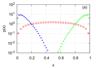
Figure 1: A comparison of a numerically calculated stationary PDF with no controlled agents, $M=M_{1}=0$ (red squares), and stationary PDF with controlled agents, $M=M_{1}=20$ (green circles) and $M=20$ and $M_{1}=0$ (blue triangles), in the non-extensive (a) and extensive (b) case. Model parameters were set as follows: $\sigma_{1}=\sigma_{2}=2$, $h=1$. A stochastic model, Eq. (8), was used for (a) and agent-based model, Eq. (7), with $N=10^{4}$ was used for (b).

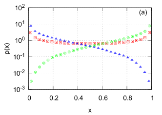
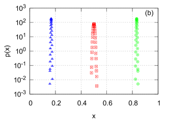
Figure 2: A comparison of a numerically calculated stationary PDF with no controlled agents, $M=M_{1}=0$ (red squares), and stationary PDF with controlled agents, $M=M_{1}=2$ (green circles) and $M=2$ and $M_{1}=0$ (blue triangles), in the non-extensive (a) and extensive (b) case. Model parameters were set as follows: $\sigma_{1}=\sigma_{2}=0.5$, $h=1$. A stochastic model, Eq. (8), was used for (a) and agent-based model, Eq. (7), with $N=10^{4}$ was used for (b).

In Fig. 1 we numerically confirm that a fixed small number of the controlled agents ($M=20$) enables us to significantly shift the stationary probability density function (abbr. PDF) of the macroscopic variable to the desired end despite the fact that the agents have strong individualistic tendencies, $\sigma_{i}>h$. If the agents have stronger herding behavior tendencies, $\sigma_{i}<h$, then the impact of the controlled agents is even stronger. In Fig. 2 we show that as few as two controlled agents are enough to significantly influence the stationary PDF of the model if herding behavior is prevalent.

An important question in this context is how fast the controlled agents are able to make the desired impact. Or namely, how fast the statistical properties of the system, PDF and mean, converge to the stationary ones. In case the other agents interact extensively the answer can be obtained analytically by solving corresponding ordinary differential equation, Eq. (9). Its solution is given by:

$$x(t)=x_{f}+[x(0)-x_{f}]\exp(-[hM+\sigma_{1}+\sigma_{2}]t),$$ (11)

here $x(0)$ is the initial condition and $x_{f}$ is a fixed point of Eq. (9), which is given by Eq. (10).

It is a more complex task to solve the non-extensive case, Eq. (8). One has to find the eigenvalues of the Fokker-Planck equation [37]. The problem is that the corresponding Fokker-Planck equation appears to be too complex to be dealt with analytically. A viable alternative, of course, is a numerical simulation. In Fig. 3 we plot the results of a numerical simulation, which show that the convergence times are finite for both mean and stationary PDF. Furthermore the obtained results show that the convergence of the mean is well described by the Eq. (11), and thus the convergence in both cases happen exponentially fast.

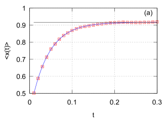
Figure 3: Time evolution of the mean (a) and the PDF (b) of $1000$ time series obtained by numerically solving the non-extensive stochastic model, Eq. (8). Subfigure (a): red squares represent the mean trajectory (average over ensemble of $1000$ realizations), blue curve is a plot of Eq. (11), while black curve represents the expected mean. Subfigure (b): different types of points represent PDF snapshots at distinct times (red squares - $t=0.05$, green circles - $t=0.1$, blue trinagles - $t=0.15$), gray curve represents the initial condition (the PDF at $t=0$), while black curve represents the expected PDF. Model parameters were set as follows: $\sigma_{1}=\sigma_{2}=2$, $h=1$, $M=M_{1}=20$.

4 Conclusions

In this contribution we have approached modeling of the control of collective behavior in complex socio-economic systems. Namely, we have modified a well-known agent-based herding model (originally introduced in [24]) to include agents, whose state is controlled exogenously. The control over a small number of the agents enabled us to significantly influence the behavior of the other agents, who act based on the rules of the original agent-based herding model. We found that even an infinitely large systems would be strongly affected, if the controlled agents interact with the other agents on the global scale (non-extensively). We find this to be in agreement with the related experiments [21, 22].

The control is even more effective if the other agents interact among themselves on the local scale (extensively). This may correspond to the actual dynamics of real societies, where most of the people interact in their “neighborhood“ (i.e. friends, coworkers and other acquaintances), while there are also some prominent individuals, leaders, who are able to influence the society on a global scale. Thus the mathematical model presented in this contribution may be also considered as a microscopic explanation of the leadership phenomenon in the contemporary society. The leadership, in this sense, can be seen as an exogenous information field in the similar way as parameters $\sigma_{i}$ can.

The ability to control the macroscopic dynamics of the agent-based herding model may allow future developments of the tools for preventing financial bubbles or crashes. It is thought that these extreme events may be caused by the herding behavior [38, 39], which is also the main ingredient of the model allowing control of the macroscopic dynamics. Furthermore the considered agent-based herding model was previously used to construct a simple agent-based models for the financial markets [17, 26, 27, 40]. In these models some of the states available to agents increase the market volatility (these states are related to the chartist trading strategies), while the others decrease (these states are related to the fundamentalist trading strategies). By using the results obtained in this contribution one could attract more agents to the lower volatility state thus decreasing volatility of the whole market.

References

- [1] M. Waldrop, Complexity: The emerging order at the edge of order and chaos, Simon and Schuster, New York, 1992.
- [2] G. Akerlof, J. Shiller, Animal Spirits: How Human Psychology Drives the Economy, and Why It Matters for Global Capitalism, Princeton University Press, 2009.
- [3] J. P. Bouchaud, Crises and collective socio-economic phenomena: Simple models and challenges, Journal of Statistical Physics 151 (2013) 567–606.
- [4] A. Kirman, Complex Economics: Individual and Collective Rationality, Routledge, 2010.
- [5] R. Axelrod, Advancing the art of simulation in the social sciences, Complexity 3 (1997) 16–32.
- [6] J. P. Bouchaud, Economics needs a scientific revolution, Nature 455 (2008) 1181.
- [7] R. Conte, N. Gilbert, G. Bonelli, C. Cioffi-Revilla, G. Deffuant, J. Kertesz, V. Loreto, S. Moat, J.-P. Nadal, A. Sanchez, A. Nowak, A. Flache, M. San Miguel, D. Helbing, Manifesto of computational social science, European Physics Journal Special Topics 214 (2012) 325–346.
- [8] M. Cristelli, L. Pietronero, A. Zaccaria, Critical overview of agent-based models for economics, in: F. Mallnace, H. E. Stanley (Eds.), Proceedings of the School of Physics ”E. Fermi”, Course CLXXVI, SIF-IOS, Bologna-Amsterdam, 2012, pp. 235 – 282.
- [9] J. D. Farmer, M. Gallegati, C. Hommes, A. Kirman, P. Ormerod, S. Cincotti, A. Sanchez, D. Helbing, A complex systems approach to constructing better models for managing financial markets and the economy, European Physics Journal Special Topics 214 (2012) 295–324.
- [10] S. Havlin, D. Y. Kenett, E. Ben-Jacob, A. Bunde, R. Cohen, H. Hermann, J. W. Kantelhardt, J. Kertesz, S. Kirkpatrick, J. Kurths, J. Portugali, S. Solomon, Challenges in network science: Applications to infrastructures, climate, social systems and economics, European Physics Journal Special Topics 214 (2012) 273–293.
- [11] V. Alfi, M. Cristelli, L. Pietronero, A. Zaccaria, Minimal agent based model for financial markets i: Origin and self-organization of stylized facts, European Physics Journal B 67 (2009) 385–397.
- [12] V. Alfi, M. Cristelli, L. Pietronero, A. Zaccaria, Minimal agent based model for financial markets ii: Statistical properties of the linear and multiplicative dynamics, European Physics Journal B 67 (2009) 399–417.
- [13] A. Chakraborti, I. M. Toke, M. Patriarca, F. Abergel, Econophysics review: Ii. agent-based models, Quantitative Finance 7 (2011) 1013–1041.
- [14] L. Feng, B. Li, B. Podobnik, T. Preis, H. E. Stanley, Linking agent-based models and stochastic models of financial markets, Proceedings of the National Academy of Sciences of the United States of America 22 (2012) 8388–8393.
- [15] R. Frederick, Agents of influence, Proceedings of the National Academy of Sciences of the United States of America 110 (2013) 3703–3705.
- [16] T. Kaizoji, Statistical properties of absolute log-returns and a stochastic model of stock markets with heterogeneous agents, Vol. 550 of Lecture Notes in Economics and Mathematical Systems, Springer-Verlag, 2005, pp. 237–248.
- [17] A. Kononovicius, V. Gontis, Agent based reasoning for the non-linear stochastic models of long-range memory, Physica A 391 (2012) 1309–1314.
- [18] R. Lye, J. P. L. Tan, S. A. Cheong, Understanding agent-based models of financial markets: A bottom up approach based on order parameters and phase diagrams, Physica A 391 (2012) 5521–5531.
- [19] T. Lux, M. Marchesi, Scaling and criticality in a stochastic multi-agent model of a financial market, Nature 397 (1999) 498–500.
- [20] J. Ruseckas, B. Kaulakys, V. Gontis, Herding model and 1/f noise, EPL 96 (2011) 60007.
- [21] J. R. G. Dyer, A. Johansson, D. Helbing, I. D. Couzin, J. Krause, Leadership, consensus decision making and collective behaviour in humans, Phylosophical Transactions of the Royal Society B 364 (2009) 781–789.
- [22] J. Krause, A. F. T. Winfield, J. L. Deneubourg, Interactive robots in experimental biology, Trends in Ecology and Evolution 26 (2011) 369–375.
- [23] F. Schweitzer, P. Mavrodiev, C. J. Tessone, How can social herding enhance cooperation?, CoRR (2012) abs/1211.1188.
- [24] A. P. Kirman, Ants, rationality and recruitment, Quarterly Journal of Economics 108 (1993) 137–156.
- [25] C. Castellano, S. Fortunato, V. Loreto, Statistical physics of social dynamics, Reviews of Modern Physics 81 (2009) 591–646.
- [26] S. Alfarano, T. Lux, F. Wagner, Estimation of agent-based models: The case of an asymmetric herding model, Computational Economics 26 (2005) 19–49.
- [27] S. Alfarano, T. Lux, F. Wagner, Time variation of higher moments in a financial market with heterogeneous agents: An analytical approach, Journal of Economic Dynamics and Control 32 (2008) 101–136.
- [28] J. M. Pasteels, J. L. Deneubourg, S. Goss, Self-organization mechanisms in ant societies (i): Trail recruitment to newly discovered food sources, in: J. M. Pasteels, J. L. Deneubourg (Eds.), From Individual to Collective Behaviour in Social Insects, Birkhauser, Basel, 1987, pp. 155–175.
- [29] J. M. Pasteels, J. L. Deneubourg, S. Goss, Self-organization mechanisms in ant societies (ii): Learning in foraging and division of labor, in: J. M. Pasteels, J. L. Deneubourg (Eds.), From Individual to Collective Behaviour in Social Insects, Birkhauser, Basel, 1987, pp. 177–196.
- [30] G. S. Becker, A note on restaurant pricing and other examples of social influence on price, Journal of Political Economy 99 (1991) 1109–1116.
- [31] M. Aoki, H. Yoshikawa, Reconstructing Macroeconomics: A Perspektive from Statistical Physics and Combinatorial Stochastic Processes, Cambridge University Press, 2007.
- [32] S. Alfarano, M. Milakovic, Network structure and n-dependence in agent-based herding models, Journal of Economic Dynamics and Control 33 (2009) 78–92.
- [33] A. Traulsen, J. C. Claussen, C. Hauert, Stochastic differential equations for evolutionary dynamics with demographic noise and mutations, Physical Review E 85 (2012) 041901.
- [34] S. Alfarano, M. Milakovic, M. Raddant, A note on institutional hierarchy and volatility in financial markets, The European Journal of Finance 19 (2013) 449–465.
- [35] A. Carro, R. Toral, M. San Miguel, Signal amplification in an agent-based herding model (2013).
- [36] C. W. Gardiner, Handbook of stochastic methods, Springer, Berlin, 2009.
- [37] H. Risken, The Fokker-Planck Equation: Methods of Solutions and Applications, 3rd Edition, Springer, 1996.
- [38] T. Preis, D. Y. Kenett, H. E. Stanley, D. Helbing, E. Ben-Jacob, Quantifying the behavior of stock correlations under market stress, Scientific Reports 2 (2012) 752.
- [39] D. R. Parisi, D. Sornette, D. Helbing, Financial price dynamics and pedestrian counterflows: A comparison of statistical stylized facts, Physical Review E 87 (2013) 012804.
- [40] A. Kononovicius, V. Gontis, Three state herding model of the financial markets, EPL 101 (2013) 28001.