Quasi-Periodic Oscillations and energy spectra from the two brightest Ultra-Luminous X-ray sources in M 82

Abstract

Ultra-Luminous X-ray sources are thought to be accreting black holes that might host Intermediate Mass Black Holes (IMBH), proposed to exist by theoretical studies, even though a firm detection (as a class) is still missing. The brightest ULX in M 82 (M 82 X–1) is probably one of the best candidates to host an IMBH. In this work we analyzed the data of the recent release of observations obtained from M 82 X–1 taken by XMM-Newton. We performed a study of the timing and spectral properties of the source. We report on the detection of ${\approx}(46{\pm}2)$ mHz Quasi-Periodic Oscillations (QPOs) in the power density spectra of two observations. A comparison of the frequency of these high-frequency QPOs with previous detections supports the 1:2:3 frequency distribution as suggested in other studies. We discuss the implications if the ${\approx}(46{\pm}2)$ mHz QPO detected in M 82 X–1 is the fundamental harmonic, in analogy with the High-Frequency QPOs observed in black hole binaries. For one of the observations we have detected for the first time a QPO at 8 mHz (albeit at a low significance), that coincides with a hardening of the spectrum. We suggest that the QPO is a milli-hertz QPO originating from the close-by transient ULX M 82 X–2, with analogies to the Low-Frequency QPOs observed in black hole binaries.

1 Introduction

Ultra-Luminous X-ray sources (ULXs) are point-like, off-nuclear, extra-galactic sources, with observed X-ray luminosities (${\rm L}_{\rm X}{\geq}10^{39}\,{\rm erg}\,{\rm s}^{-1}$) higher than the Eddington luminosity for a stellar-mass black-hole (${\rm L}_{\rm X}{\approx}10^{38}\,{\rm erg}\,{\rm s}^{-1}$). The true nature of these objects is still debated (Feng & Soria, 2011; Fender & Belloni, 2012). Although the definition of ULXs encompasses different types of sources, the majority of them are likely to be accreting BHs in binary systems. However, there is still no unambiguous estimate for the mass of the compact object hosted in these systems. Assuming an isotropic emission, in order to avoid the violation of the Eddington limit, ULXs might be powered by accretion onto Intermediate Mass Black Holes (IMBHs) with masses in the range $10^{2}-10^{4}\,{\rm M}_{\odot}$ (Colbert & Mushotzky, 1999). It has been also suggested that ULXs appear very luminous because of beaming (King et al., 2001), super-Eddington emission (Begelman, 2002), a combination of these effects (Poutanen et al., 2007) or because they contain a moderately high mass BH (Zampieri & Roberts 2009; Mapelli et al. 2009).

An approach to study the nature of ULXs is through time variability. The analysis of the aperiodic variability in the X-ray flux of X-ray binaries is a powerful tool to study the properties of the inner regions of the accretion disc around compact objects (for a review see van der Klis 2005). In particular, Quasi-Periodic Oscillations (QPOs) provide well-defined frequencies, which can be linked to specific time scales in the disc. QPOs in Black Hole Binaries (BHBs) can be broadly divided into three classes: (i) QPOs at very low frequencies ($<0.02$ Hz), probably associated to oscillations and instabilities in the accretion disc (see Morgan et al. 1997; Belloni et al. 1997, 2000); (ii) Low-Frequency QPOs (LFQPOs), with typical frequencies between 0.1 and 10 Hz, probably connected to similar oscillations in neutron star systems (see e.g. Belloni et al. 2002; Remillard et al. 2002a; van der Klis 2005; Casella, Belloni & Stella 2005), over whose origin there is no consensus; in Black Hole Binaries (BHBs) 3 main different types of LFQPOs have been identified (Casella, Belloni & Stella 2005, and references therein); (iii) High-Frequency QPOs (HFQPOs), with a typical frequency of ${\approx}35-450$ Hz, in a few cases observed to appear in pairs (Strohmayer, 2001a, b; Belloni et al., 2012, 2013). It is currently unclear whether these QPOs have constant frequencies and whether they have special ratios (Belloni et al., 2013). However, since they identify the highest frequencies observed in these systems, they are the best candidates for association with, e.g., the Keplerian frequency at the innermost stable orbit. Whatever their physical nature, as they originate in the inner regions of accretion discs around black holes, these features are expected to be produced also in ULXs. However, if ULXs contain IMBHs of $(10^{2}-10^{4})\,{\rm M}_{\odot}$, the frequencies are correspondingly smaller.

In this paper we report on the results from a joint spectral and timing analysis of five $20-30$ ks XMM-Newton observations of M 82 performed on March-November 2011. The plan of the paper is the following. In Sec. 2, 3 we present the timing and spectral analysis of the data. Sec. 4 reports the detection of QPOs in the data, together with a comparison with previous findings. The results from the spectral analysis and the relationship with the timing properties are also shown. Finally, in Sec. 5 we discuss our results.

1.1 M 82 X–1

M 82 X–1 (also named CXOU J095550.2+694047) is one of the brightest ULXs in the sky. Its host galaxy is the prototype of starburst galaxy and is located nearby, at a distance of 3.9 Mpc (Sakai & Madore, 1999), making M 82 X–1, with an average X-ray luminosity ${\gtrsim}10^{40}$ ${\rm erg\,s^{-1}}$, an excellent target for performing X-ray studies. The position of M 82 X–1 is within $1\arcsec$ of the position of the infrared source and super star cluster MGG 11 (Kaaret et al., 2004; Portegies Zwart et al., 2004). Simulations of the dynamical evolution of the cluster MGG 11 show that stellar collisions in its extremely dense core may have led to the formation of an IMBH (Portegies Zwart et al., 2004). Strohmayer & Mushotzky (2003) found QPOs in the range 50–110 mHz which they identified as arising from M 82 X–1 (and later confirmed by Feng & Kaaret 2007 using Chandra data). If the QPO frequency is associated with the orbital frequency around a non-rotating black hole, then it would imply a mass limit of $2{\times}10^{4}\,{\rm M}_{\odot}$. The QPOs were discovered in XMM-Newton data and confirmed in RXTE data (Strohmayer & Mushotzky, 2003). The QPOs are only occasionally detected in the RXTE data and no apparent correlation between QPO detections and the source flux level has been found. Based on a comparison of the spectral and timing properties of stellar-mass black hole X-ray binaries, Fiorito & Titarchuk (2004) estimated a mass of the order of $10^{3}{\rm M}_{\odot}$ for the compact object producing the QPOs. The method uses the photon index-QPO frequency correlation that has been seen in BHBs (Vignarca et al., 2003; Titarchuk & Fiorito, 2004). The QPOs were confirmed in a longer XMM-Newton observation, where their frequency was 113 mHz (Mucciarelli et al., 2006; Dewangan et al., 2006). Also Casella et al. (2008) estimated the mass of the BH to be in the range $(100-10^{3}){\rm M}_{\odot}$. Their method relies in the location of the ULX in the variability plane of BHs, that relates the mass of the BH with its timing properties.

1.2 M 82 X–2

The X-ray source M 82 X–2 (also named CXOU J095551.4+694043) was identified as a transient ULX in M 82 from multiple X-ray observations with Chandra (Kaaret et al., 2006; Feng & Kaaret, 2007; Kong et al., 2007). It lies on the sky plane at $5^{\prime\prime}$ from M 82 X–1, which is most of the time the brightest source in M82. Only Chandra is able to resolve them in X-rays. From Chandra observations it has been seen that M 82 X–2 is sometimes the second brightest X-ray source in M 82, but it is undetected during the rest of the time (Matsumoto et al., 2001; Feng & Kaaret, 2007). Feng & Kaaret (2007) argued that M 82 X–2 is more likely to be an IMBH than a stellar-mass object accreting from a massive star according to its transient nature and high outburst-luminosity (${\approx}10^{40}$ ${\rm erg\,s^{-1}}$; Kalogera et al. 2004). Kaaret et al. (2006) reported significant timing noise near 1 mHz from M 82 X–2 in one Chandra observation that later Feng et al. (2010) confirmed it in the form of a milli-hertz QPO. Identifying the frequency of this QPO to that of a LFQPO and applying a linear mass-frequency scaling relationship Feng et al. (2010) derived a value of ${\approx}10^{4}{\rm M}_{\odot}$ for the mass of the BH.

2 Observations and data reduction

In this work we analyzed the recently publicly available observations of M 82 X–1 collected by the XMM-Newton satellite (see Tab. 1 for details). The EPIC camera was operating in the Full Frame mode and with the Medium Filter set.

For the timing analysis, we filtered the EPIC pn+MOS event files, selecting only the best-calibrated events (pattern${\leq}4,12$ for the pn and the MOS, respectively), and rejecting flagged events (i.e. keeping only flag$=0$ events) from a circular region on the source (centre at coordinates ${\rm RA}=09\,h55\,m50.2\,s$, ${\rm Dec}=+69\,d40\,m47\,s$; Mucciarelli et al. 2006) and radius $13\,$arcsec. Many gaps in the light curves were present. These gaps are of instrumental origin, due to periods of intense background flaring. How we dealt in the analysis with these time periods is shown in Sec. 3.1. No background subtraction was applied, to preserve the statistical properties of the distribution of powers in the power spectrum. We payed particular attention to extract the list of photons not randomized in time. To this purpose, we used the tasks epchain for the pn and emproc (with randomizetime=no) for the MOS cameras, respectively.

For the spectral analysis we used only the EPIC pn camera, in order to avoid issues due to cross-calibration effects. Additionally, the EPIC pn camera has a higher effective area (i.e. double) than each one of the MOS cameras and has sufficient statistics for the fit. We applied the standard filtering of removing time periods with high count-rates in the FOV in the 10-12 keV energy range (EPIC-pn only). We filtered the event files, selecting only the best-calibrated events (pattern${\leq}4$ for the pn), and rejecting flagged events (flag$=0$). We extracted the flux from a circular region on the source centred at the coordinates of the source and radius $13\,$arcsec (the same as the region used for the timing analysis). The background was extracted from a circular region (with a radius of $18\,$arcsec), centred in a position in the same chip, far away from the boundaries and not far from the source. We built response functions with the Science Analysis System (SAS) tasks rmfgen and arfgen. We fitted the background-subtracted spectra with standard spectral models in XSPEC 12.7.0 (Arnaud, 1996). All errors quoted in this work are $68\%$ ($1{\sigma}$) confidence. The spectral fits were limited to the 0.3-10 keV range, where the calibration of the instruments is the best. The spectra were rebinned in order to have at least 25 counts for each background-subtracted spectral channel and to avoid oversampling of the intrinsic energy resolution by a factor larger than 3 .

Table 1: Log of the observations from this work.

Obs. Number	Obs. Date	MJD	Exposure Time 1 (seconds)
1	2011–03–18	55 638	26 657
2	2011–04–09	55 660	23 836
3	2011–04–29	55 680	28 219
4	2011–09–24	55 828	22 843
5	2011–11–21	55 886	23 914

3 Analysis

3.1 Timing Analysis

We performed an analysis of the fast time variability of M 82 X–1 in the 1-10 keV energy range. The (0.3-1 keV) and (1-10 keV) EPIC non-background subtracted count rates are ${\approx}0.20\,{\rm cts}\,{\rm s}^{-1}$ and $(1-2)\,{\rm cts}\,{\rm s}^{-1}$, respectively. Since the (0.3-1 keV) count rate is very low we ignored this energy range in the analysis and limited it to the (1-10 keV) energy range since it has better statistics. The time resolution of the instruments is 2.6 s (MOS) and 73.4 ms (pn).

The pn+MOS light curve was binned at the lowest time resolution of the two (2.6 s). This yields a Nyquist frequency of $=0.19$ Hz. We produced Power Density Spectra (PDS) using intervals of 512 bins in each light curve. The PDS were then averaged together for each observation. Many gaps (153 and 56 with a duration of ${\leq}100$ s each, which represent ${\approx}50,25\%$ of the total time of the light curves, respectively) were present in the light curves of Obs. 2, 3 and were filled with a Poissonian realization around the local mean value of counts before and after the gap. The PDS were normalized according to Leahy et al. (1983). The resulting total PDS was logarithmically rebinned with the bin increase with frequency adjusted on a case by case basis, in order to improve the statistics. All of the PDS show low-frequency flat-topped noise.

PDS fitting was carried out with the standard XSPEC fitting package by using a unit response. Fitting the (1-10 keV) PDS with a model composed by a Lorentzian for the low-frequency noise and a constant for the Poisson noise results in non acceptable chi-square values (${\chi}^{2}/{\nu}=87/61,143/100,170/100,57/41$) for Obs. 1-4. The width and the fractional rms of the zero-centred Lorentzian component are $(3-70)$ mHz and $(10-18)\%$ for Obs. 1-4, respectively. In the case of Obs. 5 this model is a good description of the data (${\chi}^{2}/{\nu}=101/100$). The width and the fractional rms of the zero-centred Lorentzian component are $1.3_{-0.8}^{+2.0}$ mHz and $(11.8{\pm}1.4)\%$ in this observation. The PDS of Obs. 3 shows positive residuals at low-frequencies that we fitted with an additional power-law component, yielding an improvement of the fit of ${\Delta}{\chi}^{2}=20$ for ${\nu}=2$.

With the continuum model adopted, the (1-10 keV) PDS of Obs. 1-4 still show positive residuals centred at ${\nu}_{\rm QPO}{\approx}50,8,40,30\,{\rm mHz}$. We added a Lorentzian component to fit these excesses. The detection of this peak is significant (${\geq}3.6{\sigma}$, calculated as the value of the Lorentzian normalization divided by its $1{\sigma}$ error) except for Obs. 4 ($<3{\sigma}$). The integrated 1-10 keV fractional variability of these QPOs are ${\approx}8-10\%$. The final fits result in mostly acceptable chi-square values ${\chi}^{2}/{\nu}=61/58,127/97,119/95,43/38,101/100$ for Obs. 1-5, respectively. The PDS are plotted in Fig. 1 and the parameters from the fits and the QPOs obtained are in Tab. 2 .

Figure 1: Power density spectra from the XMM-Newton EPIC/pn data used in this work in the (1–10 keV) energy band and $(4{\times}10^{-4}-0.2)$ Hz frequency range during observations 1–5 (top-left to bottom-right) with the best fit model (solid line) and the model components (dotted line).

Table 2: Values obtained from the timing analysis.

	Obs. 1	Obs. 2	Obs. 3	Obs. 4	Obs. 5
Count rate 1 (${\rm cts}\,{\rm s}^{-1}$)	$2.39{\pm}0.02$	$2.77{\pm}0.02$	$2.10{\pm}0.02$	$2.33{\pm}0.02$	$3.15{\pm}0.02$
${\nu}_{\rm lor}$ (mHz)	$0$	$0$	$0$	$0$	$0$
FWHM (mHz)	$50{\pm}20$	$3.3{\pm}0.6$	$60{\pm}20$	$70{\pm}20$	$1.3_{-0.8}^{+2.0}$
Norm.	$0.06{\pm}0.03$	$0.21{\pm}0.03$	$0.06{\pm}0.02$	$0.13{\pm}0.04$	$0.13_{-0.06}^{+0.14}$
Fractional rms ($\%$)	$10.5{\pm}1.4$	$17.8{\pm}1.2$	$11.8{\pm}1.6$	$15.4{\pm}0.9$	$11.8{\pm}1.4$
${\nu}_{\rm QPO}$ (mHz)	$48.1{\pm}1.1$	$8.3{\pm}0.2$	$44.1{\pm}0.5$	$35.2{\pm}1.2$	–
${\rm FWHM}$ (mHz)	$9{\pm}4$	$0.9{\pm}0.4$	$4{\pm}2$	$7{\pm}4$	–
${\rm Norm.}$	$0.026{\pm}0.007$	$0.016{\pm}0.004$	$0.016{\pm}0.004$	$0.015{\pm}0.006$	–
Fractional rms ($\%$)	$10.2{\pm}1.4$	$7.6{\pm}0.9$	$9{\pm}2$	$8.0{\pm}1.8$	–
${\rm Significance}_{\rm QPO}$ (${\sigma}$) 2	$3.6$	$3.8$	$4.5$	$2.6$	–
${\Gamma}_{\rm poisson}$	$0$	$0$	$0$	$0$	$0$
${\rm Norm.}_{\rm poisson}$	$1.93{\pm}0.07$	$1.93{\pm}0.03$	$1.92{\pm}0.06$	$1.78{\pm}0.10$	$2.05{\pm}0.03$
${\Gamma}$	–	–	$2.3{\pm}0.4$	–	–
Norm.	–	–	${\leq}10^{-6}$	–	–
${\chi}^{2}/{\nu}$	$61/58$	$127/97$	$119/95$	$43/38$	$101/100$

3.2 Spectral Analysis

We started fitting the spectra with an absorbed power-law model, using the Tuebingen-Boulder ISM absorption model (tbabs in XSPEC) to account for the interstellar absorption (${\rm N}_{\rm H}=4{\times}10^{20}\,{\rm cm}^{-2}$ in the direction to M 82). This parameter was set free to vary in order to account for intrinsic absorption. We fitted the spectra simultaneously, constraining the column density to be the same for all the spectra. With this model we obtained a bad description of the spectra (${\chi}^{2}/{\nu}{\gg}2$ with ${\nu}=781$ d.o.f.), with positive residuals at ${\leq}2$ keV and high-energy curvature at ${\gtrsim}5$ keV. The spectra are curved with a break at ${\approx}5-7$ keV, in agreement with what has been found in previous studies from a sample of ULXs (see e.g. Stobbart et al. 2006; Gladstone et al. 2009; Caballero-Garcia & Fabian 2010; Caballero-Garcia 2011).

To account for the low-energy residuals, that are in the form of excesses at low energies (around 1 and 2 keV) we had to include an apec model, which accounts for the diffuse X-ray emission from the galaxy. We fixed the metal abundances to solar, in agreement with a previous work based on XMM-Newton data (Read & Stevens, 2002). We obtained a better fit (${\chi}^{2}/{\nu}{\approx}2.0$, with ${\nu}=779$). Some residuals in the form of excesses at around 2 keV were still present. In a different context, Stevens et al. (2003) tried to fit the nuclear emission of M 82 with two components coming from the diffuse emission of the galaxy. Therefore, we included a second apec model but this was not enough to improve neither the spectral fit (${\chi}^{2}/{\nu}{\approx}2.0$, with ${\nu}=782$) nor the appearance of the residuals. The parameters of the apec components were constrained to be the same between the observations. Following Stevens et al. (2003); Mucciarelli et al. (2006); Ranalli et al. (2008) we tried to fit the residual galactic emission with a dual apec model with different absorbing columns. That improved the fit (${\Delta}{\chi}^{2}{\approx}390$ for 3 d.o.f.) and flattened the low-energy residuals. Nevertheless, the fit was still poor (${\chi}^{2}/{\nu}=1.9$ with ${\nu}=775$). The column densities obtained are in agreement with those obtained from Chandra observations at the position of the ULX (Feng & Kaaret, 2010).

To account for the high-energy residuals we added a cut-off, replacing the power-law component by a high-energy cut-off (highecut*powerlaw in XSPEC) model to fit the high-energy spectra. This model improved the fit substantially (${\chi}^{2}/{\nu}=1.16$, with ${\nu}=765$). We included a multicolor inner disc emission component (diskbb in XSPEC), as previously done by Mucciarelli et al. (2006). This improved the fit statistics by ${\Delta}{\chi}^{2}=43$ for ${\nu}=10$ d.o.f. (i.e. a $4{\sigma}$ improvement). We also tried by substituting the cut-off power-law by the more physical compTT model. The temperature for the input photons from the Comptonization component was set equal to the inner disc temperature. We also tried to fit the spectra not fixing the inner disc temperature to the temperature of the input photons from the Comptonization component and obtained a non-significant improvement of the fit (i.e. $<3{\sigma}$). Therefore we kept the constraint. With this model we obtained very similar quality of the fits (${\chi}^{2}/{\nu}{\approx}1.15$, with ${\nu}=760$). The improvement of the fit by adding the disc component (diskbb in XSPEC) was found to be significant at the $3.6{\sigma}$ level. The resulting parameters are in agreement with previous studies for a sample of ULXs (Gladstone et al., 2009).

The most relevant results of this spectral analysis and the derived unabsorbed fluxes are in Tab. 3 and in Fig. 2. The errors on the total flux (plus the flux from every individual component) were calculated with the cflux command in XSPEC. We have to notice that, because XMM-Newton is unable to resolve M 81 X–1 from M 82 X–2, great caution is needed in order to interpret the results obtained from the spectral analysis. We find very low values for the photon indices from the high-energy power-law (${\Gamma}=0.6-1.1$). These values are much lower than those typically seen in the high-energy spectra from ULXs (${\Gamma}=1.5-2.5$) and might be a consequence of the fact that there is a large overlap between the Point Spread Functions (PSD) from M 82 X–1 and M 82 X–2 with XMM-Newton. Indeed, in studies of the Chandra spectra, it has been found that the best description of the spectrum from M 82 X–2 is composed by multi-color disc plus power-law high-energy emission, the last with a very flat photon index, i.e. ${\Gamma}=1.19{\pm}0.06$. This prevents us from making a quantitative comparison of the photon index/flux from the high-energy emission versus the frequency of the QPO, as in the relationships typically seen in stellar-mass BHBs (Vignarca et al., 2003; Titarchuk & Fiorito, 2004). The summed total (0.3-10 keV) unabsorbed fluxes observed are in the range $(3.4-4.3){\times}10^{-11}\,{\rm erg}{\rm s}^{-1}{\rm cm}^{-2}$, consistently with what has been found previously (Mucciarelli et al., 2006). In the case of Obs. 2, 5 we see an increase in the total flux, that is accompanied by a strong flattening of the spectra. This might indicate that in Obs. 2, 5 the contribution to the total flux from M 82 X–2 is important.

Table 3: Results obtained from the spectral analysis.

Spectral parameter 1	Obs. 1 (Black)	Obs. 2 (Red)	Obs. 3 (Green)	Obs. 4 (Dark Blue)	Obs. 5 (Light Blue)
			A
${\rm N}_{\rm H}$(1) $({\times}10^{22})\,({\rm cm}^{-2})$	$0.075{\pm}0.003$	$=$	$=$	$=$	$=$
${\rm kT}_{1}$ (keV)	$0.75{\pm}0.02$	$=$	$=$	$=$	$=$
${\rm N}_{\rm H}$(2) $({\times}10^{22})\,({\rm cm}^{-2})$	$1.39{\pm}0.02$	$=$	$=$	$=$	$=$
${\rm kT}_{2}$ (keV)	$0.91{\pm}0.02$	$=$	$=$	$=$	$=$
${\rm N}_{\rm H}$(3) $({\times}10^{22})\,({\rm cm}^{-2})$	$0.756{\pm}0.007$	$=$	$=$	$=$	$=$
${\rm kT}_{\rm max}$ (keV)	$0.18{\pm}0.17$	$0.29{\pm}0.05$	$0.19{\pm}0.02$	$0.16{\pm}0.02$	$0.26{\pm}0.02$
${\rm N}_{\rm disc}$	$70{\pm}23$	$2.8{\pm}1.9$	$240_{-150}^{+230}$	$540{\pm}70$	$42{\pm}20$
${\rm E}_{\rm c}$ (keV)	$5.38{\pm}0.10$	$4.49{\pm}0.10$	$6.75{\pm}0.12$	$6.22{\pm}0.12$	$6.04{\pm}0.10$
${\rm E}_{\rm f}$ (keV)	$5.8{\pm}0.6$	$5.4{\pm}0.4$	$4.6{\pm}0.7$	$4.5{\pm}0.8$	$5.6{\pm}0.7$
${\Gamma}$	$0.86{\pm}0.02$	$0.60{\pm}0.02$	$1.13{\pm}0.02$	$1.06{\pm}0.02$	$0.71{\pm}0.02$
${\chi}^{2}/{\nu}=849/755$
${\rm F}_{\rm pow}$ 2 (1-10 keV)	$1.27{\pm}0.06$	$1.58{\pm}0.08$	$0.93{\pm}0.05$	$1.17{\pm}0.06$	$1.89{\pm}0.10$
			B
${\rm N}_{\rm H}$(1) $({\times}10^{22})\,({\rm cm}^{-2})$	$0.09{\pm}0.02$	$=$	$=$	$=$	$=$
${\rm kT}_{1}$ (keV)	$0.76{\pm}0.02$	$=$	$=$	$=$	$=$
${\rm N}_{\rm H}$(2) $({\times}10^{22})\,({\rm cm}^{-2})$	$1.47{\pm}0.02$	$=$	$=$	$=$	$=$
${\rm kT}_{2}$ (keV)	$0.92{\pm}0.02$	$=$	$=$	$=$	$=$
${\rm N}_{\rm H}$(3) $({\times}10^{22})\,({\rm cm}^{-2})$	$0.84{\pm}0.02$	$=$	$=$	$=$	$=$
${\rm kT}_{\rm max}$ (keV)	$0.16{\pm}0.02$	$0.11{\pm}0.02$	$0.17{\pm}2$	$0.15{\pm}0.02$	$0.23{\pm}0.02$
${\rm N}_{\rm disc}$	$500^{+600}_{-300}$	$1\,600{\pm}1\,500$	$690{\pm}120$	$1\,100{\pm}500$	$100^{+60}_{-40}$
${\rm kT}_{\rm e}$ (keV)	${\leq}2$	${\leq}2$	$2.12{\pm}0.02$	${\leq}2$	$2.18{\pm}0.06$
${\tau}$	$14.2{\pm}0.2$	$16.00{\pm}0.17$	$11.9{\pm}.5$	$12.8{\pm}0.2$	$15.1{\pm}0.7$
${\chi}^{2}/{\nu}=872/760$
${\rm F}_{\rm compTT}$ 2 (1-10 keV)	$1.25{\pm}0.06$	$1.66{\pm}0.08$	$0.92{\pm}0.05$	$1.18{\pm}0.06$	$1.89{\pm}0.09$
${\rm L}_{\rm X,compTT}$ (0.3-10 keV)	$2.45{\pm}0.13$	$3.21{\pm}0.16$	$1.83{\pm}0.98$	$2.35{\pm}0.11$	$3.60{\pm}0.18$

4 Results

In Fig. 1 we show the (1-10 keV) PDS from the most recent set of 5 observations of the central region of M 82 performed with XMM-Newton. QPOs are seen in the PDS of Obs. 1–4 at frequencies ${\nu}=(48.1{\pm}1.1,8.3{\pm}0.2,44.1{\pm}0.5,35.2{\pm}1.2)$ mHz, respectively. The best-fit parameters for the QPOs found are shown in Tab. 2. The detection significance of the QPOs of Obs. 1–3 is ${\geq}3.6{\sigma}$ (single trial) but the QPO of Obs. 4 is not significant. We have calculated the chance probability of getting these peaks by taking into account the total number of trials and found them to be $8.7{\times}10^{-3},3.9{\times}10^{-2},4.2{\times}10^{-4}$ for Obs. 1, 2, 3, respectively. In order to estimate the number of trials for our detections we multiplied the number of observations analyzed, five, by the number of independent frequencies sampled. For the latter, we considered that we would have accepted QPOs in the range $0.01-1$ Hz, and for each observation divided that range by the FWHM of the detected QPO. Therefore, after considering the number of trials, only the QPOs at Obs. 1, 3 are significant detections (${\approx}3{\sigma}$, after considering all the trials), whilst the QPO at Obs. 2 is detected only marginally (${\approx}2{\sigma}$). The frequency from the QPOs at Obs.1, 3 differ by ${\Delta}=4{\pm}1.2$ mHz and have a mean value of 46 mHz. Although the difference between the two frequencies is statistically different from zero at the $3\,{\sigma}$ level. we will refer in the following to the QPOs from Obs. 1, 3 as the same one with a frequency equal to their mean value. The frequency of the QPO of Obs. 2 has much a lower frequency (${\nu}=8.3{\pm}0.2$ mHz).

We compared the QPOs found in our work with all those QPOs from M 82 X–1 that have been detected in the literature so far (see list in Tab. 4). The QPOs we have found at ${\nu}\approx 46$ mHz have roughly similar frequencies to the QPOs detected at ${\nu}{\approx}(50-70)$ mHz by Mucciarelli et al. (2006). On the other hand, the QPO we have detected at $(8.3{\pm}0.2)$ mHz has never seen before in M 82 X–1. In Fig. 3 we plot the time history of the centroid frequencies of all the QPOs detected from M 82 X–1 from all X-ray satellites (i.e. XMM-Newton, Chandra and RXTE) so far. QPOs marked with dot-filled circles were reported as ${\approx}4{\sigma}$ detections with RXTE by Kaaret et al. (2006). The QPOs reported by Kaaret et al. (2006) appear to be single trial and no significances were given observation by observation. To include them in our comparison we extracted the same observations and applied the same analysis as described in their paper, fitting the PDS and obtaining single-trial significances. We then derived final chance probabilities by estimating the number of trials as we had done for our detections. We obtained that the chance probabilities of detection of their QPOs are in the range $0.268-0.873$ except for the QPOs at ($103{\pm}5,83{\pm}5$) mHz during MJD=53 334,53 098, for which we have found chance probabilities of $3.9{\times}10^{-2},6.31{\times}10^{-3}$. Therefore, applying the same significance criteria that we used for our observations, we only consider that the QPO at $(83{\pm}5)$ mHz from Kaaret et al. (2006) is significant (${\approx}3{\sigma}$, after considering all the trials) whilst the QPO at $103{\pm}5$ mHz is marginally significant (${\approx}2{\sigma}$) . The second one is very similar to the QPO found previously from M 82 X–1 (Strohmayer & Mushotzky, 2003; Fiorito & Titarchuk, 2004; Mucciarelli et al., 2006). Nevertheless, a similar QPO to the first one, centred at ${\approx}70$ mHz has been tentatively detected previously in a Chandra PDS of M 82 X–2 (Kaaret et al., 2006). Taking these considerations into account and looking only at the significant detections from M 82 X–1 (i.e. looking at the solid-filled circles from Fig. 3 only) we see a rough 1:2:3 distribution in frequency of the QPOs, compatible with the QPO at ${\nu}{\approx}50$ mHz being the fundamental one. In Fig. 3 we plot the distribution on time of the detections, from which the 1:2:3 distribution of the frequencies of the QPOs in M 82 X–1 is clearly seen.

In Fig. 2 we plot all our spectra from XMM-Newton. Considering the most physical model (i.e. model B in Tab. 3) we see a change in the flux from the high-energy component. The flux variations of the high-energy component from M 82 X–1 in Obs.1–4 are $>3{\sigma}$ with respect to the mean value. We plotted the flux from the high-energy component versus the frequency of the QPO (see Fig. 4). We can see that the appearance of a lower-frequency QPO coincides with an increase of the flux from the high-energy component, i.e. a hardening of the spectrum. We discussed in Sec. 3.2 that this hardening is probably due to an increased flux from the nearby ULX M 82 X–2.

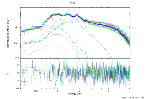
Figure 2: Energy spectra from M 82 during Obs 1–5 (black, red, green, dark and light blue, respectively).

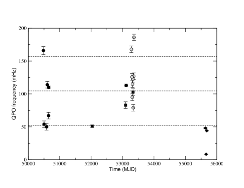
Figure 3: Time history of the centroid frequencies of the QPOs from M 82 with significance (${\sigma}>3$, single trial) from the total sample (see Tab. 4). The QPOs from our work and from Mucciarelli et al. (2006); Strohmayer & Mushotzky (2003) are indicated with solid diamonds/circles/squares, respectively and the QPOs from Kaaret et al. (2006) are indicated with dotted-filled circles/squares for the non-significant/significant detections, after taking into account all the trials. Dashed lines mark the frequencies ${\nu}=(52.3,2{\times}52.3,3{\times}52.3)$ mHz, in which ${\nu}=52.3$ mHz is the mean value of the frequencies from Tab. 4 in the range $(44-67)$ mHz.

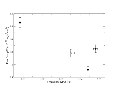
Figure 4: Unabsorbed flux from the high-energy component versus the frequency of the QPOs from our work (both in the 1-10 keV energy range) detected with significance ${\geq}3.6{\sigma}$ (solid-filled circles). The QPO at ${\approx}30$ mHz detected in our work with significance $<3{\sigma}$ has also been plotted (dot-filled circle).

Table 4: List of all the QPOs from M 82 detected in the literature.

Date	MJD	QPO ${\nu}$ (mHz)	${\rm n}_{\sigma}$	Ref. 1
1997 Feb 02	50 481	166$\pm$6	6.8	1
1997 Feb 24	50 503	54$\pm$5	5.3	1
1997 May 16	50 584	50$\pm$5	6.0	1
1997 Jun 07	50 606	114$\pm$5	5.8	1
1997 Jul 16	50 645	67$\pm$5	6.5	1
1997 Jul 21	50 650	110$\pm$2	4.3	1
2004 Apr 21	53 116	113$\pm$2	8.9	1
2001 May 06	52 035	51$\pm$2	8.0	2
2004 Dec 25	53 364	186$\pm$5	4.0	3
2004 Dec 17	53 356	127$\pm$5	4.0	3
2004 Dec 01	53 340	79$\pm$5	4.0	3
2004 Nov 25	53 334	103$\pm$5	4.0	3
2004 Nov 19	53 328	123$\pm$5	4.0	3
2004 Nov 09	53 318	115$\pm$5	4.0	3
2004 Nov 01	53 310	95$\pm$5	4.0	3
2004 Oct 24	53 302	126$\pm$5	4.0	3
2004 Oct 04	53 282	168$\pm$5	4.0	3
2004 Apr 03	53 098	83$\pm$5	4.0	3

5 Discussion

In this work we report on the finding of two QPOs at a mean frequency value of ${\approx}46$ mHz in the observations of the Ultra-Luminous X-ray source M 82 X–1. The XMM-Newton observations have been performed in the time interval of ${\approx}250$ days, over which we detected (at different significance levels) QPOs with different frequencies, i.e. a QPO at 46 mHz in Obs. 1, 3, and a QPO at 8 mHz during Obs. 2. These three observations have been performed in the time interval of only ${\approx}50$ days, indicating the fast variability in this source can change on a scale of only a few weeks. For Obs. 4, 5 we do not detect any significant QPO (we obtained $3{\sigma}$ upper limits of $5\%$ for the fractional rms of a QPO at ${\approx}46$ mHz for these observations). Additionally, we find that the QPO frequencies are roughly consistent with being anti-correlated with the flux from the high-energy component. Despite its low statistical significance, we refer to the last paragraph of this Section for the discussion of the 8 milli-hertz QPO and the possibility that it is coming from the nearby ULX M 82 X–2.

Comparing the QPO at ${\approx}46$ mHz with previous findings (Mucciarelli et al. 2006; Strohmayer & Mushotzky 2003; Kaaret et al. 2006; see Tab. 4) we see that all the detections have been distributed roughly in the 1:2:3 ratio (see Fig. 3), with exception of the QPOs found by Kaaret et al. (2006). Kaaret et al. (2006) found QPOs distributed rather uniformly over the frequency range ${\approx}(80-200)$ mHz. This is in contrast from what has been found by Mucciarelli et al. (2006), where these QPOs are roughly equally spaced in frequency in a 1:2:3 ratio with the QPO at ${\approx}50$ mHz as the fundamental one. As described in Sec. 4 we saw that, applying the same significance criteria that we used for our observations, only two QPOs from Kaaret et al. (2006) can be considered as significant (the second only marginal) detections, one at ${\approx}80$ mHz and the other at ${\approx}100$ mHz (see Fig. 3). A QPO at a frequency similar to ${\approx}80$ mHz has been tentatively identified in a Chandra observation as coming from M 82 X–2. The QPO at ${\approx}100$ mHz is similar to what has been found previously in the case of M 82 X–1. Looking at Fig. 3 we can see that the frequencies of the QPOs cluster at around the frequencies ${\nu}=(52.3,2{\times}52.3,3{\times}52.3)$ mHz, in which ${\nu}=52.3$ mHz is the mean value of the frequencies from Tab. 4 in the range $(44-67)$ mHz, that we will refer to as the fundamental QPO frequency hereafter. The lines In Fig. 3 (which would correspond to the fundamental QPO, and twice and three times this value) show that the values for the first and second group of frequencies are closer to the expected harmonic values than the spread of the points around the fundamental. Nevertheless, it is difficult to assess for the significance of the clustering of the QPOs around the previous frequencies, due to the scarcity of points.

Previously, Fiorito & Titarchuk (2004) pointed out to the 1:2 frequency ratio for the QPOs at frequencies ${\approx}50,100$ mHz, using all the available data at that time. We suggest with our analysis (together with the results from the previous analysis by Strohmayer & Mushotzky 2003 and Mucciarelli et al. 2006) that the QPOs from M 82 X–1 are in fact roughly distributed harmonically in the 1:2:3 ratio, taking all the available data so far. The final proof would be to detect all these harmonic QPO simultaneously but, as discussed in the next paragraph, that coincidence is unlikely, given the detection limits from the current instrumentation and/or length of the current observations.

We have found that the frequency of the QPOs from M 82 X–1 do not appear to be distributed randomly, but seem to prefer special values, although the number of detections is too low to prove it. In addition to this, these values are also compatible with being simple multiples of each other. Both facts lead to the suggestion that the QPOs in M 82 X–1 could be interpreted as the first identification of HFQPOs in a ULX, in analogy to the HFQPOs already identified in BHBs. Nevertheless, a major difference with the case of BHBs is that in the latter the fundamental frequency has never been observed. The characteristics of our QPOs (high values for the coherence and fractional rms) and their location at the high-frequency break of the low-frequency noise have some similarities with the type-C LFQPOs found in BHBs (Casella, Belloni & Stella, 2005). Nevertheless, these characteristics do not exclude other classifications, since we are only able to detect the brightest signals. HFQPOs in BHBs are signals at frequencies 35–450 Hz observed in a few systems. These correspond to the time scales expected from the Keplerian motion in the innermost regions of the gravitational well of the BH. There is evidence that in BHBs these oscillations appear at specific frequencies and, in a few cases, pairs of peaks have been observed simultaneously. These pairs of peaks have been interpreted associating the QPO frequencies to relativistic time scales at a specific radius, where these frequencies are in resonance, resulting therefore in special frequency ratios (Kluzniak & Abramowicz, 2001). Nevertheless, other models (see Stella et al. 1999 and references therein) make predictions about frequencies of the high-frequency peaks, but do not lead to specific ratios. In the case of M 82 X–1, as Fiorito & Titarchuk (2004) pointed out, it could be that the presence of one dominant QPO, i.e. 50 or 100 or 150 mHz in different observations, is not an unusual occurrence and can be explained as the result of the local driving frequency conditions in the coronal region. This leads to the fact that a resonance condition is established for one particular eigenmode of the compact coronal region so that this mode is predominantly observed.

If the QPO detected in M 82 X–1 is a fundamental HFQPO, then it appears at much lower frequency (${\approx}50$ mHz) than those observed in BHBs (35–450 Hz), by three orders of magnitude. Scaling linearly with the mass of a stellar-mass BH ($10\,{\rm M}_{\odot}$) if these QPOs have the same origin, the frequencies we have found lead to a mass of ${\rm M}_{\rm BH}{\approx}(10^{4}-10^{5})\,{\rm M}_{\odot}$ (taking into account the whole range of possible values of the spin of the BH) for the mass of the BH in M 82 X–1. Other mass estimates, this time based on spectral-timing scaling relationships from systems of different mass (Titarchuk & Fiorito, 2004), have provided a mass estimate of ${\approx}10^{3}\,{\rm M}_{\odot}$ (Fiorito & Titarchuk, 2004). Nevertheless, caution is required in order to apply relationships based solely on the mass of the BH systems. As already pointed out by several authors (McHardy et al. 2006 for AGNs; Soria 2007 and Casella et al. 2008 for ULXs) the accretion rate is an important parameter that, together with the mass of the BH, should be considered as the main drivers in these scaling relationships. This effect could lead to a much smaller mass for the BH, i.e. Soria (2007) and Casella et al. (2008). In addition, it remains to date unclear how timing properties and BH masses are related, and what are the properties of the accretion states in ULXs compared to those of Galactic BHBs.

Regarding the low-frequency (${\approx}8$ mHz) QPO, it is unlikely that it is an analogous to the HFQPOs observed in BHBs, since its frequency is much lower than ${\approx}50$ mHz. If it was the fundamental harmonic analog to the HFQPOs observed in BHBs, many harmonics should have been observed, but none has been detected so far. The low frequency of this QPO would instead indicate an analogy to the Low-Frequency QPOs (LFQPOs) observed in BHBs. LFQPOs with frequencies ranging from a few mHz to ${\approx}10$ Hz are a common feature in almost all BHBs. Despite LFQPOs being known for several decades, their origin is still not understood and there is no consensus about their physical nature. Nevertheless, any model describing the origin of LFQPOs associates them to the inner parts of the flow around BHs. If this association is correct, scaling the frequency linearly with the possible values for the mass of M 81 X–1 ($10^{2}-10^{4}\,{\rm M}_{\odot}$) leads to a frequency of 0.08-8 Hz for the LFQPOs in stellar-mass ($10\,{\rm M}_{\odot}$) BH. This range of frequencies is compatible with those observed for LFQPOs in BHBs. Milli-hertz QPOs in the range of (2-7) mHz have been previously detected in M 82 X–2 (Feng et al., 2010), with a coherence value (defined as the frequency of the QPO divided by its FWHM) of ${\approx}1.0$. The low-frequency QPO in our case is much narrower, with a coherence value of ${\approx}9$. Nevertheless, such high values of the coherence (i.e. narrow QPOs) are typical of the most common QPOs observed in almost all sources. In our case, as in Feng et al. (2010) the detection of the milli-hertz occurs only when M 82 X–2 is luminous, above ${\approx}10^{40}\,{\rm erg}{\rm s}^{-1}$. This suggests the idea that the milli-hertz QPO is from M 82 X–2. In order to test this further, in a way similar to Feng & Kaaret (2007), we extracted the flux from two separated halves of a circular region centred in M 82 X–1 for all the observations. We found that the QPOs from M 82 X–1 fall below the detection threshold in all the separate halves. But in the case of Obs. 2 we detect a QPO at ${\approx}8$ mHz only in the half circle which contains M 82 X–2. This strongly suggests that for this observation the observed signal is associated to M 82 X–2.

References

- Arnaud (1996) Arnaud, K. A., 1996, Astronomical Data Analysis Software and Systems V, ASP Conf. Ser., 101, 17
- Begelman (2002) Begelman, M. C., 2002, ApJ, 568L, 97
- Belloni et al. (1997) Belloni, T., Mendez, M., King, A. R. et al., 1997, ApJ, 488, L109
- Belloni et al. (2000) Belloni, T., Klein-Wolt, M., Méndez, M. et al., 2000, A&A, 355, 271
- Belloni et al. (2002) Belloni, T., Psaltis, D., van der Klis, M., 2002, ApJ, 572, 392
- Belloni et al. (2012) Belloni, T. M., Sanna, A. & Méndez, M., 2012, MNRAS, 426, 1701
- Belloni et al. (2013) Belloni, T. M. & Altamirano, D., 2013, MNRAS, tmp, 1154
- Belloni et al. (2013) Belloni, T. M. & Altamirano, D., 2013, MNRAS, tmp, 1146
- Caballero-Garcia & Fabian (2010) Caballero-García, M. D. & Fabian, A. C., 2010, MNRAS, 402, 2559
- Caballero-Garcia (2011) Caballero-García, M. D., 2011, MNRAS, 418, 1973
- Casella, Belloni & Stella (2005) Casella, P., Belloni, T. & Stella, L., 2005, ApJ, 629, 403
- Casella et al. (2008) Casella, P., Ponti, G., Patruno, A. et al., 2008, MNRAS, 387, 1707
- Colbert & Mushotzky (1999) Colbert, E. J. M. & Mushotzky, R. F., 1999, ApJ, 519, 89
- Dewangan et al. (2006) Dewangan, G. C., Titarchuk, L. & Griffiths, R. E., 2006, ApJ, 637L, 21
- Fender & Belloni (2012) Fender, R. & Belloni, T., 2012, Science, 337, 540
- Feng & Kaaret (2007) Feng, H. & Kaaret, P., 2007, ApJ, 668, 941
- Feng & Kaaret (2010) Feng, H. & Kaaret, P., 2010, ApJ, 712L, 169
- Feng et al. (2010) Feng, H., Rao, F., Kaaret, P., 2010, ApJ, 710L, 137
- Feng & Soria (2011) Feng, H. & Soria, R., 2011, NewAR, 55, 166
- Fiorito & Titarchuk (2004) Fiorito, R. & Titarchuk, L., 2004, ApJ, 614L, 113
- Gladstone et al. (2009) Gladstone, J. C., Roberts, T. P. & Done, C., 2009, MNRAS, 397, 1836
- Kaaret et al. (2004) Kaaret, P., Alonso-Herrero, A., Gallagher, J.S. et al., 2004, MNRAS, 348, L28
- Kaaret et al. (2006) Kaaret, P., Simet, M. G. & Lang, C. C., 2006, ApJ, 646, 174
- Kalogera et al. (2004) Kalogera, V., Henninger, M., Ivanova, N. et al., ApJ, 603L, 41
- King et al. (2001) King, A. R., Davies, M. B., Ward, M. J. et al., 2001, ApJ, 552L, 109
- Kluzniak & Abramowicz (2001) Kluzniak, W. & Abramowicz, M. A., 2001, AcPPB, 32, 3605
- Kong et al. (2007) Kong, A. K. H., Yang, Y. J., Hsieh, P.-Y. et al., 2007, ApJ, 671, 349
- Leahy et al. (1983) Leahy D. A., Elsner R. F. & Weisskopf M. C., 1983, ApJ, 272, 256
- Mapelli et al. (2009) Mapelli, M., Colpi, M. & Zampieri, L., 2009, MNRAS, 395L, 71
- Matsumoto et al. (2001) Matsumoto, H., Tsuru, T. G., Koyama, K. et al., 2001, ApJ, 547L, 25
- McHardy et al. (2006) McHardy, I. M., Koerding, E., Knigge, C. et al., 2006, Nature, 444, 730
- Morgan et al. (1997) Morgan, E.H., et al., 1997, ApJ, 482, 993
- Mucciarelli et al. (2006) Mucciarelli, P., Casella, P., Belloni, T. et al., 2006, MNRAS, 365, 1123
- Portegies Zwart et al. (2004) Portegies Zwart, S.F., Baumgardt, H., Hut, P. et al., 2004, Nature 428, 724
- Poutanen et al. (2007) Poutanen, J., Lipunova, G., Fabrika, S. et al., 2007, MNRAS, 377, 1187
- Ranalli et al. (2008) Ranalli, P., Comastri, A., Origlia, L. et al., 2008, MNRAS, 386, 1464
- Read & Stevens (2002) Read, A. M. & Stevens, I. R., 2002, MNRAS, 335L, 36
- Remillard et al. (2002a) Remillard, R.A., Sobczak, G. J., Muno, M. P. et al., 2002a, ApJ, 564, 962
- Sakai & Madore (1999) Sakai, S. & Madore, B. F., 1999, ApJ, 526, 599
- Soria (2007) Soria, R., 2007, Ap&SS, 311, 213
- Stella et al. (1999) Stella, L., Vietri, M. & Morsink, S. M., 1999, ApJ, 524L, 63
- Stevens et al. (2003) Stevens, I. R., Read, A. M. & Bravo-Guerrero, J., 2003, MNRAS, 343L, 47
- Stobbart et al. (2006) Stobbart, A.-M., Roberts, T. P. & Wilms, J., 2006, MNRAS, 368, 397
- Strohmayer (2001a) Strohmayer, T.E., 2001a, ApJ, 552, L49
- Strohmayer (2001b) Strohmayer, T.E., 2001b, ApJ, 554, L169
- Strohmayer & Mushotzky (2003) Strohmayer, T. E. & Mushotzky, R. F., 2003, ApJ, 586L, 61
- Titarchuk & Fiorito (2004) Titarchuk, L. & Fiorito, R., 2004, ApJ, 612, 988
- van der Klis (2005) van der Klis, M., 2005, in “Compact Stellar X-Ray Sources”, Lewin & van der Klis (eds), Cambridge University Press
- Vignarca et al. (2003) Vignarca, F., Migliari, S., Belloni, T. et al., 2003, A&A, 397, 729
- Zampieri & Roberts (2009) Zampieri, L. & Roberts, T. P., 2009, MNRAS, 400, 677