Almost Linear Complexity Methods for Delay-Doppler Channel Estimation

Abstract

A fundamental task in wireless communication is channel estimation: Compute the channel parameters a signal undergoes while traveling from a transmitter to a receiver. In the case of delay-Doppler channel, i.e., a signal undergoes only delay and Doppler shifts, a widely used method to compute delay-Doppler parameters is the pseudo-random method. It uses a pseudo-random sequence of length $N,$ and, in case of non-trivial relative velocity between transmitter and receiver, its computational complexity is $O(N^{2}\log N)$ arithmetic operations. In [1] the flag method was introduced to provide a faster algorithm for delay-Doppler channel estimation. It uses specially designed flag sequences and its complexity is $O(rN\log{N})$ for channels of sparsity $r$. In these notes, we introduce the incidence and cross methods for channel estimation. They use triple-chirp and double-chirp sequences of length $N$, correspondingly. These sequences are closely related to chirp sequences widely used in radar systems. The arithmetic complexity of the incidence and cross methods is $O(N\log{N}+r^{3})$, and $O(N\log{N}+r^{2})$, respectively.

I Introduction

A basic building block in many wireless communication protocols is channel estimation: learning the channel parameters a signal undergoes while traveling from a transmitter to a receiver [6]. In these notes we develop efficient algorithms for delay-Doppler (also called time-frequency) channel estimation. Our algorithms provide a striking improvement over current methods in the presence of a substantial Doppler effect. Throughout these notes we denote by $\mathbb{Z}_{N}$ the set of integers $\{0,1,...,N-1\}$ equipped with addition and multiplication modulo $N$. We will assume, for simplicity, that $N$ is an odd prime. We denote by $\mathcal{H}=\mathbb{C}(\mathbb{Z}_{N})$ the vector space of complex valued functions on $\mathbb{Z}_{N}$, and refer to it as the Hilbert space of sequences.

I-A Channel Model

We describe the discrete channel model which was derived in [1]. We assume that a transmitter uses a sequence $S\in\mathcal{H}$ to generate an analog waveform $S_{A}\in L^{2}(\mathbb{R})$ with bandwidth $W$ and a carrier frequency $f_{c}\gg W$. Transmitting $S_{A}$, the receiver obtains the analog waveform $R_{A}\in L^{2}(\mathbb{R})$. We make the sparsity assumption on the number of paths for propagation of the waveform $S_{A}$. As a result, we have

$$R_{A}(t)=\sum_{k=1}^{r}\beta_{k}\cdot\exp(2\pi if_{k}t)\cdot S_{A}(t-t_{k})+\mathcal{W(}t),$$ (I-A.1)

where $r$—called the sparsity of the channel—denotes the number of paths, $\beta_{k}\in\mathbb{C}$ is the attenuation coefficient, $f_{k}\in\mathbb{R}$ is the Doppler shift along the $k$-th path, $t_{k}\in\mathbb{R}_{+}$ is the delay associated with the $k$-th path, and $\mathcal{W}$ denotes a random white noise. We assume the normalization $\sum_{k=1}^{r}\left|\beta_{k}\right|^{2}\leq 1$. The Doppler shift depends on the relative velocity, and the delay encodes the distance along a path, between the transmitter and the receiver. We will call

$$(\beta_{k},t_{k},f_{k}),\text{ }k=1,...,r,$$ (I-A.2)

channel parameters, and the main objective of channel detection is to estimate them.

I-B Channel Estimation Problem

Sampling the waveform $R_{A}$ at the receiver side, with sampling rate $1/W$, we obtain a sequence $R\in\mathcal{H}$. It satisfies

$$R[n]=H(S)[n]+\mathcal{W}[n],$$ (I-B.1)

where $H$, called the channel operator, acts on $S\in\mathcal{H}$ by

$$H(S)[n]=\sum_{k=1}^{r}\alpha_{k}e(\omega_{k}n)S[n-\tau_{k}],\mbox{ }n\in\mathbb{Z}_{N},$$ (I-B.2)

with $\alpha_{k}$’s are the complex-valued (digital) attenuation coefficients, $\sum_{k}|\alpha_{k}|^{2}\leq 1$, $\tau_{k}\in\mathbb{Z}_{N}$ is the (digital) delay associated with the path $k$, $\omega_{k}\in\mathbb{Z}_{N}$ is the (digital) Doppler shift associated with path $k$, and $\mathcal{W}$ denotes the random white noise. We will assume that all the coordinates of $\mathcal{W}$ are independent identically distributed random variables of expectation zero.

Remark I-B.1

The relation between the physical (I-A.2) and the discrete channel parameters is as follows (see Section I.A. in [1] and references therein): If a standard method suggested by sampling theorem is used for the discretization, and $S_{A}$ has bandwidth $W$, then $\tau_{k}=t_{k}W$ modulo $N$, and $\omega_{k}=Nf_{k}/W$ modulo $N$, provided that $t_{k}\in\frac{1}{W}\mathbb{Z},$ and $f_{k}\in\frac{W}{N}\mathbb{Z},$ $k=1,...,r.$ In particular, we note that the integer $N$ determines the frequency resolution of the channel detection, i.e., the resolution is of order $W/N.$

The objective of delay-Doppler channel estimation is:

Problem I-B.2 (Channel Estimation)

Design $S\in\mathcal{H}$, and an effective method for extracting the channel parameters $(\alpha_{k},\tau_{k},\omega_{k})$, $\ k=1,...,r,$ using $S$ and $R$ satisfying (I-B.1).

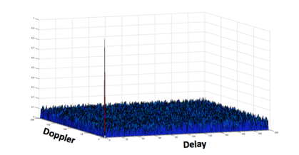
Figure 1: Profile of $\mathcal{A}(\varphi,\varphi)$ for $\varphi$ pseudo-random sequence.

I-C Ambiguity Function and Pseudo-Random Method

A classical method to estimate the channel parameters in (I-B.1) is the pseudo-random method [2, 3, 4, 6, 7]. It uses two ingredients - the ambiguity function, and a pseudo-random sequence.

I-C1 Ambiguity Function

In order to reduce the noise component in (I-B.1), it is common to use the ambiguity function that we are going to describe now. We consider the Heisenberg operators $\pi(\tau,\omega),$ $\tau,\omega\in\mathbb{Z}_{N},$ which act on $f\in\mathcal{H}$ by

$$\left[\pi(\tau,\omega)f\right][n]=e(-2^{-1}\tau\omega)\cdot e(\omega n)\cdot f[n-\tau],$$ (I-C.1)

where $2^{-1}$ denotes $(N+1)/2,$ the inverse of $2$ $\mathop{\mathrm{m}od}$ $N.$ Finally, the ambiguity function of two sequences $f,g\in\mathcal{H}$ is defined as the $N\times N$ matrix

$$\mathcal{A(}f,g)[\tau,\omega]=\left\langle\pi(\tau,\omega)f,g\right\rangle,\text{ \ }\tau,\omega\in\mathbb{Z}_{N},$$ (I-C.2)

where $\langle\mbox{ },\mbox{ }\rangle$ denotes the standard inner product on $\mathcal{H}$.

Remark I-C.1 (Fast Computation of Ambiguity Function)

The restriction of the ambiguity function to a line in the delay-Doppler plane, can be computed in $O(N\log N)$ arithmetic operations using fast Fourier transform [5]. For more details, including explicit formulas, see Section V of [1]. Overall, we can compute the entire ambiguity function in $O(N^{2}\log N)$ operations.

For $R$ and $S$ satisfying (I-B.1), the law of the iterated logarithm implies that, with probability going to one, as $N$ goes to infinity, we have

$$\mathcal{A}(S,R)[\tau,\omega]=\mathcal{A}(S,H(S))[\tau,\omega]+\varepsilon_{N},$$ (I-C.3)

where $\left|\varepsilon_{N}\right|\leq\sqrt{2\log\log N}/\sqrt{N\cdot SNR},$ with $SNR$ denotes the signal-to-noise ratio.

Remark I-C.2 (Noise)

It follows from the equation (I-C.3), that for a reasonable noise level, it is sufficient to suggest a channel estimation method which finds channel parameters by analyzing the values of $\mathcal{A}(S,H(S))$.

I-C2 Pseudo-Random Sequences

We will say that a norm-one sequence $\varphi\in\mathcal{H}$ is $B$-pseudo-random, $B\in\mathbb{R}$—see Figure 1 for illustration—if for every $\left(\tau,\omega\right)\neq(0,0)$ we have

$$\left|\mathcal{A}(\varphi,\varphi)[\tau,\omega]\right|\leq B/\sqrt{N}.$$ (I-C.4)

There are several constructions of families of pseudo-random (PR) sequences in the literature (see [2, 3] and references therein).

I-C3 Pseudo-Random Method

Consider a pseudo-random sequence $\varphi$, and assume for simplicity that $B=1$ in (I-C.4). Then we have

$$\mathcal{A}(\varphi,H(\varphi))[\tau,\omega]$$ (I-C.5)

$$= \left\{\begin{array}[]{c}\widetilde{\alpha}_{k}+\mathop{\textstyle\sum}\limits_{j\neq k}\widetilde{\alpha}_{j}/\sqrt{N},\text{ \ if }\left(\tau,\omega\right)=\left(\tau_{k},\omega_{k}\right),\text{ }1\leq k\leq r;\\ \mathop{\textstyle\sum}\limits_{j}\widehat{\alpha}_{j}/\sqrt{N},\text{ \ \ \ \ \ otherwise, \ \ \ \ \ \ \ \ \ \ \ \ \ \ \ \ \ \ \ \ \ \ \ \ \ \ }\end{array}\right.$$ (I-C.8)

where $\widetilde{\alpha}_{j},$ $\widehat{\alpha}_{j},$ $1\leq j\leq r,$ are certain multiples of the $\alpha_{j}$’s by complex numbers of absolute value less or equal to one. In particular, we can compute the delay-Doppler parameter $\left(\tau_{k},\omega_{k}\right)$ if the associated attenuation coefficient $\alpha_{k}$ is sufficiently large. It appears as a peak of $\mathcal{A}(\varphi,H(\varphi)).$ Finding the peaks of $\mathcal{A}(\varphi,H(\varphi))$ constitutes the pseudo-random method. Notice that the arithmetic complexity of the pseudo-random method is $O(N^{2}\log N),$ using Remark I-C.1. For applications to sensing, that require sufficiently high frequency resolution, we will need to use sequences of large length $N$. Hence, the following is a natural problem.

Problem I-C.3 (Arithmetic Complexity)

Solve Problem I-B.2, with method for extracting the channel parameters which requires almost linear arithmetic complexity.

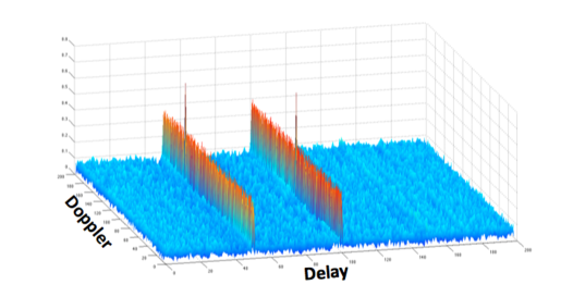
Figure 2: Profile of $\mathcal{A(}f_{L},H(f_{L}))$ for flag $f_{L},$ $L=\{(0,\omega)\},$ $N=199,$ and channel parameters $(50,150)$, $(100,100),$ with attenuation coefficients $0.7,$ $0.7,$ respectively.

I-D Flag Method

In [1] the flag method was introduced in order to deal with the complexity problem. It computes the $r$ channel parameters in $O(rN\log N)$ arithmetic operations. For a given line $L$ in the plane $\mathbb{Z}_{N}\times\mathbb{Z}_{N},$ one construct a sequence $f_{L}$—called flag—with ambiguity function $\mathcal{A(}f_{L},H(f_{L}))$ having special profile—see Figure 2 for illustration. It is essentially supported on shifted lines parallel to $L$, that pass through the delay-Doppler shifts of $H$, and have peaks there. This suggests a simple algorithm to extract the channel parameters. First compute $\mathcal{A(}f_{L},H(f_{L}))$ on a line $M$ transversal to $L,$ and find the shifted lines on which $\mathcal{A(}f_{L},H(f_{L}))$ is supported. Then compute $\mathcal{A(}f_{L},H(f_{L}))$ on each of the shifted lines and find the peaks. The overall complexity of the flag algorithm is therefore $O(rN\log N)$, using Remark I-C.1. If $r$ is large, it might be computationally insufficient.

I-E Incidence and Cross Methods

In these notes we suggest two new schemes for channel estimation that have much better arithmetic complexity than previously known methods. The schemes are based on the use of double and triple chirp sequences.

I-E1 Incidence Method

We propose to use triple-chirp sequences for channel estimation. We associate with three distinct lines $L,M$, and $M^{\circ}$ in $\mathbb{Z}_{N}\times\mathbb{Z}_{N}$, passing through the origin, a sequence $C_{L,M,M^{\circ}}\in\mathcal{H}$. This sequence has ambiguity function essentially supported on the union of $L$, $M$, and $M^{\circ}$. As a consequence—see Figure 3 for illustration—the ambiguity function $\mathcal{A}(C_{L,M,M^{\circ}},H(C_{L,M,M^{\circ}}))$ is essentially supported on the shifted lines $\{(\tau_{k},\omega_{k})+(L\cup M\cup M^{\circ})\,|\,k=1,\ldots,r\}$. This observation, which constitutes the bulk of the incidence method, enables a computation in $O(N\log{N}+r^{3})$ arithmetic operations of all the time-frequency shifts (see Section III). In addition, the estimation of the corresponding $r$ attenuation coefficients takes $O(r)$ operations. Hence, the overall complexity of incidence method is $O(N\log{N}+r^{3})$ operations.

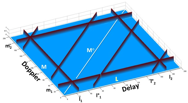
Figure 3: Essential support of the ambiguity function $\mathcal{A}(C_{L,M,M^{\circ}},H(C_{L,M,M^{\circ}}))$, where $L$ is the delay line, $M$ is the Doppler line, and $M^{\circ}$ is a diagonal line, and the support of $H$ consists two parameters. Points of $\mathbb{Z}_{N}\times\mathbb{Z}_{N}$ through them pass three lines are the true delay-Doppler parameters of $H$.

I-E2 Cross Method

We propose to use double-chirp sequences for channel estimation. For two distinct lines $L$ and $M$ in $\mathbb{Z}_{N}\times\mathbb{Z}_{N}$, passing through the origin, we introduce a sequence $C_{L,M}\in\mathcal{H}$ with ambiguity function supported on $L$, and $M$. Under genericity assumptions—see Figure 4 for illustration—the essential support of $\mathcal{A}(C_{L,M},H(C_{L,M}))$ lies on $r\times r$ grid generated by shifts of the lines $L$, and $M$. Denote by $v_{ij}=l_{i}+m_{j},\mbox{ }l_{i}\in L,m_{j}\in M;\mbox{ }1\leq i,j\leq r,$ the intersection points of the lines in the grid. Using Remark I-C.1 we find all the points $v_{ij},1\leq i,j\leq r,$ in $O(N\log{N})$ operations. The following matching problem arises: Find the $r$ points from $v_{ij}$, $1\leq i,j\leq r,$ which belong to the support of $H$. To suggest a solution, we use the values of the ambiguity function to define a certain simple hypothesis function $h:L\times M\to\mathbb{C}$ (see Section IV). We obtain:

Theorem I-E.1 (Matching)

Suppose $v_{ij}=l_{i}+m_{j}$ is a delay-Doppler shift of $H,$ then $h(l_{i},m_{j})=0.$

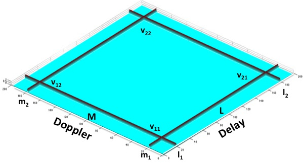
Figure 4: Essential support of the ambiguity function $\mathcal{A}(C_{L,M},H(C_{L,M}))$, where $L$ is the delay line, $M$ is the Doppler line, and the support of $H$ consists two parameters.

The cross method makes use of Theorem I-E.1 and checks the values $h(l_{i},m_{j}),\mbox{ }1\leq i,j\leq r$. If a value is less than a priori chosen threshold, then the algorithm returns $v_{ij}=l_{i}+m_{j}$ as one of the delay-Doppler parameters. To estimate the attenuation coefficient corresponding to $v_{ij}$ takes $O(1)$ arithmetic operations (see details in Section IV). Overall, the cross method enables channel estimation in $O(N\log{N}+r^{2})$ arithmetic operations.

II Chirp, Double-Chirp, and Triple-Chirp Sequences

In this section we introduce the chirp, double-chirp, and triple-chirp sequences, and discuss their correlation properties.

II-A Definition of the Chirp Sequences

We have $N+1$ lines in the discrete delay-Doppler plane $V=\mathbb{Z}_{N}\times\mathbb{Z}_{N}.$ For each $a\in\mathbb{Z}_{N}$ we have the line $L_{a}=\left\{(\tau,a\tau);\tau\in\mathbb{Z}_{N}\right\}$ of finite slope $a,$ and in addition we have the line of infinite slope $L_{\infty}=\left\{(0,\omega);\text{ }\omega\in\mathbb{Z}_{N}\right\}.$ We have the orthonormal basis for $\mathcal{H}$

$$\mathcal{B}_{L_{a}}=\left\{C_{L_{a,b}}\text{; }b\text{ }\in\mathbb{Z}_{N}\right\},$$

of chirp sequences associated with $L_{a}$, where

$$C_{L_{a,b}}[n]=e(2^{-1}an^{2}-bn)/\sqrt{N},n\in\mathbb{Z}_{N}.$$

In addition, we have the orthonormal basis

$$\mathcal{B}_{L_{\infty}}=\left\{C_{L_{{}_{\infty},b}}\text{ ; }b\text{ }\in\mathbb{Z}_{N}\right\},$$

of chirp sequences associated with $L_{\infty}$, where

$$C_{L_{{}_{\infty},b}}=\delta_{b},$$

denotes the Dirac delta sequence supported at $b.$

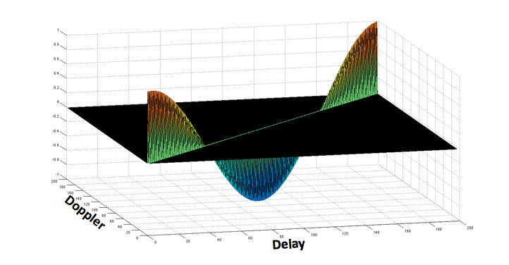
Figure 5: Plot (real part) of $\mathcal{A}(C_{L_{1,1}},C_{L_{1,1}}),$ for chirp $C_{L_{1,1}}[n]=e[2^{-1}n^{2}-n]$, associated with the line $L_{1}=\{(\tau,\tau)\}.$

II-B Chirps as Eigenfunctions of Heisenberg Operators

The Heisenberg operators (I-C.1) satisfy the commutation relations

$$\pi(\tau,\omega)\pi(\tau^{\prime},\omega^{\prime})=e(\omega\tau^{\prime}-\tau\omega^{\prime})\cdot\pi(\tau^{\prime},\omega^{\prime})\pi(\tau,\omega),$$ (II-B.1)

for every $(\tau,\omega),(\tau^{\prime},\omega^{\prime})\in V.$ In particular, for a given line $L\subset V,$ we have the family of commuting operators $\pi(l),$ $l\in L.$ Hence they admit an orthonormal basis $\mathcal{B}_{L}$ for $\mathcal{H}$ of common eigenfunctions. Important property of the chirp sequences is that for every chirp sequence $C_{L}\in\mathcal{B}_{L}$, there exists a character $\psi_{L}:L\to\mathbb{C}^{*}$, i.e. $\psi_{L}(l+l^{\prime})=\psi_{L}(l)\psi_{L}(l^{\prime}),$ $l,l^{\prime}\in L$, such that

$$\pi_{L}(l)C_{L}=\psi_{L}(l)C_{L},\mbox{ for every }l\in L.$$

This implies—see Figure 5—that for every $C_{L}\in\mathcal{B}_{L}$ we have

$$\mathcal{A}(C_{L},C_{L})[v]=\left\{\begin{array}[]{c}\psi_{L}(v)\text{ \ if }v\in L;\\ \ \ 0\text{ \ \ \ \ \ \ \ if }v\notin L.\text{ \ }\end{array}\right.$$ (II-B.2)

It is not hard to see [4] that for distinct lines $L$, and $M$, and two chirps $C_{L}\in\mathcal{B}_{L},C_{M}\in\mathcal{B}_{M}$ we have

$$\left|\mathcal{A(}C_{L},C_{M})[v]\right|=1/\sqrt{N},\ \ \ \ \mbox{ for every }v\in V.$$ (II-B.3)

II-C Double-Chirp Sequences

For any two distinct lines $L,M\in V$, and two characters $\psi_{L},\psi_{M}$ on them, respectively, denote by $C_{L}$ the chirp corresponding to $L$ and $\psi_{L}$, and by $C_{M}$ the chirp corresponding to $M$, and $\psi_{M}$. We define the double-chirp sequence

$$C_{L,M}=(C_{L}+C_{M})/\sqrt{2}.$$

It follows from (II-B.2) and (II-B.3) that for the line $K=L$, or $M$, we have

$$\mathcal{A}(C_{K},C_{L,M})[v]\approx\left\{\begin{array}[]{c}\psi_{K}(v)/\sqrt{2}\text{ \ \ \ if }v\in K;\\ \ \ 0\text{ \ \ \ \ \ \ \ \ \ \ \ \ \ \ \ if }v\notin K.\text{ \ }\end{array}\right.$$

II-D Triple-Chirp Sequences

Consider three distinct lines $L,M,M^{\circ}\in V$, and three characters $\psi_{L},\psi_{M},$ $\psi_{M^{\circ}}$ on them, respectively. Denote by $C_{L},C_{M}$ and $C_{M^{\circ}}$ the chirps corresponding to $L,M$ and $M^{\circ}$, and $\psi_{L},\psi_{M},$ and $\psi_{M^{\circ}}$, respectively. We define the triple-chirp sequence

$$C_{L,M,M^{\circ}}=(C_{L}+C_{M}+C_{M^{\circ}})/\sqrt{3}.$$

It follows from (II-B.2) and (II-B.3) that for the line $K=L,M$ or $M^{\circ}$, we have

$$\mathcal{A}(C_{K},C_{L,M,M^{\circ}})[v]\approx\left\{\begin{array}[]{c}\psi_{K}(v)/\sqrt{3}\text{ \ \ \ \ if }v\in K;\\ \ \ 0\text{ \ \ \ \ \ \ \ \ \ \ \ \ \ \ \ \ if }v\notin K.\text{ \ }\end{array}\right.$$

III Incidence Method

We describe—see Figure 3 for illustration—the incidence algorithm.

Incidence Algorithm

Input:

 Randomly chosen lines $L$, $M$, and $M^{\circ}$, and characters $\psi_{L},\psi_{M},\psi_{M^{\circ}}$ on them, respectively. Echo $R_{L,M,M^{\circ}}$ of the triple-chirp $C_{L,M,M^{\circ}}$, threshold $T>0$, and value of $SNR$.

Output:

    Channel parameters.

1. Compute $\mathcal{A(}C_{M},R_{L,M,M^{\circ}}\mathcal{)}$ on $L$, obtain peaks at $l_{1},...,l_{r_{1}}.\vskip 3.0pt plus 1.0pt minus 1.0pt$

2. Compute $\mathcal{A(}C_{L},R_{L,M,M^{\circ}}\mathcal{)}$ on $M,$ obtain peaks at $m_{1},...,m_{r_{2}}.\vskip 3.0pt plus 1.0pt minus 1.0pt$

3. Compute $\mathcal{A(}C_{M^{\circ}},R_{L,M,M^{\circ}}\mathcal{)}$ on $L,$ obtain peaks at $l_{1}^{\circ},...,l_{r_{3}}^{\circ}.\vskip 3.0pt plus 1.0pt minus 1.0pt$

4. Find $v_{ij}=l_{i}+m_{j}$ which solve $l_{i}+m_{j}\in M^{\circ}+l_{k}^{\circ},$ $1\leq i\leq r_{1}$, $1\leq j\leq r_{2}$, $1\leq k\leq r_{3}$.

5. For every delay-Doppler parameter $v_{ij}=l_{i}+m_{j}$ found in the previous step, compute $\alpha_{v_{ij}}=\sqrt{3}\mathcal{A(}C_{L},R_{L,M,M^{\circ}}\mathcal{)}[m_{j}]\psi_{L}(l_{i})$. Return the parameter $(\alpha_{v_{ij}},v_{ij})$.

IV Cross Method

Let $C_{L,M}$ be the double-chirp sequence associated with the lines $L,M\subset V$, and the characters $\psi_{L}$, and $\psi_{M}$, on $L$, and $M$, correspondingly. We define hypothesis function $h:L\times M\rightarrow\mathbb{C}$ by

$$h(l,m) = \mathcal{A}(C_{L},R_{L,M})[m]\cdot\psi_{L}[l]$$

$$-\mathcal{A}(C_{M},R_{L,M})[l]\cdot e(\Omega[l,m])\cdot\psi_{M}[m],$$

where $\Omega:V\times V\rightarrow\mathbb{Z}_{N}$ is given by $\Omega[(\tau,\omega),(\tau^{\prime},\omega^{\prime})]=\tau\omega^{\prime}-\omega\tau^{\prime}.\vskip 3.0pt plus 1.0pt minus 1.0pt$ Below we describe—see Figure 4—the Cross Algorithm.

Cross Algorithm

Input:

  Randomly chosen lines $L$, $M$, and characters $\psi_{L},\psi_{M}$ on them, respectively. Echo $R_{L,M}$ of the double-chirp $C_{L,M}$; thresholds $T_{1},T_{2}>0$, and the value of $SNR$.

Output:

    Channel parameters.

1. Compute $\mathcal{A}(C_{M},R_{L,M})$ on $L,$ and take the $r_{1}$ peaks located at points $l_{i},$ $1\leq i\leq r_{1}\vskip 3.0pt plus 1.0pt minus 1.0pt$.

2. Compute $\mathcal{A}(C_{L},R_{L,M})$ on $M,$ and take the $r_{2}$ peaks located at the points $m_{j},1\leq j\leq r_{2}\vskip 3.0pt plus 1.0pt minus 1.0pt$.

3. Find $v_{ij}=l_{i}+m_{j}$ which solve $|h(l_{i},m_{j})|\leq T_{2}\sqrt{2\log\log(N)}/\sqrt{N\cdot SNR}$, where $1\leq i\leq r_{1}$, $1\leq j\leq r_{2}$.

4. For every delay-Doppler parameter $v_{ij}=l_{i}+m_{j}$ found in the previous step, compute $\alpha_{v_{ij}}=\sqrt{2}\mathcal{A(}C_{L},R_{L,M}\mathcal{)}[m_{j}]\psi_{L}(l_{i})$. Return the parameter $(\alpha_{v_{ij}},v_{ij})$.

V Conclusions

In these notes we present the incidence and cross methods for efficient channel estimation. These methods, in particular, suggest solutions to the arithmetic complexity problem. Low arithmetic complexity enables working with sequences of larger length $N$, and hence higher velocity resolution of channel parameters. We summarize these important features in Figure 6, and putting them in comparison with the pseudo-random (PR) and Flag methods.

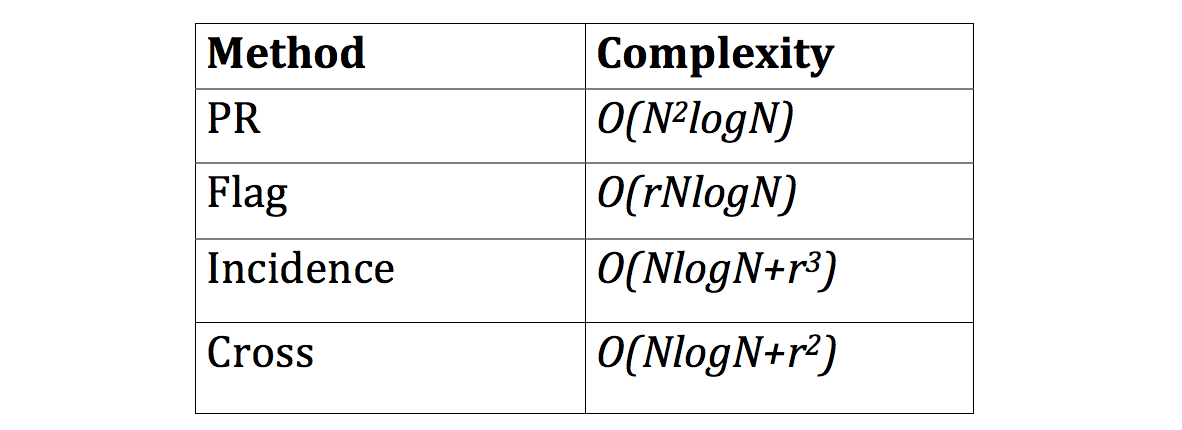
Figure 6: Comparing methods, with respect to arithmetic complexity for $r$ channel parameters, and sensibility of the parameters in terms of magnitude of attenuation coefficients (noiseless scenario).

Remark V-.1

Both new methods are robust to a certain degree of noise since they use the values of the ambiguity functions, which is a sort of averaging.

Acknowledgements. We are grateful to our collaborators A. Sayeed, and O. Schwartz, for many discussions related to the research reported in these notes.

References

- [1] Fish A., Gurevich S., Hadani R., Sayeed A., and Schwartz O., Delay-Doppler Channel Estimation with Almost Linear Complexity. Accepted for publication in IEEE Transaction on Information Theory (2013).
- [2] Golomb, S.W., and Gong G., Signal design for good correlation. For wireless communication, cryptography, and radar. Cambridge University Press, Cambridge (2005).
- [3] Gurevich S., Hadani R., and Sochen N., The finite harmonic oscillator and its applications to sequences, communication and radar . IEEE Transactions on Information Theory, vol. 54, no. 9, September 2008.
- [4] Howard S. D., Calderbank, R., and Moran W., The finite Heisenberg–Weyl groups in radar and communications. EURASIP J. Appl. Signal Process (2006).
- [5] Rader C. M., Discrete Fourier transforms when the number of data samples is prime. Proc. IEEE 56, 1107–1108 (1968).
- [6] Tse D., and Viswanath P., Fundamentals of Wireless Communication. Cambridge University Press (2005).
- [7] Verdu S., Multiuser Detection, Cambridge University Press (1998).