Carbon and Oxygen Abundances in Cool Metal-rich Exoplanet Hosts: A Case Study of the C/O Ratio of 55 Cancri*

Abstract

The super-Earth exoplanet 55 Cnc e, the smallest member of a five-planet system, has recently been observed to transit its host star. The radius estimates from transit observations, coupled with spectroscopic determinations of mass, provide constraints on its interior composition. The composition of exoplanetary interiors and atmospheres are particularly sensitive to elemental C/O ratio, which to first order can be estimated from the host stars. Results from a recent spectroscopic study analyzing the 6300 Å [O I] line and two C I lines suggest that 55 Cnc has a carbon-rich composition (C/O=1.12$\pm$0.09). However oxygen abundances derived using the 6300 Å [O I] line are highly sensitive to a Ni I blend, particularly in metal-rich stars such as 55 Cnc ([Fe/H]$=$0.34$\pm$0.18). Here, we further investigate 55 Cnc’s composition by deriving the carbon and oxygen abundances from these and additional C and O absorption features. We find that the measured C/O ratio depends on the oxygen lines used. The C/O ratio that we derive based on the 6300 Å [O I] line alone is consistent with the previous value. Yet, our investigation of additional abundance indicators results in a mean C/O ratio of 0.78$\pm$0.08. The lower C/O ratio of 55 Cnc determined here may place this system at the sensitive boundary between protoplanetary disk compositions giving rise to planets with high ($>$0.8) versus low ($<$0.8) C/O ratios. This study illustrates the caution that must applied when determining planet host star C/O ratios, particularly in cool, metal-rich stars.

1 Introduction

Exoplanet observational surveys reveal a large and diverse population of planets with masses between a few and $\sim$20 Earth masses, approaching the size of Solar System terrestrial planets (Lovis et al. 2009; Sumi et al. 2010; Borucki et al. 2011). A member of the five-planet system orbiting a nearby ($\sim$12.3 pc) G8V star every 18 hours, 55 Cnc e (e.g., McArthur et al. 2004; Winn et al. 2011) belongs to the small sample of confirmed terrestrial-sized planets that transit their host stars. Observations of 55 Cnc e have provided a well-constrained mass (8.37$\pm$0.38 M_⊕; Endl et al. 2012) and radius (e.g., 1.990${}^{+0.084}_{-0.080}$ R_⊕ in the visible; Dragomir et al. 2013), yielding the density of the super-Earth exoplanet (5.86${}^{+0.79}_{-0.76}$ g cm^-3), which can then be used to constrain its interior composition.

The observed mass and radius of 55 Cnc e place it between the high-density “super-Mercuries”, like CoRoT-7b and Kepler-10b, and the volatile-rich small planets, like Kepler-11b and GJ 1214b. It intersects the threshold mass and radius between interior compositions that necessarily require volatiles and ones that may be rocky (see, for example, Gillon et al. 2012, Figure 5). Hence a massive water envelope ($\simeq 10$%), which would be super-critical given 55 Cnc e’s irradiation, over an Earth-like interior (33% iron core above 67% silicate mantle with 10% iron by mol), has been suggested to explain the observed mass and radius (Winn et al. 2011; Demory et al. 2011; Gillon et al. 2012).

Recently Madhusudhan et al. (2012) suggest an alternative and carbon-rich composition of 55 Cnc e, garnering the super-Earth popular attention as “the diamond planet.” Measurements of the carbon and oxygen abundances from two C I lines (5052 Å, 5135 Å) and one forbidden [O I] line (6300 Å) indicate a C/O ratio of 1.12$\pm$0.19 (Delgado Mena et al. 2010), i.e., a highly carbon-rich star compared to the solar C/O$\sim$0.50 (Asplund et al. 2005). If the disk shared the host star’s composition, and the host star is carbon-rich, then the planetesimals accreted during the formation of 55 Cnc e were likely Fe- and C-rich (Bond et al. 2010; Madhusudhan et al. 2012). To investigate the composition of the possibly carbon-rich exoplanet, Madhusudhan et al. (2012) consider two families of carbon-rich interior models of 55 Cnc e, consisting of layers, from inner to outer, of Fe-SiC-C and Fe-MgSiO₃-C. Included in their carbon equation of state (EOS) are the graphite EOS at low pressures, the phase transition to diamond between 10 GPa$<$P$<$1000 GPa, and the Thomas-Fermi-Dirac EOS at high pressures. Madhusudhan et al. (2012) find a wide range of compositions are possible, including extreme combinations like (Fe, SiC, C) = (33%, 0%, 67%), and the best match to 55 Cnc e’s observations depends on the adopted radius measurement, and the conditions in the protoplanetary disk, e.g. temperature, at which the building blocks of the planet condense.

The exact composition of 55 Cnc e depends on the primary source of accreted planetesimals, the ratio of gas to solid material accreted, and how isolated the atmosphere was from the interior (e.g., Öberg et al. 2011; Bond et al. 2010). While the C/O ratios of protoplanetary disks likely change with time and distance (Öberg et al. 2011), the assumption that the disk bears roughly the same composition of the host star is a reasonable first-order one for estimating refractory condensates forming rocky planets (Bond et al. 2010; Carter-Bond et al. 2012; Johnson et al. 2012). Thus constraining the elemental abundances of the host star is a crucial step in determining the composition of 55 Cnc e.

Yet determinations of the stellar C/O ratios can be challenging. The 6300 Å forbidden oxygen line is chosen in many studies, including the previous study of 55 Cnc, because of it has been shown to give reliable abundances in LTE analyses (e.g., Schuler et al. 2011; Cuhna et al. 1998). However, this line is weak and blended with a Ni I line, the treatment of which significantly affects the derived oxygen abundance, particularly at high metallicities. Here we further investigate the C/O ratio of 55 Cnc by determining the nickel abundance from the data and reanalyzing the original line used to study its oxygen content, as well as the same two C I lines. We also determine the oxygen abundance from an additional forbidden [O I] line at 6363 Å and the O I triplet at 7774 Å, and the carbon abundance from two molecular C₂ features. This work aims to determine whether the stellar abundance indicates a diamond-rich composition of 55 Cnc, and to explore the difficulties in deriving the C/O ratios in cool high-metallicity stars.

2 Observations and Abundance Analysis

2.1 Data

We analyze Keck/HIRES (Vogt et al. 1994) archive spectra of 55 Cnc (PID H32bH; PI Shkolnik) taken across four nights in January 2006, covering the wavelength range 3360-8100 Å with the kv370 filter. Individual frame exposure times range from 20 to 120 sec and S/N ratios range from $\sim$170 to 350 around the 6300 Å [O I] line; the 35 spectra combined yield a S/N of $\sim$1270 around the 6300 Å [O I] line. To enable differential abundance determinations relative to the Sun, we also analyze three solar spectra of reflected light from Vesta (PID N014Hr; PI Marcy). These data were taken in April 2006 with the same filter, and with individual frame exposure times $\sim$230 sec; combined the spectra yield a S/N ratio $\sim$315 around the 6300 Å [O I] line. All archive HIRES data were reduced with the MAKEE pipeline using corresponding bias ($\sim$3), flat ($\sim$30), ThAr (arc), and trace star frames for each target frame separately. The frames were then combined in IRAF.

2.2 Stellar Parameters

The stellar parameters ($T_{\rm{eff}}$, log $g$, microturbulence [$\xi$]) and metallicity ([Fe/H]) for 55 Cnc were derived following the procedures in Schuler et al. (2011) and Teske et al. (2013). We measured equivalent widths (EWs) of 55 Fe I lines and 9 Fe II lines in 55 Cnc and the Sun (with the one-dimensional spectrum analysis package SPECTRE; Fitzpatrick & Sneden 1987). We fit Gaussian profiles to each absorption line (some weaker lines were fit with a Simpson’s Rule integration).

The abundances were determined using an updated version of the LTE spectral analysis code MOOG (Sneden 1973), with model atmospheres interpolated from the Kurucz ATLAS9 grids. To fulfill the requirement of excitation equilibrium, the [Fe/H] values derived from the Fe I lines must not show any correlation with the lower level excitation potential ($\chi$); this was used to determine $T_{\rm{eff}}$. In addition, the $\xi$ was determined by requiring [Fe/H] values derived from the Fe I lines to show no correlation with the measured EW values (specifically the reduced equivalent width, log(EW/$\lambda$)). Also, the averaged [Fe/H] values derived from the Fe I and Fe II lines must be equal – the requirement of ionization equilibrium; this sets the surface gravity (log $g$).

Initial values of $T_{\rm{eff}}$, log $g$, microturbulence ($\xi$), and [Fe/H] of 55 Cnc from the literature were taken as starting values in the iterative process of determining 55 Cnc’s stellar parameters. Prior to this iterative scheme, we ensured that there was no correlation between $\chi$ and the reduced EWs of the Fe I lines analyzed; unique solutions for $T_{\rm{eff}}$ and $\xi$ are only possible if there is no such correlation. The measured reduced EWs were used to determine abundances (using the“abfind” task in MOOG), and the stellar parameters were altered and new [Fe/H] abundances determined until the criteria above were met. The log$N$(Fe) values from each line were normalized to solar values on a line-by-line basis. The log$N$(Fe) value for the Sun was determined with our solar spectrum and a solar Kurucz model with $T_{\rm{eff}}$=5777, log $g$=4.44, [Fe/H]=0.00, and $\xi$=1.38.

2.2.1 Uncertainties in $T_{\rm{eff}}$, log $g$, and $\xi$

The errors in $T_{\rm{eff}}$ and $\xi$ were calculated by forcing 1$\sigma$ correlations in the relations between [Fe I/H] and $\chi$, and between [Fe I/H] and reduced EW, respectively. The change in $T_{\rm{eff}}$ or $\xi$ required to cause a correlation coefficient $r$ significant at the 1$\sigma$ level was adopted as the uncertainty in these parameters. The uncertainty in log $g$ was calculated differently, through an iterative process described in detail in Baubar & King (2010). The difference between the Fe I and Fe II abundances is dependent on the log $g$ value, so the uncertainty in log $g$ is tied to the uncertainties in both [Fe I/H] and [Fe II/H]. To calculate the uncertainty in log $g$, its value is perturbed until the difference between [Fe I/H] and [Fe II/H] is equal to the combined uncertainty in [Fe I/H] and [Fe II/H]. Uncertainties in [Fe I/H] and [Fe II/H] are calculated from the quadratic sum of the individual uncertainties in these abundances due to the derived uncertainties in $T_{\rm{eff}}$ and $\xi$ as well as the uncertainty in the mean ($\sigma_{\mu}$) of each abundance (see §2.3.3). The same procedure is then repeated, including the first iteration’s log $g$ uncertainty (the $\delta$log $g$) in the calculation of the Fe abundance uncertainties. The final log $g$ uncertainty is then the difference between the log $g$ value originally derived and that obtained from this second iteration of the error calculation.

Table 1 lists the final derived stellar parameters and 1$\sigma$ uncertainties, as well as several literature values for comparison. The errors derived here are larger than those from previous studies, in which 55 Cnc was part of a large ensemble of stars analyzed. We note, however, that using the same stellar parameter analysis and error calculation method on stars with temperatures closer to the Sun than 55 Cnc, we obtain errors on $T_{\rm{eff}}$, log $g$, and $\xi$ that are more similar to typical error values quoted in the literature. Larger errors for cooler stars are also found by Teske et al. (2013), Ammler-von Eiff et al. (2009), and Torres et al. (2012), studies that determine stellar parameters and errors with methods similar to those used in this work. Our conservative stellar parameter errors for 55 Cnc also propagate through the abundance errors, as discussed in §2.3.3.

2.3 Stellar Abundances

Abundances of iron and nickel ([Fe/H], [Ni/H]) were normalized to solar values on a line-by-line basis, derived directly from EW measurements of spectral lines in 55 Cnc and the Sun with the “abfind” driver in MOOG. Lines lists for Fe and Ni are from Schuler et al. (2011), and lower level excitation potentials ($\chi$) and transition probabilities (log $gf$) are taken from the Vienna Atomic Line Database (VALD; Kupka et al. 1999), although we note that the log $gf$ values do not have a impact on the final abundances due to our strictly differential analysis. The EW measurements (and results of our synthesis analysis, described below) are shown in Table 2, along with the wavelength, $\chi$, log $gf$, EWs, and line-by-line abundances for each element for the Sun and 55 Cnc.

2.3.1 Carbon Abundance

The carbon abundance for 55 Cnc was derived from two C I lines at 5052 Å and 5380 Å and two C₂ molecular features at 5086.3 Å and 5135.6 Å. The two C I lines have been shown to provide reliable abundances in solar-type stars, with negligible NLTE corrections ($\leq$0.05 dex; Asplund et al. 2005; Takeda & Honda 2005; Caffau et al. 2010). We derived [C/H] from these lines with our EW measurements, with atomic parameters from Hibbert et al. (1993) (see Table 2). The log$N$(C)_⊙ values we derive with our EW measurements are a good match, with $\leq$0.02 dex difference, to the log$N$(C)_⊙ values derived by Caffau et al. (2010) from these lines using 3D hydrodynamical simulations of the Sun.

The C₂ lines are blends of multiple components of the Swan system, requiring spectral synthesis (matching a set of trial synthetic spectra to the observed spectrum) for abundance derivation. We used the line lists of Schuler et al. (2011) and C₂ molecular data from Lambert & Ries (1981), modified in that paper from theoretical values to fit the Kurucz solar flux atlas assuming a solar abundance of log$N$(C)_⊙=8.39 (Asplund et al. 2005). A dissociation energy of 6.297 eV was assumed for C₂ (Urdahl et al. 1991). The synthesized spectra were convolved with a Gaussian profile, based on near-by unblended lines, to represent the instrument PSF, stellar macroturbulence, and rotational broadening; the remaining free parameters were continuum normalization, line broadening, wavelength shift, and carbon abundance. The best fits to the synthesized spectra for the C₂ lines were determined by minimizing the deviations between the observed and synthetic spectra.

As evidenced in Table 3, the [C/H] abundance derived from the C I is slightly lower than that derived from the C₂ lines; this as also observed by Asplund et al. (2005) in both 3D hydrodynamical and 1D models of the solar atmosphere. However, our [C/H]${}_{\rm{C\,I}}$ value overlaps with the [C/H]${}_{\rm{C_{2}}}$ value within errors.

2.3.2 Oxygen Abundance

Oxygen abundances were derived from three separate indicators and are listed in Table 3. The forbidden [O I] line at 6300.3 Å is well-described by LTE (e.g. Takeda 2003). This line is blended with a Ni I line (2 isotopic components) with a strength $\sim$55% of the [O I] line in the Sun (Caffau et al. 2008), requiring spectral synthesis similar to the C₂ lines. Due to [Ni/Fe] increasing with [Fe/H] (Bensby et al. 2003), the Ni I blend becomes more important at higher metallicities, the regime in which most high-C/O values for exoplanet host stars have been found (Nissen 2013). When determining the oxygen abundance, we used the nickel abundance measured directly from our 55 Cnc spectrum, log$N$(Ni) = 6.68 derived from 14 lines, with log $gf$(⁶⁰Ni)=-2.965 and log $gf$(⁵⁸Ni)=-2.275 (Bensby et al. 2004). For the 6300.3 Å line we adopted the Storey & Zeippen (2000) log $gf=$-9.717 value, based on their forbidden transition probability calculations including both relativistically-corrected magnetic dipole and electric quadruopole contributions.

The [O I] 6363.79 Å forbidden line (log $gf=-$10.185, Storey & Zeippen 2000) is weaker than the 6300 Å line, and is also blended with CN lines (6363.776 Å and 6363.846 Å; Asplund et al. 2004). We again determined [O/H] from this line using spectral synthesis, with a line list compiled mostly from Kurucz and supplemented with lines from Asplund et al. (2004). For this analysis, we used the carbon abundance derived here, and a solar-scaled nitrogen abundance.

The O I triplet lines at 7771-7775 Å are unblended and prominent, hence we analyzed them with direct EW measurements (see Table 2). Here we did not include the 7774 Å component because the line appears slightly asymmetric, and gives an anomalously high ($+$0.10 dex) abundance compared to the other two components, 7771.94 Å ($\chi$=9.15 eV, log $gf$=0.369; Hibbert et al. 1991) and 7775.4 Å ($\chi$=9.15 eV, log $gf$= 0.001; Hibbert et al. 1991). This effect is also seen in the coolest stars in Schuler et al. (2006) and Bubar & King (2010); these authors suggest it may be due to a Fe I blend at 7774.00 Å in cool metal-rich stars, but this explanation has yet to be verified.

The triplet lines are strong and form in the higher photospheric layers, and thus suffer from non-LTE (NLTE) effects due to the dilution of each line’s source function compared to the Planck function in the line-forming region (Kiselman 2001). The large energy gap between the two lowest energy levels and levels of higher energy prohibits collisional excitation from maintaining LTE, and the upper level of the triplet is underpopulated compared to the lower level (Kiselman 1993). This causes the source function to be smaller than the Planck function, leading to stronger absorption lines (Kiselman 1993; Gratton et al. 1999). Abundances derived from these lines assuming LTE are thus overestimated. The effect increases as the number of electrons in the initial (lower) transition state increases, which can be caused by decreasing gas pressures or increasing temperatures in the line-forming region, and/or an increase in the number of oxygen atoms. Thus the discrepancy between LTE and NLTE calculations and observations is more prominent for hot ($T_{\rm{eff}}\gtrsim 6000$ K) solar-metallicity dwarfs and evolved metal-poor subgiants with decreased surface gravity.

Multiple groups have prescriptions for NLTE corrections, which involve establishing the departure from LTE coefficients ($n_{\rm{NLTE}}$/$n_{\rm{LTE}}$, the ratios of the populations in NLTE and LTE) from statistical equilibrium calculations for varying stellar parameters. Takeda (2003) constructs a neutral atomic oxygen model with 87 levels and 277 radiative transitions, with atomic data from Kurucz & Bell (1995). In their atomic model, the neutral hydrogen population is taken from Kurucz LTE model atmospheres, and the photoionizing radiation is computed from the same LTE stellar atmospheres, incorporating the line opacity using Kurucz’s (1993) opacity distribution function. The effect of H I collisions is treated according to Steenbock & Holweger’s (1984) classicial formula, which is derived from Drawin’s (1968) application of Thomson’s theory for electron-atom encounters to collisions between identical particles. Takeda (2003) finds that for a given $T_{\rm{eff}}$, log $g$, and $\xi$, the NLTE correction to the oxygen abundances is a nearly monotonic function of EW. They fit the coefficients $a$ and $b$ in their relation $\Delta=a10^{bW_{\lambda}}$ based on their computed $\Delta$ values. Here we use this relation and the $a$ and $b$ coefficients corresponding to the determined parameters of 55 Cnc to yield $\Delta$ corrections to our computed LTE oxygen triplet abundances.

Ramírez et al. (2007) compute NLTE corrections using an oxygen model atom with 54 levels and 242 transitions, with atmoic data from Allende Prieto et al. (2003) and fixed temperature and electron density structures from the Kurucz LTE models. They allow the H and O level populations to depart from LTE by solving rate equations while recalculating the radiation field with the NLTE stellar atmosphere code TLUSTY (Hubey & Lanz 1995), and do not include H I collisions. Ramírez et al. (2007) construct a grid of NLTE abundances directly from curves of growth corresponding to a range of stellar parameters ($T_{\rm{eff}}$, log $g$, [Fe/H]) and provide an IDL routine to interpolate within the grid, which we used here.

Fabbian et al. (2009) construct a model atom containing 54 energy levels and 258 radiation transitions, with atomic parameters from the NIST Atomic Spectra Database and radiative and Stark parameters from VALD. They include fine-splitting of energy levels where appropriate (ground state and upper level of O I triplet), and the H I collision approximation of Steenbock & Holweger (1984) scaled by an empirical factor $S_{H}$, either =0 or =1. Fabbian et al. (2009) also include the most recent electron collision cross sections of Barklem (2007) based on quantum mechanical calculations; this gives larger NLTE corrections due to increased intersystem coupling. We obtained their grid of NLTE corrections and IDL interpolation routine, but it does not cover [Fe/H]$>$0 or log$N$(O)$>$8.83, so we extrapolated to the measurements of 55 Cnc. In order to enable direct comparison, we also interpolated Fabbian et al.’s (2009) NLTE corrections to the same scaling factor as Nissen (2013), $S_{H}=$0.85, which has been shown to yield the best agreement with observations of O I triplet in the Sun (Pereira et al. 2009).

In Table 3 we show the derived LTE [O/H] abundances from the O I triplet, and also apply the NLTE corrections of Takeda (2003), Ramírez et al. (2007), and Fabbian et al. (2009) for comparison. Overall, the NLTE corrections are between 0.06 and 0.1 dex.

2.3.3 Abundance Uncertainties

There are two components to the uncertainties in derived elemental abundances – one from stellar parameter errors and one from the dispersion in the abundances derived from different absorption lines. To determine the uncertainty due to the stellar parameters, the sensitivity of the abundance to each parameter was calculated for changes of $\pm 150$ K in $T_{\rm{eff}}$, $\pm 0.25$ dex in log $g$, and $\pm 0.30$ km s^-1 in $\xi$. For the abundances determined through spectral synthesis, models with this range of stellar parameters were compared to the data and the elemental abundance adjusted to determine the best fit. The uncertainty due to each parameter is then the product of this sensitivity and the corresponding parameter uncertainty. The second uncertainty component is the uncertainty in the mean, $\sigma_{\mu}$, for the abundances derived from the averaging of multiple lines. The total uncertainty for each abundance ($\sigma_{\rm{tot}}$) is the quadratic sum of the three individual parameter uncertainties ($T_{\rm{eff}}$, log $g$, $\xi$) and $\sigma_{\mu}$.

In the case of the O I triplet, the error on [O/H]_NLTE was calculated separately for each of the NLTE corrections we applied (see Table 3). For errors on the Ramírez et al. (2007) and Fabbian et al. (2009) NLTE abundances, we calculated their sensitivity to $\pm$150 K $T_{\rm{eff}}$ and $\pm$0.25 dex log $g$. We then combined these with $\sigma_{\mu}$ for the NLTE abundances to determine the NLTE abundance errors. Takeda (2003) NLTE corrections include a dependence on $\xi$, so we calculated the sensitivity of these NLTE abundances to $\xi$ in addition to $T_{\rm{eff}}$ and log $g$, but used changes of $\pm$1 km s^-1, $\pm$500 K, $\pm$1.0 dex, respectively, due to the grid spacing of the Takeda (2003) NLTE corrections. As with the other [O/H]_NLTE errors, we also included the $\sigma_{\mu}$ for the Takeda (2003) NLTE abundances.

The final derived stellar parameters and their 1$\sigma$ uncertainties, as well as the derived [Fe/H] and [Ni/H] values and their 1$\sigma$ uncertanties, are shown in Table 1, along with several literature values for comparsion. In Table 3 we detail the [C/H] and [O/H] values derived from different abundance indicators. Table 4 shows the range in C/O ratios resulting from the different carbon and oxygen abundance indicators. These C/O ratios were calculated with the prescription log$N_{\rm{55Cnc}}$(O)$=$derived [O/H]_55Cnc+log$N_{\odot}$(O) and log$N_{\rm{55Cnc}}$(C)$=$derived [C/H]_55Cnc+log$N_{\odot}$(C), where log$N_{\odot}$(O)$=$8.66 and log$N_{\odot}$(C)$=$8.39 (Asplund et al. 2005). The errors on the C/O value are represented by the quadratic sum of the errors in [C/H] and [O/H].

3 Results & Discussion

The stellar parameters ($T_{\rm eff}$, log g, and [Fe/H]) derived here compare well with previous determinations in Table 1. The average values from the five literature sources in Table 1 are are $T_{\rm eff}$=5268$\pm$38K, log g=4.45$\pm$0.05, and [Fe/H]=+0.32$\pm$0.03. The differences between the average values in the literature and those derived here are, in the sense of ‘this study - literature’, $\Delta T_{\rm eff}$=+82K, $\Delta$log g=-0.01 dex, and $\Delta$[Fe/H]=+0.02 dex. These differences are all within the estimated uncertainties presented here and indicate that there are not large systematic differences between this study and those published previously. This result is encouraging, given the challenging nature of characterizing the relatively rare “super-metal rich” stars with their enhanced line absorption (e.g., Cayrel de Strobel et al. 1999; Taylor 2002; Gonzalez & Vanture 1998; Feltzing & Gonzalez 2001). Clearly, 55 Cnc is a well-established metal-rich star that happens to be nearby, hosts a multiple-planet system, and exhibits planetary transits.

Due to its proximity to the Sun and favorable multi-planet geometry, 55 Cnc is an important object in the study of planet formation, and thus it is useful to constrain as many of its fundamental properties as possible. The age of 55 Cnc is uncertain – the $T_{\rm eff}$ or color dependencies as a function of isochrone age, even for its known metallicity, render age estimates uncertain by several Gyr’s. Ages from $\sim$3-9 Gyr can fit the position of M_V versus $T_{\rm eff}$, or ($V$-$K$), or ($B$-$V$) isochrones (e.g., Fuhrmann, Pfeiffer & Bernkopf 1998). Other indicators tend to result in ages from 2-5 Gyr, such as Eggen’s (1985) identification of 55 Cnc as a member of the Hyades Supercluster with age $\leq$2 Gyr. Balinus et al. (1997) use the Ca II K-line activity indicator to estimate an age of 5 Gyr, which is consistent with their measurement of a rotational activity modulation of 42 days. Gonzalez (1999) also uses the Ca II K-line to estimate an age of 5 Gyr for 55 Cnc. Taken together, the slow rotation and Ca II K-line suggest a star perhaps not too different from the Sun in age: almost certainly not younger than 2 Gyr and probably not much older than 6 Gyr.

Given the metal-rich nature of 55 Cnc and the gradual Galactic increase of C/O with [Fe/H] (Nissen 2013), along with the importance of the natal C/O ratio in planetary chemistry (e.g., Kuchner & Seager 2005; Bond et al. 2010), it is important to examine closely the derived C/O ratio in 55 Cnc. Such scrutiny of C/O takes on added importance when considering the recent suggestions that some exoplanet host star C/O ratios in the literature have been overestimated (Fortney 2012; Nissen 2013).

The forbidden, ground-state [O I] 6300.30 Å line, used in previous host star studies (e.g., Delgado Mena et al. 2010; Petigura & Marcy 2011), gives the lowest oxygen abundance, resulting in the largest C/O=0.97$\pm$0.31 (using the averaged log$N$(C) of the two [C/H] indicators). Previous analysis of 55 Cnc using the [O I] 6300.30 Å line also found a high C/O of 1.12$\pm$0.19 (Delgado Mena et al. 2010). Taken at face value, our 6300.30 Å results would be cosistent with this value within errors, though allow for 0.66$<$C/O$<$1.27 within 1$\sigma$ uncertainties.

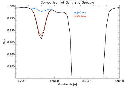
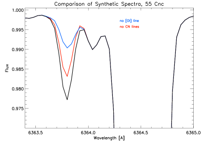
Figure 1: Top row: The contribution of CN to the blended 6363 Å [O I] line is greater in 55 Cnc than in a solar-type star. The black line shows the model spectrum of (left) the sun and (right) 55 Cnc with our adopted stellar paraemters. In red is the stellar model with CN lines removed, showing the contribution of just [O I]. In blue is the stellar model with the [O I] line removed, showing the contribution of just the CN lines. Bottom: The measured log$N$(O)_55Cnc changes significantly within the error on the determined log$N$(Ni) abundance (log$N$(Ni)${}_{\rm{55Cnc}}=$6.68$\pm$0.05).

However, as noted above, this line is blended with Ni and we find that in 55 Cnc, the derived [O/H]₆₃₀₀ is very sensitive to the assumed abundance of nickel when performing synthesis analysis. By changing the Ni abundance within our derived error for [Ni/H] ($\pm$0.05), the best-fit oxygen abundance log$N$(O) varies by $\sim$0.20 (see Figure 1, bottom). This results in the C/O ratio varying from $\sim$0.72-1.1, without even considering the 1$\sigma$ C/O errors (and $\sim$0.42-1.4 considering these errors).

The [O I] 6363.78 Å line gives a C/O$=$0.79$\pm$0.23, ranging within error from $\sim$solar (C/O_⊙=0.55$\pm$0.10; Asplund et al. 2009; Caffau et al. 2011) to 1. This line is a blend with CN, which we find contributes a greater amount to the line strength in the case of 55 Cnc than in the Sun (see Figure 1, top). Additionally, it is weaker than the [O I] 6300 Å line, and was found to give higher oxygen abundances in the Sun (e.g., log$N$(O)₆₃₀₀=8.69 vs. log$N$(O)₆₃₆₃=8.81), 2 dwarf stars, and a sub-giant star (Caffau et al. 2008; Caffau et al. 2013). (We find log$N$(O)_⊙,6300=8.67 vs. log$N$(O)_⊙,6363=8.84 in our synthesis analysis of the Sun.) Caffau et al. (2013) suggest that the discrepancy is due to an overestimate in the log $gf$ of the Ni I line that is blended with the [O I] 6300.30 Å line. Alternatively, an unknown blend at 6363 Å may affect the spectrum of dwarf stars only, as the 6300-6363 Å discrepancy is not seen in giants (Caffau et al. 2013). Certainly this discussion is still open, and this particular result should be considered as part of a larger effort to determine [O/H] from both [O I] lines in dwarf star spectra. Overall, because [O/H]₆₃₆₃ for 55 Cnc is larger, the resulting C/O is smaller than for the 6300 Å line.

For the O I triplet at 7771-7775 Å, the LTE [O/H]${}_{\rm{LTE}}=$0.19$\pm$0.17 agrees well with that derived from the [O I] 6363.78 Å, 0.17$\pm$0.17, resulting in a similar C/O$=$0.76$\pm$0.23. As noted, these lines have been shown both theoretically and observationally to overestimate oxygen abundances in LTE, most significantly at high temperatures and low gravities. We show in Tables 3 and 4 that three different NLTE corrections – Takeda (2003), Ramírez et al. (2007), and Fabbian et al. (2009) – give different [O/H] values and C/O ratios for 55 Cnc. The corrections are relatively small and, perhaps surprisingly, similar despite the different atomic models, handling of H atom inelastic collisions, and stellar parameters covered by the corrections. For varying NLTE corrections, C/O_55Cnc ranges from $\sim$0.63-0.70, with a conservative error of $\sim$0.2 based on the LTE abundances (see §2.5).

However, we note that the validity of applying these NLTE corrections to a cool and metal-rich star like 55 Cnc is uncertain. With high-resolution spectroscopy and analysis methods very similar to those used here, Schuler et al. (2004) and (2006) and King & Schuler (2005) find a significant $increase$ [O/H]_LTE values derived from the O I triplet with $decreasing$ $T_{\rm{eff}}$ for dwarfs stars in the Pleiades, M34, Hyades open clusters, and the Ursa Major moving group. Such collections of stars present a unique opportunity for studying the NLTE effects across stellar temperature and thus mass, as the stars are presumably, within a single cluster, chemically homogenous and formed at the same time. This increase in [O/H]_LTE is in direct contrast with all the NLTE calculations presented here, which predict negligible effects (e.g., $\leq$ 0.05 dex) in dwarfs with $T_{\rm{eff}}\lesssim$5400 K. These cool cluster dwarf findings are robust, in that the trend remains after re-derivation of temperatures using different (e.g., photometric) scales, across multiple stellar atmosphere models with or without convective treatment and varying the mixing-length parameter, and within all four of these stellar associations.

The physical mechanism responsible for the discrepancy in triplet oxygen abundances between calculations and observations of cool ($T_{\rm{eff}}\lesssim$5400 K) dwarfs in clusters is not yet certain. By comparing the Hyades cluster (600 Myr; [Fe/H]=+0.13), Pleiades cluster ($\sim$100 Myr, [Fe/H]=0), and Ursa Major moving group (600 Myr, [Fe/H]=-0.09), Schuler et al. (2006) suggest that the similarity in the observed [O/H]-$T_{\rm{eff}}$ trend in Hyades and Ursa Major, versus the steeper trend in Pleiades, points towards an age rather than metallicity effect. While the line strengths of the triplet have been shown to increase in a synthetic solar spectrum when a chromosphere is included (Takeda 1995), Schuler et al. (2004) find no correlation between the triplet [O/H] values and H$\alpha$ and Ca II triplet chromospheric activity indicators for the Pleiades and M34 stars. This lack of correlation is confirmed by Schuler et al. (2006) between the Hyades stars’ [O/H] and Ca II H+K activity indicators, suggesting that a more global chromosphere does not contribute to the observed triplet trends in cool cluster dwarfs. Instead, using simple models including flux contributions to the triplet region from the quiescent star and both cool and hot spots is, Schuler et al. (2006) are able to reproduce the observed oxygen triplet line strengths in cool Hyades dwarfs. As stellar surface activity is expected to decrease with age, this result is consistent with the suspected age dependence of the cool star O I triplet abundances.

Our derived $T_{\rm{eff}}$ for 55 Cnc (5350$\pm$102 K) places it in the regime ($T_{\rm{eff}}\lesssim$ 5450 K) where the O I triplet-temperature trend appears to contradict the canonicial NLTE oxygen abundance corrections. Due to the larger oxygen triplet NLTE correction in the Sun versus 55 Cnc, the resulting NLTE-corrected [O/H] values for 55 Cnc are actually larger than [O/H]_LTE, although overlap within errors (see Table 3). This behavior is also seen in the cooler stars of Nissen (2013) – NLTE corrections in cool stars (even up to $\sim$5660 K) yield an increase in [O/H]. As a result of higher oxygen abundances, the C/O ratios for 55 Cnc derived here using the various [O/H]_NLTE values are smaller, with a mean of 0.66$\pm$0.07 using the averaged log$N$(C) of the two [C/H] indicators. However, all of the stellar associations discussed above are much younger than the estimated age of 55 Cnc (2-6 Gyr), so the same mechanism(s) may not apply in this case.

Instead of adopting the canonical NLTE corrections, one could estimate an empirical correction based on the open cluster and moving group data from Schuler et al. (2006). At 5350 K, the T_eff of 55 Cnc, the typical O I triplet-based abundances are approximately 0.08 dex higher than the mean abundances of the warmer stars in each cluster. Adopting this difference as a first-order correction, the resulting O I triplet abundance of 55 Cnc would be [O/H] = 0.11, a value in good agreement with the [O I]-based abundances.

Table 4 presents final abundances and respective C/O ratios from the individual C I, C₂, [O I], and O I triplet features. As discussed earlier, at the temperature and metallicity of 55 Cnc, the 6300Å [O I] feature is dominated by the Ni I blend. Inspection of the O-results in Table 4 reveals that the 6300Å line yields a lower [O/H] than the other oxygen indicators. A mean of the O I triplet LTE and the 6363Å [O I] line results in log$N$(O)=8.84$\pm$0.01; the 6300Å [O I] abundance falls significantly outside of this scatter at log$N$(O)=8.74. The decision here, due to uncertainty caused by significant Ni I blending, is to drop the 6300Å [O I] result from the final C/O calculation. Additionally, the various NLTE corrections to the O I triplet abundance may be unreliable at the temperature and metallicity of 55 Cnc. The O I triplet NLTE log$N$(O)=8.91$\pm$0.027, different by $\sim$1.9$\sigma$ from the log$N$(O)=8.84$\pm$0.01 calculated from the combined 6363Å [O I] line and O I triplet LTE values. Therefore we also omit the triplet NLTE results from the final C/O calculation. We note, though, that including the triplet NLTE values decreases the mean C/O value only slightly, to 0.71$\pm$0.09, in agreement with the value we choose to report based on the 6363Å [O I] and O I triplet LTE values. In addition, including the O I triplet LTE values with the empirical correction derived from the cool cluster stars increases the mean C/O value slightly ($\sim$0.03 dex) but is completely consistent with the average we choose to report here.

A final mean C/O ratio is calculated for 55 Cnc based on the six values of C/O in Table 4, which result from each combination of values from each respective C and O abundance indicator, excluding those based on the 6300Å [O I] line and the O I triplet NLTE corrections. The resulting mean value is C/O=0.78$\pm$0.08. Precise values of C/O are important for constraining the composition of this multiple-planet host star. Several other studies are tackling this issue with larger samples of mostly giant planet host stars (Delgado Mena et al. 2010; Petigura & Marcy 2011; Nissen 2013).

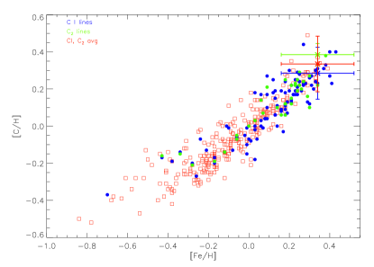
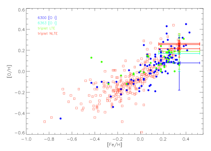
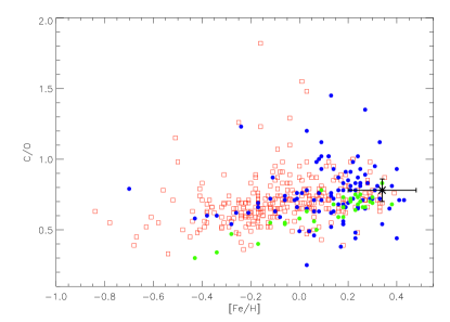
Figure 2: [C/H], [O/H], and C/O versus [Fe/H] from Delgado Mena et al. (2010) and Nissen (2013) [all Nissen (2013) hosts are in the Delgado Mena et al. (2010) host sample]. Non-host stars from Delgado Mena et al. (2010) are plotted with red open squares, while host stars from Delgado Mena et al. (2010)/Nissen (2013) are plotted with blue/green circles. Measurements of 55 Cnc from this work are represented by large asterisks in each plot (see Table 3). In the upper plots, we designate measurements from different C and O abundance indicators with different colors. Our final mean C/O value is shown in black in the bottom plot.

Figure 2 shows the values of [C/H], [O/H], and C/O versus [Fe/H] for stars from the samples noted in the previous paragraph, with the results derived here for 55 Cnc also shown. While the spread is still large, the bottom panel of Figure 2 showing C/O versus [Fe/H] indicates that 55 Cnc follows the same trends as defined by the larger samples. With C/O=0.78$\pm$0.08, 55 Cnc exhibits a ratio that is significantly larger than solar (C/O${}_{\odot}\sim$0.50), but below C/O=1.0 at the 2.75$\sigma$ level. The value of 0.78 is lower than the value of C/O=1.12$\pm$0.19 used by Madhusudhan et al. (2012) for their carbon-rich models of the “super-Earth” exoplanet.

4 Conclusions

The 55 Cnc system was the first (Wisdom 2005) and remains one of only a few discovered systems with five or more planets.The inner most planet, 55 Cnc e, is one of the most observationally-favorable super-Earth exoplanets for detailed characterization.

While previous analyses indicate the C/O ratio of 55 Cnc to be $\geq$1, our analysis indicates that the picture is not so clear. The C/O ratio of this exoplanet host star is likely closer to $\sim$0.8. This value is lower than the value adopted by Madhusudhan et al. (2012) in their prediction that the small-mass exoplanet 55 Cnc e is carbon-rich, and corresponds to the predicted minimum value, $\sim$0.8, necessary to form abundant carbon-rich condensates, under the assumption of equilibrium (e.g., Bond et al. 2010). Also, possibly the C/O ratio of 55 Cnc’s protoplanetary disk was not uniformly identical to its host star, perhaps causing local carbon enhancements of the gas or grains accreted by 55 Cnc e; carbon-rich planets may still form around oxygen-rich stars (Öberg et al. 2011; Bond et al. 2010). Our study places this system at the theoretically interesting boundary between two diverse planetary types.

Measurements of oxygen are challenging in solar-type stars because the oxygen abundance indicators at optical wavelengths are weak, blended with other atomic or molecular lines, and/or subject to non-LTE effects. Oxygen measurements are even more complicated in cool and high metallicity stars like 55 Cnc, because of the stronger blends with both atomic and molecular lines, and the uncertainty in NLTE corrections that do not accurately predict the behavior of line widths in cool stars. Our case study demonstrates the caution that must be used when determining exoplanet host star (and any star’s) C/O ratios, particularly the sensitivity of all three major oxygen abundance indicators to different effects that are not always easy to account for and change based on stellar parameters.

Table 1: Derived Stellar Parameters and Elemental Abundances for 55 Cnc

Parameter	this worka	Valenti & Fischer 2005b	Butler et al. 2006	Ecuvillon et al. 2004 or 2006	Takeda et al. 2007	Zielinski et al. 2012
$T_{\rm{eff}}$ (K)	5350$\pm$102	5235$\pm$15	5235$\pm$44	5279$\pm$62	5327$\pm$49	5265$\pm$15
log $g$ (cgs)	4.44$\pm$0.30	4.45$\pm$0.02	4.45$\pm$0.06	4.37$\pm$0.18	4.48${}^{-0.01}_{+0.05}$	4.49$\pm$0.05
$\xi$ (km s-1)	1.17$\pm$0.14	$\cdots$	$\cdots$	0.98$\pm$0.07	$\cdots$	$\cdots$
[Fe/H]	0.34$\pm$0.18	0.31$\pm$0.01	0.32$\pm$0.03	0.33$\pm$0.07	0.37$\pm$0.04	0.29$\pm$0.07
[Ni/H]	0.43$\pm$0.05	0.37$\pm$0.01	$\cdots$	0.39c	$\cdots$	$\cdots$

Table 2: Lines Measured, Equivalent Widths, and Abundances

Ion	$\lambda$	$\chi$	log $gf$	EW⊙	log$N_{\odot}$	EW55Cnc	log$N_{\rm{55Cnc}}$
	(Å)	(eV)		(mÅ)		(mÅ)
C I	5052.17	7.68	-1.304	33.7	8.45	31.3	8.72
	5380.34	7.68	-1.615	20.7	8.48	20.6	8.78
$[$O I$]$	6300.30	0.00	-9.717	5.6	8.67a	7.2	8.75a
	6363.79	0.00	-10.185	1.6	8.84a	3.4	9.01a
O I	7771.94	9.15	0.369	69.6	8.83	48.9	9.00
	7775.39	9.15	0.001	46.8	8.81	33.6	9.01

Note. — This table is available in its entirety in a machine-readable form in the online journal. A portion is shown here for guidance regarding its form and content.

Table 3: 55 Cnc Carbon and Oxygen Abundances from Different Indicators

Abundance Indicator	this worka	Ecuvillon et al. 2004 or 2006b	Delgado Mena et al. 2010c	Petigura & Marcy 2011d
[C I/H]	0.29$\pm$0.14	0.31$\pm$0.10	0.30	0.13$\pm$0.06
[C2/H]	0.39$\pm$0.06	$\cdots$	$\cdots$	$\cdots$
[O/H]6300	0.08$\pm$0.26	0.13$\pm$0.11	0.07	$\cdots$
[O/H]6363	0.17$\pm$0.17	$\cdots$	$\cdots$	$\cdots$
[O/H]7772,7775;LTE	0.19$\pm$0.17	0.21${}_{\rm{no\,LTE\,error\,given}}^{\rm{avg\,of\,all\,triplet\,lines}}$	$\cdots$	$\cdots$
[O/H]7772,7775;NLTE	0.22$\pm$0.08${}_{\rm{Takeda\,NLTE}}$	0.03$\pm$0.11${}_{\rm{Ecuvillon\,NLTE\,model}}^{\rm{avg\,of\,all\,triplet\,lines}}$	$\cdots$	$\cdots$
	0.25$\pm$0.03${}_{\rm{Ramirez\,NLTE}}$
	0.27$\pm$0.03${}_{\rm{Fabbian\,NLTE}}$

Note. — The NLTE corrections calculated from Fabbian et al. (2009) have been interpolated to a Drawin formula scaling factor S${}_{\rm{H}}=0.85$, as in Nissen 2013.

Table 4: C/O Ratios of 55 Cnc Based on Different C and O Abundance Indicators

	log$N$(O)	6300 Å [O I]	O I triplet	O I triplet	O I triplet	O I triplet	6363 Å [O I]
		log$N$(Ni)=6.68	LTE	NLTE Takeda (2003)	NLTE Ramírez et al. (2007)	NLTE Fabbian et al. (2009)
log$N$(C)		8.740	8.845	8.875	8.915	8.926	8.830
two blue C I lines	8.675	0.861$\pm$0.299	0.676$\pm$0.217	0.631$\pm$0.217	0.576$\pm$0.217	0.561$\pm$0.217	0.700$\pm$0.217
two C2 lines	8.775	1.084$\pm$0.272	0.851$\pm$0.178	0.794$\pm$0.178	0.725$\pm$0.178	0.706$\pm$0.178	0.881$\pm$0.178
C I and C2 averaged	8.725	0.966$\pm$0.306	0.759$\pm$0.226	0.707$\pm$0.226	0.646$\pm$0.226	0.629$\pm$0.226	0.785$\pm$0.226

Note. — The log$N$(O or C) values are calculated as [X/H]$+$log$N_{\odot}$(X), with log$N_{\odot}$(O)=8.66 and log$N_{\odot}$(C)=8.39 (Asplund et al. 2005). The $\pm$ errors here $=$ the final combined abundance uncertainties due to both stellar parameters and (if applicable) the dispersion in abundances derived from multiple lines. We adopted the more conservative (larger) [O/H]_LTE errors for the [O/H]_NLTE values. Serendipitously, the [O/H]_LTE error $=$ the [O I]₆₃₆₃ error; hence, columns 4-8 have identical errors.

References

- Allende Prieto et al. (2003) Allende Prieto, C., Hubeny, I., & Lambert, D. L. 2003, ApJ, 591, 1192
- Asplund et al. (2005) Asplund, M., Grevesse, N., & Sauval, A. J. 2005, Cosmic Abundances as Records of Stellar Evolution and Nucleosynthesis, 336, 25
- Asplund et al. (2004) Asplund, M., Grevesse, N., Sauval, A. J., Allende Prieto, C., & Kiselman, D. 2004, A&A, 417, 751
- Baliunas et al. (1997) Baliunas, S. L., Henry, G. W., Donahue, R. A., Fekel, F. C., & Soon, W. H. 1997, ApJ, 474, L119
- Barklem (2007) Barklem, P. S. 2007, A&A, 462, 781
- Bensby et al. (2005) Bensby, T., Feltzing, S., Lundström, I., & Ilyin, I. 2005, A&A, 433, 185
- Bensby et al. (2004) Bensby, T., Feltzing, S., & Lundström, I. 2004, A&A, 415, 155
- Bond et al. (2010) Bond, J. C., O’Brien, D. P., & Lauretta, D. S. 2010, ApJ, 715, 1050
- Borucki et al. (2011) Borucki, W. J., Koch, D. G., Basri, G., et al. 2011, ApJ, 736, 19
- Bubar & King (2010) Bubar, E. J., & King, J. R. 2010, AJ, 140, 293
- Caffau et al. (2011) Caffau, E., Ludwig, H.-G., Steffen, M., Freytag, B., & Bonifacio, P. 2011, Sol. Phys., 268, 255
- Caffau et al. (2013) Caffau, E., Ludwig, H.-G., Malherbe, J.-M., et al. 2013, A&A, 554, A126
- Caffau et al. (2008) Caffau, E., Ludwig, H.-G., Steffen, M., et al. 2008, A&A, 488, 1031
- Carter-Bond et al. (2012) Carter-Bond, J. C., O’Brien, D. P., Delgado Mena, E., et al. 2012, ApJ, 747, L2
- Cayrel de Strobel et al. (1999) Cayrel de Strobel, G., Lebreton, Y., Soubiran, C., & Friel, E. D. 1999, Ap&SS, 265, 345
- Cunha et al. (1998) Cunha, K., Smith, V. V., & Lambert, D. L. 1998, ApJ, 493, 195
- Delgado Mena et al. (2010) Delgado Mena, E., Israelian, G., González Hernández, J. I., Bond, J. C., Santos, N. C., Udry, S., Mayor, M., 2010, ApJ, 725, 2349
- Demory et al. (2011) Demory, B.-O., Gillon, M., Deming, D., et al. 2011, A&A, 533, A114
- Dragomir et al. (2013) Dragomir, D., Matthews, J. M., Winn, J. N., Rowe, J. F., & MOST Science Team 2013, arXiv:1302.3321
- Drawin (1968) Drawin, H.-W. 1968, Zeitschrift fur Physik, 211, 404
- Eggen (1985) Eggen, O. J. 1985, AJ, 90, 74
- Endl et al. (2012) Endl, M., Robertson, P., Cochran, W. D., et al. 2012, ApJ, 759, 19
- Fabbian et al. (2009) Fabbian, D., Asplund, M., Barklem, P. S., Carlsson, M., & Kiselman, D. 2009, A&A, 500, 1221
- Feltzing & Gonzalez (2001) Feltzing, S., & Gonzalez, G. 2001, A&A, 367, 253
- Fitzpatrick & Sneden (1987) Fitzpatrick, M. J., & Sneden, C. 1987, BAAS, 19, 1129
- Fortney (2012) Fortney, J. J. 2012, ApJ, 747, L27
- Fuhrmann et al. (1998) Fuhrmann, K., Pfeiffer, M. J., & Bernkopf, J. 1998, A&A, 336, 942
- Gillon et al. (2012) Gillon, M., Demory, B.-O., Benneke, B., et al. 2012, A&A, 539, A28
- Gonzalez (1999) Gonzalez, G. 1999, MNRAS, 308, 447
- Gonzalez & Vanture (1998) Gonzalez, G., & Vanture, A. D. 1998, A&A, 339, L29
- Gratton et al. (1999) Gratton, R. G., Carretta, E., Eriksson, K., & Gustafsson, B. 1999, A&A, 350, 955
- Hibbert et al. (1991) Hibbert, A., Biemont, E., Godefroid, M., & Vaeck, N. 1991, Journal of Physics B Atomic Molecular Physics, 24, 3943
- Hibbert et al. (1993) Hibbert, A., Biemont, E., Godefroid, M., & Vaeck, N. 1993, A&AS, 99, 179
- Hubeny & Lanz (1995) Hubeny, I., & Lanz, T. 1995, ApJ, 439, 875
- Johnson et al. (2012) Johnson, T. V., Mousis, O., Lunine, J. I., & Madhusudhan, N. 2012, ApJ, 757, 192
- King & Schuler (2005) King, J. R., & Schuler, S. C. 2005, PASP, 117, 911
- Kiselman (1991) Kiselman, D. 1991, A&A, 245, L9
- Kiselman (1993) Kiselman, D. 1993, A&A, 275, 269
- Kurucz (1993) Kurucz, R. 1993, Opacities for Stellar Atmospheres: Abundance Sampler. Kurucz CD-ROM No. 14. Cambridge, Mass.: Smithsonian Astrophysical Observatory, 1993., 14,
- Kurucz & Bell (1995) Kurucz, R., & Bell, B. 1995, Atomic Line Data (R.L. Kurucz and B. Bell) Kurucz CD-ROM No. 23. Cambridge, Mass.: Smithsonian Astrophysical Observatory, 1995., 23,
- Kuchner & Seager (2005) Kuchner, M. J., & Seager, S. 2005, arXiv:astro-ph/0504214
- Kupka et al. (1999) Kupka, F., Piskunov, N., Ryabchikova, T. A., Stempels, H. C., & Weiss, W. W. 1999, A&AS, 138, 119
- Lambert & Ries (1981) Lambert, D. L., & Ries, L. M. 1981, ApJ, 248, 228
- Lovis et al. (2009) Lovis, C., Mayor, M., Bouchy, F., et al. 2009, IAU Symposium, 253, 502
- Madhusudhan et al. (2012) Madhusudhan, N., Lee, K. K. M., & Mousis, O. 2012, ApJ, 759, L40
- McArthur et al. (2004) McArthur, B. E., Endl, M., Cochran, W. D., et al. 2004, ApJ, 614, L81
- Nissen (2013) Nissen, P. E. 2013, A&A, 552, A73
- Öberg et al. (2011) Öberg, K. I., Murray-Clay, R., & Bergin, E. A. 2011, ApJ, 743, L16
- Pereira et al. (2009) Pereira, T. M. D., Asplund, M., & Kiselman, D. 2009, A&A, 508, 1403
- Petigura & Marcy (2011) Petigura, E. A., & Marcy, G. W. 2011, ApJ, 735, 41
- Ramírez et al. (2007) Ramírez, I., Allende Prieto, C., & Lambert, D. L. 2007, A&A, 465, 271
- Schuler et al. (2011) Schuler, S. C., Flateau, D., Cunha, K., King, J. R., Ghezzi, L., Smith, V. V., 2011, ApJ, 732, 55
- Schuler et al. (2004) Schuler, S. C., King, J. R., Hobbs, L. M., & Pinsonneault, M. H. 2004, ApJ, 602, L117
- Schuler et al. (2006) Schuler, S. C., King, J. R., Terndrup, D. M., et al. 2006, ApJ, 636, 432
- Sneden (1973) Sneden, C. 1973, ApJ, 184, 839
- Steenbock & Holweger (1984) Steenbock, W., & Holweger, H. 1984, A&A, 130, 319
- Storey & Zeippen (2000) Storey, P. J., & Zeippen, C. J. 2000, MNRAS, 312, 813
- Sumi et al. (2010) Sumi, T., Bennett, D. P., Bond, I. A., et al. 2010, ApJ, 710, 1641
- Takeda (1995) Takeda, Y. 1995, PASJ, 47, 463
- Takeda (2003) Takeda, Y. 2003, A&A, 402, 343
- Takeda & Honda (2005) Takeda, Y., & Honda, S. 2005, PASJ, 57, 65
- Taylor (2002) Taylor, B. J. 2002, MNRAS, 329, 839
- Teske et al. (2013) Teske, J. K., Schuler, S. C., Cunha, K., Smith, V. V., & Griffith, C. A. 2013, ApJ, 768, L12 Urdahl, R. S., Bao, Y., & Jackson, W. M. 1991, Chemical Physics Letters, 178, 425
- van Leeuwen (2007) Van Leeuwen, F. 2007, A&A, 474, 653
- Vogt et al. (1994) Vogt, S. S., Allen, S. L., Bigelow, B. C., et al. 1994, Proc. SPIE, 2198, 362
- Winn et al. (2011) Winn, J. N., Matthews, J. M., Dawson, R. I., et al. 2011, ApJ, 737, L18
- Wisdom (2005) Wisdom, J. 2005, Bulletin of the American Astronomical Society, 37, 525