Published in HELIUM THREE
Volume 26 of Modern Problems in Condensed Matter Physics, Chapter 5, pp. 255–311.
Edited by W. P. Halperin and L. P. Pitaevskii, North-Holland, 1990.

Collective Modes and Nonlinear Acoustics in

Superfluid ³He-B

Ross H. McKenzie^† and J. A. Sauls

Department of Physics and Astronomy

Northwestern University

2145 Sheridan Road

Evanston, Illinois 60208

April 1990

^†Current address: Department of Physics, Ohio State University, Columbus, OH 43210.

5.1 Introduction

Ultrasound has been used extensively to study the collective excitations in superfluid ³He. Early ultrasonic studies of order parameter collective modes provided important confirmation of the identifications of the A- and B-phases based on NMR. More recent experimental studies have discovered a remarkable spectrum of order parameter collective modes that clearly reveal the underlying broken symmetries of the superfluid phases. Theoretical studies have further elucidated the nature of the collective modes in terms of the condensate of Cooper pairs and their couplings to external fields, quantified the energy spectrum and underlying molecular fields of the Fermi liquid, and predicted a number of new physical effects, many of which have striking similarities to the interaction of electromagnetic fields with the atoms and molecules. The article by Halperin and Varoquaux [26] in this volume gives a comprehensive review of ultrasonic experiments in superfluid ³He as well as their theoretical interpretation in terms of collective modes of the order parameter. Most studies of collective modes in superfluid ³He have delt with the linear response of the condensate. In this article we present recent theoretical work on the role of order parameter collective modes in the nonlinear response of ³He-B to acoustic waves. Many of the nonlinear acoustic phenomena we describe have analogs in nonlinear optical excitation of atoms and molecules.

The subject of order parameter collective modes originated with questions that were raised about the gauge invariance of the original BCS theory [3]. Anderson [4] provided a gauge-invariant formulation of the pairing theory and elucidated the role of collective modes in superconductors (see also [54, 50, 2]). These modes may be broadly classified into (i) Goldstone modes, associated with a spontaneously broken symmetry, and (ii) exciton modes, excitations of the condensate of Cooper pairs which involve time-dependent deformation of the superconducting order parameter [42]. Goldstone modes reflect the degeneracy of the order parameter under time-independent and spatially uniform gauge transformations and rotations, and are the low-energy excitations of the condensate. Broken gauge symmetry in superconductors and superfluid ³He leads to a phase mode, oscillations in the overall phase of the order parameter. This mode is closely related to the collisionless sound mode in superfluid ³He and exhibits a phonon-like dispersion relation, $\omega=c_{1}q$, where the velocity $c_{1}$, in the limit $T\rightarrow 0$ and $\omega\ll\Delta$, is identical to the hydrodynamic sound velocity of the normal phase of liquid ³He. The phase mode was predicted by Anderson [4] and Bogoliubov, Tolmachev and Shirkov [11], and is essential to spectroscopic studies of the additional order parameter collective modes in ³He. Several authors also predicted the existence of exciton modes in superconductors with excitation energies, $\omega<2\Delta$, corresponding to excited bound states of Cooper pairs [4, 11, 70, 71, 8]. Most notable from the viewpoint of collective modes in superfluid ³He is the work of Vdovin [72] who predicted the order parameter collective modes for the Balian-Werthamer state, and calculated the dispersion relations, long before the discovery of superfluid ³He. Although exciton modes have never been definitively observed in superconductors to our knowledge, the analogous modes in superfluid ³He have been studied extensively. The main reason that exciton modes are readily observed in superfluid ³He, while not in most superconductors, is that ³He is an unconventional superfluid with an order parameter that breaks the rotational invariance in both spin- and orbital space; and therefore, belongs to a higher dimensional representation of the full symmetry group of the normal phase. This implies that there is a spectrum of pairing states - the ground pair state and excited pair states - belonging to the same representation, and therefore bound by the same pairing interaction. It is well established that the superfluid phases of ³He belong to the $S=1,\ l=1$ (spin-triplet, p-wave) representation of the rotation group $SO(3)\times SO(3)$, giving rise to an order parameter with nine complex amplitudes and a corresponding spectrum of eighteen collective modes, many of which lie well below the pair-breaking edge of $2\Delta$.

Quite generally the order parameter can be identified as the pair amplitude,

$$F_{\alpha\beta}({\bm{r}},{\bm{x}})=\langle\psi_{\alpha}({\bm{x}}+{\bm{r}}/2)\psi_{\beta}({\bm{x}}-{\bm{r}}/2)\rangle\;.$$ (5.1)

Since pairing occurs in a narrow band in momentum space near the Fermi momentum, $p_{f}$, it is convenient to use a mixed Fourier-space representation,

$$F_{\alpha\beta}({\bm{p}},{\bm{x}})=\int\limits d^{3}r\,e^{-i{\bm{p}}\cdot{\bm{r}}}\,F_{\alpha\beta}({\bm{r}},{\bm{x}})\;,$$ (5.2)

with $|{\bm{p}}|\simeq p_{f}$. Thus, $F_{\alpha\beta}({\bm{p}},{\bm{x}})\simeq F_{\alpha\beta}(p_{f}\hat{\bm{p}},{\bm{x}})$ is a function of the center-of-mass coordinate, ${\bm{x}}$, of the Cooper pair for non-uniform states of the superfluid, and the direction $\hat{\bm{p}}$ describes the orbital motion of the pair. In addition, the order parameter depends on the spin configuration $(\alpha,\beta)$ of the Cooper pairs, and can be decomposed into spin-singlet $(S=0)$ and spin-triplet $(S=1)$ amplitudes,

$$F_{\alpha\beta}(\hat{\bm{p}})=f_{0}(\hat{\bm{p}})(i\sigma_{y})_{\alpha\beta}+{\bm{f}}(\hat{\bm{p}})\cdot(i{\bm{\sigma}}\sigma_{y})_{\alpha\beta}\;,$$ (5.3)

where ${\bm{f}}(\hat{\bm{p}})$ represents the three odd-parity, spin-triplet amplitudes. In equilibrium the superfluid phases of ³He are described by an order parameter in which only the spin-triplet part is non-zero. The rotational invariance of the normal phase of ³He suggests that the condensate of Cooper pairs is also defined by a single orbital angular momentum channel, known to be the p-wave channel. An alternative order parameter to the pair field, ${\bm{f}}({\bm{x}},\hat{\bm{p}})$, is the weak-coupling gap function,

$${\bm{\Delta}}({\bm{x}},\hat{\bm{p}})=\int\frac{d\Omega^{\prime}}{4\pi}\;V^{t}(\hat{\bm{p}}\cdot\hat{\bm{p}}^{\prime})\;{\bm{f}}({\bm{x}},\hat{\bm{p}}^{\prime})\,,$$ (5.4)

where $V^{t}$ is the pairing interaction in the spin-triplet channel; for equilibrium states of ³He these two order parameters contain essentially the same information. A trivial extension of the above to include time-dependent pair amplitudes describes non-equilibrium states of the condensate described by a fluctuation of the order parameter,

$${\bm{d}}(\hat{\bm{p}};{\bm{x}},t)=\int\frac{d\Omega^{\prime}}{4\pi}\,V^{t}(\hat{\bm{p}}\cdot\hat{\bm{p}}^{\prime})\,\left[{\bm{f}}(\hat{\bm{p}}^{\prime};{\bm{x}},t)-{\bm{f}}_{eq}(\hat{\bm{p}}^{\prime})\right]\;,$$ (5.5)

where ${\bm{f}}(\hat{\bm{p}};{\bm{x}},t)$ is the time-dependent pair amplitude defined in Sec. (5.3).

The equilibrium B-phase is decribed by the an order parameter of the Balian-Werthamer (BW) class [7],

$$\Delta_{i}(\hat{\bm{p}})=\Delta(T)\,R_{i\alpha}[\hat{\bm{n}},\theta]\;e^{i\Phi}\;(\hat{\bm{p}})_{\alpha}\;,$$ (5.6)

where $R_{i\alpha}[\hat{\bm{n}},\theta]$ is an orthogonal matrix defining a relative rotation of the spin and orbital angular momentum quantization axes, $\Phi$ is the global phase, and $\Delta(T)$ is the magnitude of the gap. If we neglect the weak dipolar interaction then the free energy of ³He is separately invariant under spin rotations and orbital rotations. Thus, the BW states described by different relative rotations of the spin- and orbital coordinates are degenerate, as are BW states differing by a gauge transformation. The parameters $\left[\hat{\bm{n}},\theta,\Phi\right]$ that define the equilibrium B-phase order parameter are soft degrees of freedom; long-wavelength variations of these fields cost little energy on the scale of $T_{c}$. The nuclear dipolar interaction, which is small on the scale of $T_{c}\,(E_{dipolar}\sim 10^{-7}K\ll T_{c}\sim 10^{-3}K)$, partially lifts this degeneracy by fixing the rotation angle $\theta=\cos^{-1}(-1/4)$ [38]; but the direction of the axis of rotation $\hat{\bm{n}}$ remains a soft degree of freedom. Many of the remarkable properties of superfluid ³He are related to these soft degrees freedom and are described in detail elsewhere in this volume.

The B-phase, described by one of the the BW states, is “pseudo-isotropic” in the sense that it is invariant under the transformations generated by the total “twisted” angular momentum ${\bm{J}}={\bm{L}}+\mathop{\underline{R}}(\hat{\bm{n}},\theta)^{-1}\cdot{\bm{S}}$, and so has total “twisted angular momentum” $J=0$. For pure $l=1$ pairing the order parameter collective modes correspond to the natural oscillations of the $3\times 3$ complex matrix $D_{ij}({\bm{x}},t)$ defined in terms of the time-dependent order parameter for pairing fluctuations,

$$d_{i}(\hat{\bm{p}};{\bm{x}},t)=D_{ij}({\bm{x}},t)\hat{\bm{p}}_{j}\,.$$ (5.7)

The eighteen order parameter modes are classified [40] by the quantum numbers $J^{\zeta}$ and $M$, where $J=\{0,1,2\}$ is the total angular momentum, $M=\{-J,\ldots,0,\ldots+J\}$ is the magnetic quantum number, and $\zeta=\{+,-\}$ is the signature of the pair amplitude under the particle-hole transformation. The $J=2^{+}$ and $J=2^{-}$ modes are of particular interest because they have excitation energies which lie well below the pair-breaking edge of $2\Delta(T)$ [$\omega_{2^{+}}\simeq 1.1\;\Delta(T)$ and $\omega_{2^{-}}\simeq 1.5\;\Delta(T)$], couple to sound and are only weakly damped by quasiparticles collisions. The linear interaction of zero sound with the order parameter collective modes of ³He for frequencies in the range of $10-100$ MHz has a number of similarities with the interaction of light with atoms, molecules and solids, including:

• a spectroscopic classification of modes (excited states) in terms of quantum numbers for rotational and discrete symmetries,

• sharp resonance features in the phase velocity, group velocity and attenuation of sound (light) when its frequency and wave-vector matches that of the collective modes (excited states),

• a linear Zeeman splitting of the collective modes (excited states) in magnetic field, and

• a nonlinear splitting of modes (excited states) in large magnetic fields due in part to level repulsion.

Partly because of the similarities between the ultrasonic absorption spectrum of superfluid ³He and optical systems, as well as the sharpness of the collective mode resonances, ³He is an ideal media in which to look for acoustic analogues of nonlinear optical effects.

Nonlinear optical effects can be broadly divided into two classes. One class of effects occur because intense radiation induces a macroscopic population of one or more of the excited states of the medium. Consequently, the occupation of the ground state of the system must be included as a dynamical variable in the constitutive equations. Examples include population inversion, saturation effects and self-induced transparency [1]. A second class of nonlinear effects are parametric processes such as harmonic generation, stimulated Raman scattering and two-photon absorption [10, 76]. Usually the population of the ground state need not be treated as a dynamical variable and can be assumed to have its equilibrium value. Except for a theoretical paper by Serene [65] on third-harmonic generation, previous investigations, both experimental and theoretical, of nonlinear sound in superfluid ³He have all involved effects belonging to the first class above. We briefly review these before turning to the main subject of this article, parametric processes.

Polturak et al. [51] observed saturation of the attenuation of zero sound in ³He-B for frequencies nearly resonant with the $J=2^{+}$ mode, as well as propagation delay, pulse sharpening and break-up of narrow sound pulses. They pointed out that these observations were qualitatively similar to self-induced transparency. Sauls [56] constructed a phenomenological set of nonlinear equations, which are consistent with the symmetries of superfluid ³He-B, reduce to the known linear equations, and are analogous to the Maxwell-Bloch equations for the optical self-induced transparency. He found that the relationship between the pulse width and the pulse velocity for the soliton solutions of these equations was in good agreement with the results of Polturak et al. However, Rouff and Varoquaux [55] questioned the interpretation of the experiments of Polturak, et al. in terms of self-induced transparency and pointed out that the energy density required for the formation of solitons in Sauls’ phenomenological theory, which is of the order of the superfluid condensation energy density, is two orders of magnitude larger than the estimated energy density in the sound pulses of Polturak et al. The discrepancy with the energy density of the phenomenological theory, combined with the observation of soliton-like propagation, underscores the need for a more fundamental theory of nonlinear sound propagation in superfluid ³He as well as further experimental efforts to study the nonlinear dynamics of the order parameter.

Nonlinear effects in the A-phase have also been observed. The attenuation of low-frequency zero sound in the ³He-A is dominated by the pair-breaking process near the nodes of the anisotropic energy gap. Avenel et al. [5] observed a decrease in the attenuation as the sound intensity was increased and showed that the reduction was due to a saturation effect from the creation of a non-equilibrium distribution of quasiparticles over a small region of the Fermi surface. Kopp and Wölfle [34] have recently derived dynamical equations for the quasiparticle distribution function, similar to the Maxwell-Bloch equations of nonlinear optics, which they use to describe the observations reported by Avenel et al [5].

Parametric processes, involving the absorption and emission of excitations with differing frequencies, are common in nonlinear systems and occur in diverse fields such as optics [68], plasma physics [27], electronics [77], and acoustics [13]. The simplest parametric process is a three-wave resonance in which nonlinear interactions allow two modes with frequencies $\omega_{1}$ and $\omega_{2}$ and wavevectors ${\bm{q}}_{1}$ and ${\bm{q}}_{2}$ to excite a third mode with frequency $\omega_{3}$ and wavevector ${\bm{q}}_{3}$ given by

$$\omega_{3}=\omega_{1}+\omega_{2}\,,\qquad{\bm{q}}_{3}={\bm{q}}_{1}+{\bm{q}}_{2}\,.\vspace*{-2mm}$$ (5.8)

Often the first wave, known as the pump wave, is of high intensity. The other waves are known as the idler and signal waves. The rate at which the process occurs depends on the intensity of the pump wave. The reverse process, the excitation of modes $1$ and $2$ by mode $3$, is also allowed. Such a parametric process is interpreted as the decay of a quanta of mode 3 into quanta of modes $1$ and $2$, and Eq. (5.8) expresses the conservation of energy and momentum. In Sec. (5.6) we discuss two particular parametric processes:

1. the production of a real squashon by two zero-sound phonons (two phonon absorption),

2. the decay of a zero-sound phonon into a real squashon and a second zero-sound phonon (stimulated Raman scattering).

Other processes such as third harmonic generation are discussed as extensions of the above two processes in Sec. (5.7).

Two important questions need to be answered by a theory of parametric processes in superfluid ³He:

1. When is a particular parametric process forbidden by the symmetry of the ground state of ³He, i.e. what are the selection rules?

2. What energy density of the pump wave is required for experimental detection of parametric excitation of the modes?

Liquid ³He possesses a number of symmetries and approximate symmetries, which determine the selection rules for parametric processes that occur. An example is the decay process for zero sound in normal ³He proposed by Ketterson [29] in which a zero-sound phonon decays into a spin wave by absorbing a $q=0$ magnon from a macroscopic population of such magnons that have been prepared by tipping the magnetization relative to the static field with an rf-pulse. However, such a decay process is not allowed [57], without dipolar interactions, because of the nearly exact invariance of the density matrix under separate rotations in spin and position space. Similarly, Serene [64] has shown that the approximate particle-hole symmetry of the ³He Fermi liquid determines important selection rules for the linear coupling of zero sound to the order parameter collective modes in superfluid ³He. This symmetry also determines important selection rules for parametric processes involving zero sound as discussed in Secs. (5.2) and (5.5). In fact because of particle-hole symmetry processes (1) and (2) above are allowed only for real squashons ($J=2^{+}$), not imaginary squashons ($J=2^{-}$). In Sec. (5.6) we discuss the coupling strengths of real squashons to sound via parametric processes and argue that the three-wave processes should be observable when the pump-wave energy density is of the order of the superfluid condensation energy density. Finally, in Sec. (5.7) we show that although the generation of third harmonics and anti-stokes waves are limited by dispersion, they may still be observable, at least for sufficiently short sound path lengths.

Section (5.3) is a review of the quasiclassical theory of superfluid ³He which provides the basis for our treatment of sound propagation and collective modes in the B-phase starting with the linear response theory in Sec. (5.4). These results are important for the development of parametric nonlinear effects that follow. We begin with a discussion of the conservation laws and general properties of the constitutive equations for collisionless sound propagation in ³He-B.

5.2 Conservation laws and constitutive equations

The density fluctuation $\delta n({\bm{x}},t)$ and current density ${\bm{J}}({\bm{x}},t)$ satisfy the continuity equation for particle conservation

$$\mbox{$\displaystyle\frac{\partial\delta n}{\partial t}$}+\mbox{$\displaystyle\frac{\partial J_{k}}{\partial x_{k}}$}=0\,,$$ (5.9)

and the equation for momentum conservation

$$m\,\mbox{$\displaystyle\frac{\partial J_{k}}{\partial t}$}+\mbox{$\displaystyle\frac{\partial}{\partial x_{l}}$}\Pi_{kl}=0\,,$$ (5.10)

where $\Pi_{kl}$ is the energy-momentum stress tensor for the fluid. The Fourier transforms of (5.9) and (5.10) combine to give,

$$\omega^{2}\delta n({\bm{q}},\omega)=\frac{1}{m}\,{\bm{q}}_{k}{\bm{q}}_{l}\Pi_{kl}({\bm{q}},\omega)\,.$$ (5.11)

It is straight-forward to show that in the collisionless limit the trace of the energy-momentum tensor is related to the density fluctuation by

$$\Pi_{kk}=3\,m\,c_{1}^{2}\,\delta n\,,$$ (5.12)

where $c_{1}$ is the velocity of hydrodynamic first sound,

$$c_{1}^{2}=\frac{1}{3}\,v_{f}^{2}\,(1+F_{0}^{s})\,(1+F_{1}^{s}/3)\,,$$ (5.13)

$v_{f}$ is the Fermi velocity, and $(F_{0}^{s}\,,\,F_{1}^{s})$ are Landau’s Fermi-liquid parameters (see e.g. [9]). The wave equation (5.11) can then be written

$$(\omega^{2}-c_{1}^{2}\,q^{2})\,\delta n=2\,c_{1}^{2}\,q^{2}\;\delta\Pi\,,$$ (5.14)

where $\delta\Pi$ is proportional to the traceless part of the energy-momentum stress tensor

$$\delta\Pi=\frac{1}{2mc_{1}^{2}}\,(\hat{\bm{q}}_{k}\hat{\bm{q}}_{l}-\frac{1}{3}\,\delta_{kl})\,\Pi_{kl}\;.$$ (5.15)

It is important to note that although the wave equation is linear in $\delta n$ and $\delta\Pi$ it still describes nonlinear sound propagation because the longitudinal stress $\delta\Pi$ is a nonlinear functional of the density fluctuation and, in general, the amplitudes of the other collective modes of the system which couple to zero sound. The relationship between the fluctuating stress $\delta\Pi$ and the density fluctuation $\delta n$ must be obtained from a more microscopic theory than hydrodynamics. Under certain conditions (see below) the constitutive relation is schematically of the form

$$\delta\Pi\simeq\chi^{(1)}\,\delta n+\chi^{(2)}\,(\delta n)^{2}+\chi^{(3)}\,(\delta n)^{3}+\ldots\,.$$ (5.16)

In the linear response limit the frequency dependent phase velocity $v(\omega)$ and attenuation of sound $\alpha(\omega)$ are related to the real and imaginary parts of $\chi^{(1)}$, respectively; while the higher-order susceptibilities govern the nonlinear acoustic response. The detailed form of the constitutive equation connecting $\delta\Pi$ and $\delta n$ reflects the symmetry of the ground state and the properties of liquid ³He. A similar situation occurs in nonlinear optics where the electromagnetic field satisfies $\left(\partial_{t}^{2}-c^{2}\nabla^{2}\right)\,{\bm{E}}=-4\pi\,\partial_{t}^{2}{\bm{P}}$ where ${\bm{P}}$ is the electric polarization. The constitutive relation connecting ${\bm{P}}$ and ${\bm{E}}$ can be nonlinear and reflects the symmetry and material properties of the optically active medium (see e.g. [68]).

Serene [64] has discussed the constraints which the symmetries of ³He place on the linear response functions for zero sound and the couplings to different order parameter collective modes. Liquid ³He is a system with a high degree of symmetry. The normal phase is rotationally invariant in both spin and orbital spaces, translationally invariant, time-reversal invariant and reflection symmetric. In addition, the normal Fermi liquid possesses an approximate discrete symmetry called particle-hole symmetry. The density of quasiparticle states $N(\xi_{{\bm{p}}})$ varies on the scale of the Fermi energy, $E_{f}$. Consequently, for the low-energy properties of the liquid it is generally an excellent approximation to take the density of states to be constant. This approximation is closely related to the symmetry of the low-energy effective Hamiltonian under interchange of quasiparticles and quasiholes. Particle-hole symmetry is, however, only an approximate symmetry since the density of states is not precisely an even function of the excitation energy, $\xi_{{\bm{p}}}$. In fact, several striking manifestations of the small particle-hole asymmetry of liquid ³He have been observed in the superfluid phases, all of which occur when particle-hole asymmetry is connected with another broken symmetry or the resonant response of a collective mode. Particle-hole symmetry leads to a selection rule forbidding the excitation of the $J=2^{+}$ mode by a weak (i.e. in the linear response limit) zero-sound field. The experimental observation of resonance peaks in the ultrasonic absorption due to the $J=2^{+}$ modes in spatially uniform ³He-B [24, 43, 6] are a direct consequence of particle-hole asymmetry [31]. We discuss this case in more detail below.

A quasiparticle with energy $\xi_{{\bm{p}}}=p^{2}/2m^{*}-E_{f}>0$ above the Fermi surface is mapped into a quasiparticle just below the Fermi surface with energy $-\xi_{{\bm{p}}}$ and spin rotated by $\pi$ by a unitary transformation,

$$a_{{\bm{p}}\alpha}\rightarrow{\cal C}\,a_{{\bm{p}}\alpha}{\cal C}^{\dagger}=(i\sigma_{2})_{\alpha\beta}\;a_{\underline{{\bm{p}}}\beta}^{\dagger}\,,$$ (5.17)

where $\underline{{\bm{p}}}$ is the vector with $\underline{\hat{\bm{p}}}=\hat{\bm{p}}$ and $\xi_{\underline{{\bm{p}}}}=-\xi_{{\bm{p}}}$. This transformation leaves the low-energy effective Hamiltonian invariant to leading order in $\varpi_{c}/E_{F}$, where $\varpi_{c}$ is the quasiparticle “bandwidth” [64]. Assuming exact particle-hole symmetry of the normal Fermi liquid, the order parameter and density operators transform according to

$${\cal C}{\bm{d}}_{op}(\hat{\bm{p}};{\bm{x}},t){\cal C}^{\dagger}=+{\bm{d}}_{op}(\hat{\bm{p}};{\bm{x}},t)^{\dagger}\,,\,\,{\cal C}\delta n_{op}({\bm{x}},t){\cal C}^{\dagger}=-\delta n_{op}({\bm{x}},t)\,,$$ (5.18)

where

$$\delta n_{op}({\bm{x}},t) = \psi^{\dagger}_{\alpha}({\bm{x}},t)\psi_{\alpha}({\bm{x}},t)-\langle\psi^{\dagger}_{\alpha}\psi_{\alpha}\rangle_{eq}$$

$$= \int\frac{d^{3}q}{(2\pi)^{3}}\,e^{i{\bm{q}}\cdot{\bm{x}}}\,N(0)\int^{\varpi_{c}}_{-\varpi_{c}}d\xi_{{\bm{p}}}\int\frac{d\Omega_{p}}{4\pi}\,a^{\dagger}_{{\bm{p}}+{\bm{q}},\alpha}(t)\,a_{{\bm{p}},\alpha}(t)$$

$${\bm{d}}_{op}(\hat{\bm{p}};{\bm{x}},t) = \int\frac{d\Omega_{p}}{4\pi}\,V^{t}(\hat{\bm{p}}\cdot\hat{\bm{p}}^{\prime})\int^{\varpi_{c}}_{-\varpi_{c}}\,d\xi_{{\bm{p}}^{\prime}}\int\,d^{3}r\,e^{-i{\bm{p}}^{\prime}\cdot{\bm{r}}}$$

$$\times \frac{-i}{2}\left[\sigma_{2}{\bm{\sigma}}\right]_{\beta\alpha}\,\psi_{\alpha}({\bm{x}}+{\bm{r}}/2,t)\psi_{\beta}({\bm{x}}-{\bm{r}}/2,t)$$

$$= \int\frac{d^{3}q}{(2\pi)^{3}}\,e^{i{\bm{q}}\cdot{\bm{x}}}\,\int\frac{d\Omega_{p}}{4\pi}\,V^{t}(\hat{\bm{p}}\cdot\hat{\bm{p}}^{\prime})\int^{\varpi_{c}}_{-\varpi_{c}}\,d\xi_{{\bm{p}}^{\prime}}$$

$$\times \frac{-i}{2}\left[\sigma_{2}{\bm{\sigma}}\right]_{\beta\alpha}\,a_{{\bm{p}}^{\prime}+{\bm{q}}/2,\alpha}(t)\,a_{{\bm{p}}^{\prime}-{\bm{q}}/2,\beta}(t)\;.$$

It then follows that the operators corresponding to the real and imaginary parts of the order parameter fluctuation have signatures $+$ and $-$, respectively, under ${\cal C}$, i.e.

$${\cal C}{\bm{d}}^{\pm}_{op}(\hat{\bm{p}};{\bm{x}},t){\cal C}^{\dagger}=\pm{\bm{d}}^{\pm}_{op}(\hat{\bm{p}};{\bm{x}},t)\;,$$ (5.21)

where ${\bm{d}}^{\pm}_{op}=\frac{1}{2}\left({\bm{d}}_{op}\pm{\bm{d}}_{op}^{\dagger}\right)$.

The consequences of these symmetry relations and exact particle-hole symmetry of the equilibrium density matrix, $e^{-\beta{\cal H}}$, for the linear response of the density and order parameter are easily deduced [64]. Consider the linear dispersion relations between ${\bm{d}}^{\pm}$ and the density fluctuation $\delta n$

$$K_{ij}^{\pm}({\bm{q}},\omega,{\bm{\Delta}})\;d_{j}^{\pm}({\bm{q}},\omega)=L_{ij}^{\pm}({\bm{q}},\omega,{\bm{\Delta}})\;\delta n({\bm{q}},\omega)\;.$$ (5.22)

For a real equilibrium order parameter, like the homogenous BW state, ${\bm{\Delta}}\xrightarrow[]{{\cal C}}{\bm{\Delta}}$; thus, if (5.22) is to be invariant under ${\cal C}$, then $L_{ij}^{+}$ must vanish. Therefore, if particle-hole symmetry were an exact symmetry the density would not couple to oscillations of the real part of the order parameter, ${\bm{d}}^{-}$. However, the coupling of sound to the imaginary part of the order parameter, ${\bm{d}}^{-}$, is not forbidden by particle-hole symmetry. Excitation of the $J=2^{-}$ mode can be interpreted as a phonon of energy $\hbar\omega$, momentum $\hbar{\bm{q}}$, and particle-hole symmetry $\zeta=-$, exciting the superfluid from the ground state, with $\zeta=+$, to an excited state (e.g. an imaginary squashon) with energy $\hbar\omega$, momentum $\hbar{\bm{q}}$, and $\zeta=-$. However, particle-hole symmetry is weakly broken in ³He. Consequently, there is a weak coupling between the modes with $\zeta=+$ and zero sound. In the linear response limit the dynamical equations for the $J=2^{\pm}$ modes are of the form

$$\lambda(\omega)\negthickspace\left[\omega^{2}+i\omega\Gamma_{\pm}-\omega_{M\pm}^{2}-c^{2}_{M\pm}\,q^{2}\right]\negthickspace D^{\pm}_{M}({\bm{q}},\omega)\negthickspace=\negthickspace\frac{6\Delta^{2}}{1+F^{s}_{0}}\beta_{M}^{\pm}\,\delta n({\bm{q}},\omega)\;,$$ (5.23)

where $D^{\pm}_{M}({\bm{q}},\omega)$ is the amplitude of the mode with magnetic quantum number $M,\zeta=\pm$, $1/\Gamma_{\pm}$ is the lifetime of the corresponding mode due to quasiparticle collisions, and $\lambda(\omega)$ is the frequency- and temperature-dependent response function given in (5.102). The coupling “constant” $\beta^{-}_{M}$ for the $\zeta=-1$ modes is the of order one, while $\beta^{+}_{M}$ is small, of order $N^{\prime}(E_{f})$ $\Delta/N(E_{f})$ $\sim$ $\Delta/E_{f}\ll 1$, where $N(E_{f})$ and $N^{\prime}(E_{f})$ are the density of states and its slope at the Fermi surface [31]. The fluctuations in the stress tensor and the order parameter are related by

$$\delta\Pi({\bm{q}},\omega)=\frac{N(E_{f})}{1+F_{0}^{s}}\,\sum_{M=-2}^{+2}\left[\beta_{M}^{+}\;D^{+}_{M}({\bm{q}},\omega)+\beta_{M}^{-}\;D^{-}_{M}({\bm{q}},\omega)\right]\;.$$ (5.24)

The precise definitions of the collective mode amplitudes, frequencies and coupling functions are given in Sec. (5.4). Equations (5.23) and (5.24) describe the interaction of zero sound with the $J=2^{+}$ and $J=2^{-}$ modes in the linear response limit. In particular, these constitutive equations describe the resonant absorption and anomalous dispersion of zero sound resulting from the excitation of the $J=2^{\pm}$ modes. In addition, a nonlinear term which is quadratic in $\delta n$ is allowed by particle-hole symmetry for the real modes, but not for the imaginary modes. At higher sound amplitudes a driving term on the right side of (5.23), which is second order in the density, becomes important. Similarly, the stress tensor has a term which is bilinear in $\delta n$ and the $J=2^{+}$ amplitude $D^{+}_{M}$. In Sec. (5.5) these nonlinear couplings are shown to have the form

$$\delta\Pi(\omega)=\frac{1}{(1+F^{s}_{0})\Delta^{2}}\sum_{M}\int\,d\nu\;A_{M}(\omega,\nu,\omega-\nu)\,\delta n(\nu)\;D^{+}_{M}(\omega-\nu)\;,$$ (5.25)

$$\lambda(\omega)\negthickspace\left[\omega^{2}+2i\omega\Gamma_{+}-\omega_{M+}^{2}-c_{M+}^{2}\,q^{2}\right]\negthickspace D^{+}_{M}({\bm{q}},\omega)\qquad\qquad\qquad\qquad\quad$$

$$=\frac{6}{N(E_{f})^{2}}\int\,d\nu\,|\frac{c_{1}({\bm{q}}-{\bm{s}})}{\omega-\nu}|^{2}\,A_{M}(\nu-\omega,\nu,-\omega)^{*}\,\delta n(\nu)\;\delta n(\omega-\nu)\,,$$ (5.26)

where $A_{M}$ is a dimensionless function of temperature of order one except near $T_{c}$, and the wave-vector dependence of the right-hand side of these equations has been suppressed for clarity. Note that the same function $A_{M}$ appears in both equations. These equations together with Eq. (5.14) describe the interaction of the $J=2^{+}$ mode with two zero-sound modes and are central equations of this paper; their consequences are discussed in Sec. (5.6) and (5.7).

5.3 Review of the quasiclassical theory

The starting point for our derivation of the nonlinear constitutive equations in (5.25) and (5.2) is the quasiclassical theory of superfluid ³He; we follow the notation in the review article by Serene and Rainer [67] as much as possible. However, for technical reasons we do not start directly from Eilenberger’s transport equations, but rather from an expansion of the low-energy Dyson equation. Thus, it is useful to briefly review the quasiclassical equations on superfluid ³He and their relation to the Dyson equation.

The dynamical theory of superfluid ³He has as its main components: (i) a transport equation describing the evolution of the quasiparticle distribution function, (ii) a time-dependent gap equation for the order parameter, and (iii) inputs describing the initial state of the quasiparticles and the condensate. The quasiclassical theory is derived from the full many-body perturbation theory and Landau’s observation that the low-lying excitations in liquid ³He are quasiparticles obeying Fermi statistics. This latter hypothesis corresponds to assuming that the normal-state self-energy is a slowly varying function of momentum near the Fermi surface, while the Green’s function is dominated by the quasiparticle pole at $|{\bm{p}}|=p_{f}$.

The dynamical equations governing superfluid ³He are formulated in terms of $4\times 4$ matrix Green’s functions which are defined in terms of products of Nambu spinors that combine the spin and particle-hole degrees of freedom,

$$\Psi=\left(\psi_{\uparrow}\;\psi_{\downarrow}\;\psi^{{\dagger}}_{\uparrow}\;\psi^{{\dagger}}_{\downarrow}\right)\;.$$ (5.27)

For example, the retarded Green’s function is

$$\hat{G}^{R}({\bm{x}},t;{\bm{x}}^{\prime},t^{\prime})_{ab}=-i\theta(t-t^{\prime})\left\langle\{\Psi_{a}({\bm{x}},t)\,,\,\Psi_{b}^{{\dagger}}({\bm{x}}^{\prime},t^{\prime})\}\right\rangle\,;\quad a,b=\left\{1,2,3,4\right\}\;,$$ (5.28)

where $\{A\,,\,B\}=AB+BA$ and $\langle...\rangle$ denotes the average over the statistical ensemble. The structure of the matrix Green’s function in particle-hole space is

$$\hat{G}=\begin{pmatrix}G&F\cr\bar{F}&\bar{G}\end{pmatrix}\;,$$ (5.29)

where $G_{\alpha\beta}\sim\left\langle\{\psi_{\alpha}\,,\,\psi_{\beta}^{{\dagger}}\}\right\rangle$ is the conventional one-particle retarded Green’s function and $F_{\alpha\beta}$ is the corresponding anomalous Green’s function, and is related to the Cooper pair amplitude $\left\langle\psi_{\alpha}\psi_{\beta}\right\rangle$. The barred quantities obey the symmetry relations (see Ref. [67] for a summary of these and other symmetry relations),

$$\bar{G}^{R}_{\alpha\beta}\left({{\bm{x}},t;{\bm{x}}^{\prime},t^{\prime}}\right)=-G^{A}_{\beta\alpha}\left({{\bm{x}}^{\prime},t^{\prime};{\bm{x}},t}\right)\;,$$

$$\bar{F}^{R}_{\alpha\beta}\left({{\bm{x}},t;{\bm{x}}^{\prime},t^{\prime}}\right)=-F^{A}_{\beta\alpha}\left({{\bm{x}}^{\prime},t^{\prime};{\bm{x}},t}\right)^{*}\;.$$ (5.30)

It is convenient to introduce the mixed Fourier-space representation for any of the Green’s functions,

$$\hat{G}({\bm{p}},{\bm{x}};\epsilon,t)\negthickspace\negthickspace=\negthickspace\int\negthickspace d^{3}r\negthickspace\negthickspace\int^{+\infty}_{-\infty}\negthickspace\negthickspace\negthickspace\negthickspace d\tau e^{i(\epsilon\tau-{\bm{p}}\cdot{\bm{r}})}\;\hat{G}({\bm{x}}+{{1}\over{2}}{\bm{r}},t+{{1}\over{2}}\tau;{\bm{x}}-{{1}\over{2}}{\bm{r}},t-{{1}\over{2}}\tau)\;,$$ (5.31)

and often to Fourier transform the center of mass variables as well,

$$\hat{G}({\bm{p}},{\bm{q}};\epsilon,\omega)=\int d^{3}x\int^{+\infty}_{-\infty}dt\,e^{i(\omega t-{\bm{q}}\cdot{\bm{x}})}\;\hat{G}({\bm{p}},{\bm{x}};\epsilon,t)\;.$$ (5.32)

The central object of the quasiclassical theory is not the full Green’s function, but the quasiclassical propagator,

$$\hat{g}(\hat{p},{\bm{x}};\epsilon,t)=\frac{1}{a}\int_{-\varpi_{c}}^{+\varpi_{c}}d\xi_{{\bm{p}}}\,\hat{\tau}_{3}\,\hat{G}({\bm{p}},{\bm{x}};\epsilon,t)\;,$$ (5.33)

in which the sharp structure in $\hat{G}({\bm{p}},{\bm{x}};\epsilon,t)$ due to the quasiparticles with $p\simeq p_{f}$ [i.e. $\xi_{{\bm{p}}}=v_{f}(p-p_{f})\simeq 0$] is integrated out. The appearance of the matrix

$$\hat{\tau}_{3}=\begin{pmatrix}I&0\cr 0&-I\end{pmatrix}\,,$$

where $I$ the $2\times 2$ identity matrix in spin space, in the definition of $\hat{g}$ is conventional. The cutoff, $\varpi_{c}$, separates the low-energy quasiparticle states from the high-energy incoherent part of the spectral function, and the factor $a$ is the weight of the quasiparticle pole in the spectral function. The central equation of the quasiclassical theory follows from the low-energy Dyson equation, which holds for energies $|\epsilon|<\varpi_{c}$ and momenta such that $|\xi_{{\bm{p}}}|<\varpi_{c}$ [$\xi_{{\bm{p}}}\equiv v_{f}(p-p_{f})$],

$$\left(\epsilon\hat{\tau}_{3}-\xi_{{\bm{p}}}\hat{1}-\hat{\sigma}\right)\otimes\hat{\tau}_{3}\hat{G}=a\hat{1}\;,$$ (5.34)

where $\hat{\sigma}(\hat{p},{\bm{q}};\epsilon,\omega)$ is the quasiclassical self energy and the convolution operator $\otimes$ is defined by

$$\hat{A}\otimes\hat{B}({\bm{p}},{\bm{q}};\epsilon,\omega)\negthickspace=\negthickspace\int\frac{d^{3}s}{(2\pi)^{3}}\negthickspace\negthickspace\int\frac{d\nu}{2\pi}\negthickspace\negthickspace \negthickspace\negthickspace\negthickspace\negthickspace\negthickspace\negthickspace\negthickspace\negthickspace\negthickspace\negthickspace\hat{A}({\bm{p}}+{{1}\over{2}}{\bm{s}},{\bm{q}}-{\bm{s}};\epsilon+{{1}\over{2}}\nu,\omega-\nu)$$

$$\times \negthickspace\negthickspace\negthickspace\negthickspace\hat{B}({\bm{p}}-{{1}\over{2}}({\bm{q}}-{\bm{s}}),{\bm{s}};\epsilon-{{1}\over{2}}(\omega-\nu),\nu)\,.$$

The self energy is a functional of $\hat{g}$, and a formal perturbation expansion for $\hat{\sigma}$ in terms of $\hat{g}$ has been derived by Rainer and Serene [52]. The contributions to $\hat{\sigma}$ are classified by their order in the small parameters, $\delta/E_{f}$, where $\delta$ represents any of the low-energy scales $\delta=\{k_{B}T_{c},\hbar\omega,\hbar qv_{f},v_{ext}\}$. The first-order terms are the mean fields, while the second-order terms describe the leading order effects due to quasiparticle collisions and strong-coupling corrections to the mean fields. In what follows we work in the high-frequency limit, $\omega\gg 1/\tau$, where $\tau$ is the quasiparticle lifetime, and we will typically neglect collision effects as well as strong-coupling corrections.

The quasiclassical theory describes the nonequilibrium dynamics of superfluid ³He by making use of the Keldysh method [28] (see also the recent review [53]) which requires three propagators: $\hat{g}^{R},\hat{g}^{A},\hat{g}^{K}$ representing the low-energy parts of the full Green’s functions $\hat{G}^{R},\hat{G}^{A}$, and $\hat{G}^{K}$. The retarded and advanced Green’s functions, $\hat{G}^{R}$ and $\hat{G}^{A}$, describe the quantum states of the superfluid, while the Keldysh Green’s function, $\hat{G}^{K}$, describes the occupation of these states and is defined by

$$G_{ab}^{K}({\bm{x}},t;{\bm{x}}^{\prime}t^{\prime})=-i\left\langle\left[\Psi_{a}({\bm{x}},t)\,,\,\Psi_{b}^{{\dagger}}({\bm{x}}^{\prime},t^{\prime})\right]\right\rangle\;.$$ (5.36)

These three Green’s functions can be written as elements of a $2\times 2$ matrix in “Keldysh space”

$$\underline{\hat{G}}=\begin{pmatrix}\hat{G}^{R}&\hat{G}^{K}\cr 0&\hat{G}^{A}\end{pmatrix}\;,$$ (5.37)

and the corresponding equation of motion for the low-energy part of the nonequilibrium matrix Green’s function is the familiar Dyson equation, lifted to include the Keldysh “degree of freedom”,

$$\left(\epsilon\underline{\hat{\tau}}_{3}-\xi_{{\bm{p}}}\underline{\hat{1}}-\underline{\hat{\sigma}}\right)\otimes\underline{\hat{\tau}}_{3}\underline{\hat{G}}=a\,\underline{\hat{1}}\;,$$ (5.38)

where the self energy matrix $\underline{\hat{\sigma}}$ (in Keldysh space) is of the form

$$\hat{\underline{\sigma}}=\begin{pmatrix}\hat{\sigma}^{R}&\hat{\sigma}^{K}\cr 0&\hat{\sigma}^{A}\end{pmatrix}\;.$$ (5.39)

The off-diagonal term, $\hat{\sigma}^{K}$, describes collision effects as do the imaginary parts of $\hat{\sigma}^{R,A}$. However, in the mean-field approximation (i.e. the leading order expansion of $\underline{\hat{\sigma}}$ in $\delta$) these terms are zero and the components of $\underline{\hat{\sigma}}$ collapse to one,

$$\hat{\sigma}^{K}(\hat{\bm{p}},{\bm{x}};\epsilon,t) = 0\,,$$

$$\hat{\sigma}^{R}(\hat{\bm{p}},{\bm{x}};\epsilon,t) = \hat{\sigma}^{A}(\hat{\bm{p}},{\bm{x}};\epsilon,t)=\hat{\sigma}(\hat{\bm{p}},{\bm{x}};t)\;.$$ (5.40)

Furthermore, for ³He-B in homogenous thermal equilibrium the only nonzero mean field is the “gap function”, or off-diagonal mean field $\hat{\Delta}$, representing the formation of Cooper pairs. In $4\times 4$ Nambu space the gap function takes the form,

$$\hat{\sigma}_{0}(\hat{\bm{p}})\equiv\hat{\Delta}(\hat{\bm{p}})=\begin{pmatrix}0&{\bm{\Delta}}(\hat{\bm{p}})\cdot i{\bm{\sigma}}\sigma_{2}\cr{\bm{\Delta}}(\hat{\bm{p}})^{*}\cdot i\sigma_{2}{\bm{\sigma}}&0\end{pmatrix}\,,$$ (5.41)

where $\{\sigma_{j}\;|\;j=1,2,3\}$ are the Pauli matrices and ${\bm{\Delta}}(\hat{\bm{p}})$ is given by (5.6) for ³He-B.

In the low-frequency limit $(\hbar\omega\ll\Delta)$ the Keldysh propagator, $\hat{g}^{K}$, is simply related to the quasiparticle distribution function which satisfies Landau’s kinetic equation (see e.g. [67] and [53]). This interpretation breaks down at higher frequencies, $(\hbar\omega\sim\Delta)$; nevertheless, $\hat{g}^{K}$ still determines the observable properties (e.g. sound and spin waves), and is calculated by solving the quasiclassical transport equation, or the low-energy Dyson equation, as discussed below. For many purposes knowledge of the full quasiclassical propagator $\hat{g}^{K}(\hat{\bm{p}},{\bm{x}};\epsilon,t)$, is not necessary, but rather the equal-time (or energy-integrated) propagator,

$$\delta\check{g}(\hat{\bm{p}},{\bm{x}};t)=\int\frac{d\epsilon}{2\pi i}\;\delta\hat{g}^{K}(\hat{\bm{p}},{\bm{x}};\epsilon,t)=\delta\hat{g}^{K}(\hat{\bm{p}},{\bm{x}};t+0^{+},t)\;,$$ (5.42)

where $\delta\hat{g}^{K}=\hat{g}^{K}-\hat{g}^{K}_{0}$ and $\delta\hat{\sigma}=\hat{\sigma}-\hat{\sigma}_{0}$ represent the nonequilibrium deviations of the propagator and self energy from their equilibrium values, $\hat{g}_{0}^{K}\,,\,\hat{\sigma}_{0}$ (given below).

In order to represent the $4\times 4$ matrices $\delta\check{g}$ and $\delta\hat{\sigma}$ in Nambu space it is convenient, both in terms of calculations and physical interpretation, to introduce a particular basis set of $4\times 4$ matrices,

$$\left\{\hat{\gamma}_{a}\;|\;a=1,\ldots,16\right\}=\left\{\hat{\Sigma}_{\mu},\;\hat{\tau}_{3}\hat{\Sigma}_{\mu},\;\hat{\delta}_{\mu},\;\hat{\tau}_{3}\hat{\delta}_{\mu}\;|\;\mu=0,2,3,4\right\}\;,$$ (5.43)

where

$$\hat{\Sigma}_{0} = \begin{pmatrix}I&0\cr 0&I\end{pmatrix}\,,\quad\quad\,\,\hat{\Sigma}_{j}=\begin{pmatrix}\sigma_{j}&0\cr 0&-\sigma_{2}\sigma_{j}\sigma_{2}\end{pmatrix}\,,$$ (5.44)

$$\hat{\delta}_{0} = \begin{pmatrix}0&i\sigma_{2}\cr i\sigma_{2}&0\end{pmatrix}\,,\quad\hat{\delta}_{j}=\begin{pmatrix}0&i\sigma_{j}\sigma_{2}\cr i\sigma_{2}\sigma_{j}&0\end{pmatrix}\,,\,j=1,2,3\,.$$

These matrices satisfy the orthonormality conditions,

$$\frac{1}{4}\,\mbox{Tr}\left[\hat{\gamma}_{a}\hat{\gamma}_{b}\right]=e_{a}\,\delta_{ab}\,,$$ (5.45)

where $e_{a}=-1$ for the anti-hermitian matrices $\hat{\delta}_{\mu}$ (i.e. $a=9,10,11,12$) and $e_{a}=+1$ for the remaining hermitian matrices.

The general expansions of $\delta\check{g}$ and $\delta\hat{\sigma}$ in terms of the $\{\hat{\gamma}_{a}\}$ basis are

$$\delta\check{g}=\sum^{16}_{a=1}\,\hat{\gamma}_{a}\delta\,g_{a},\qquad\delta\hat{\sigma}=\sum^{16}_{a=1}\hat{\gamma}_{a}\delta\sigma_{a}\,.$$ (5.46)

It is also convenient to introduce the following notation for the coefficients

$$\delta\hat{\sigma} = \varepsilon^{+}\hat{1}+\varepsilon^{-}\hat{\tau}_{3}+{\bm{d}}^{+}\cdot\hat{\bm{\delta}}+{\bm{d}}^{-}\cdot\hat{\tau}_{3}\hat{{\bm{\delta}}}+\ldots\,,$$

$$\delta\check{g} = \delta\,g^{+}\hat{1}+\delta g^{-}\hat{\tau}_{3}+\delta{\bm{f}}^{+}\cdot\hat{\bm{\delta}}+\delta{\bm{f}}^{-}\cdot\hat{\tau}_{3}\hat{\bm{\delta}}+\ldots\,,$$ (5.47)

since the functions $\delta g^{\pm}$, etc. obey simple symmetry relations, $\delta g^{\pm}(\hat{\bm{p}},{\bm{x}};t)=\pm\delta g^{\pm}(\pm\hat{\bm{p}},{\bm{x}};t)$, etc. These are the main quantities needed for the description of the interaction of sound with the order parameter. The mass density and current fluctuations are related to $\delta g^{+}$ and $\delta g^{-}$, respectively, while the real and imaginary parts of the spin-triplet order parameter are related to $\delta{\bm{f}}^{+}$ and $\delta{\bm{f}}^{-}$, respectively. We will often refer to $\delta g^{\pm}$ as the quasiclassical “distribution functions”, and $\delta{\bm{f}}^{\pm}$ as the “pair amplitudes”. Furthermore, the mean fields and equal-time propagators in (5.3) are related by the mean-field constitutive equations,

$$\varepsilon^{\pm}(\hat{\bm{p}},{\bm{q}};\omega) = {{1}\over{2}}\int\frac{d\Omega_{\hat{\bm{p}}^{\prime}}}{4\pi}\,A^{s}(\hat{\bm{p}}\cdot\hat{\bm{p}}^{{}^{\prime}})\,\delta\,g^{\pm}(\hat{\bm{p}}^{{}^{\prime}},{\bm{q}};\omega)\,,$$ (5.48)

$${\bm{d}}^{\pm}(\hat{\bm{p}},{\bm{q}};\omega) = {{1}\over{2}}\int\frac{d\Omega_{\hat{\bm{p}}^{\prime}}}{4\pi}\,V^{t}(\hat{\bm{p}}\cdot\hat{\bm{p}}^{{}^{\prime}})\,\delta{\bm{f}}^{\pm}(\hat{\bm{p}}^{{}^{\prime}},{\bm{q}};\omega)\,,$$ (5.49)

where $A^{s}(\hat{\bm{p}}\cdot\hat{\bm{p}}^{\prime})$ is the spin-symmetric scattering amplitude for quasiparticles in the forward direction and $V^{t}(\hat{\bm{p}}\cdot\hat{\bm{p}}^{\prime})$ is the pairing interaction for spin-triplet Cooper pairs with zero total momentum. Both of these functions may be expanded in Legendré polynomials,

$$A^{s}(x)=\sum^{\infty}_{l=0}\,A^{s}_{l}\,P_{l}(x)\,,\quad V^{t}(x)=\sum_{l\geq 1}^{odd}\,(2l+1)\,V_{l}\,P_{l}(x)\,.$$ (5.50)

The $A^{s}_{l}$ are related to the conventional Landau Fermi-liquid parameters $F^{s}_{l}$,

$$A^{s}_{l}=\frac{F_{l}^{s}}{1+F^{s}_{l}/(2l+1)}\,,$$ (5.51)

while $V_{l}$ is the pairing interaction in the angular momentum channel $l$. The dominant contribution to $V^{t}$ is the $l=1$ term, and is responsible for the formation of p-wave Cooper pairs. The Landau parameter $F^{s}_{0}$ is large in ³He ($F^{s}_{0}\simeq 10-100$), reflecting the stiffness of ³He, as well is $F^{s}_{1}(\simeq 6-12)$, which is related to the large effective mass. For the rest of the article we assume that the only nonzero parameters are $F^{s}_{0},F^{s}_{1},$ and $V^{t}_{1}$. This simplifies the calculations and is a good approximation for the type of semiquantitative results given here. We have not discussed the exchange field which plays an important role in all magnetic phenomena of ³He. We assume zero magnetic field throughout most of this article, but occasionally refer to the effects a field has on the collective mode spectrum, or coupling strength of these modes to zero sound.

The density fluctuation $\delta n$ and the stress fluctuation $\delta\Pi$ discussed in Sec. (5.2) are related to the quasiclassical distribution function, $\delta g^{+}$, by

$$\delta n=\frac{N(E_{f})}{1+F_{0}^{s}}\,\delta g_{0}\,,$$ (5.52)

$$\delta\Pi=\frac{N(E_{f})}{1+F_{0}^{s}}\,\delta g_{2}\;,$$ (5.53)

where

$$\delta g_{l}(q,\omega)=\int\frac{d\Omega_{\hat{\bm{p}}}}{4\pi}\,P_{l}(\hat{\bm{p}}\cdot\hat{\bm{q}})\,\delta g^{+}(\hat{\bm{p}},{\bm{q}};\omega)\,;\,\,l=0,2\,,$$ (5.54)

and $N(E_{f})$ is the density of states at the Fermi surface for one spin population. Similarly, the longitudinal current density is proportional to $\delta g_{1}$,

$$J_{q}=N(E_{f})\,v_{f}\,\delta g_{1}\,.$$ (5.55)

If the left and right-handed Dyson’s equations are subtracted from one another and integrated over $\xi_{{\bm{p}}}$ the result is a transport-like equation [18, 37, 20] for the quasiclassical propagators $\hat{g}^{a}(\hat{\bm{p}},{\bm{q}};\epsilon,\omega)$, where $a=\{R,A,K\}$. In the mean-field approximation all three propagators obey the same equation,

$$\hat{Q}\left[\hat{g}_{a},\hat{\sigma}\right]\equiv\epsilon\left[\hat{\tau}_{3}\,,\,\hat{g}^{a}\right]+{{1}\over{2}}\omega\left\{\hat{\tau}_{3}\,,\,\hat{g}^{a}\right\}-\eta\,\hat{g}^{a}-\hat{\sigma}\circ\hat{g}^{a}+\hat{g}^{a}\circ\hat{\sigma}=0\,,$$ (5.56)

where $\eta=v_{f}\hat{\bm{p}}\cdot{\bm{q}}$ and the convolution is defined by

$$\hat{A}\circ\hat{B}(\hat{\bm{p}},{\bm{x}};\epsilon,\omega)=\int\frac{d\nu}{2\pi}\hat{A}(\hat{\bm{p}},{\bm{x}};\epsilon+{{1}\over{2}}\nu,\omega-\nu)\hat{B}(\hat{\bm{p}},{\bm{x}};\epsilon-{{1}\over{2}}(\omega-\nu),\nu)\,.$$ (5.57)

In addition to these homogeneous transport equations the quasiclassical propagators satisfy the normalization conditions first derived by Eilenberger [18],

$$\hat{g}^{a}\circ\hat{g}^{a}=-2\pi^{3}\,\delta(\omega)\,\hat{1}\,,\,a=R,A\,,\,\hat{g}^{K}\circ\hat{g}^{A}+\hat{g}^{R}\circ\hat{g}^{K}=0\,.$$ (5.58)

These conditions together with the full quasiclassical equations for the self energy are discussed in detail in Ref. [67].

Here we summarize the elementary, but important equilibrium solutions of these equations. In homogeneous equilibrium the transport equation simplifies to a matrix equation,

$$\left[\epsilon\hat{\tau}_{3}-\hat{\sigma}_{0}(\hat{\bm{p}})\,,\,\hat{g}^{a}_{0}\right]=0\,,$$ (5.59)

with the normalizations,

$$\hat{g}^{a}_{0}(\hat{\bm{p}},\epsilon)^{2}=-\pi^{2}\,\hat{1}\,,\,a=R,A\,,\quad\hat{g}^{K}_{0}\,\hat{g}^{A}_{0}+\hat{g}^{R}_{0}\,\hat{g}^{K}_{0}=0\,.$$ (5.60)

In addition, the equilibrium Keldysh propagator is proportional to the distribution function,

$$\hat{g}_{0}^{K}(\hat{\bm{p}},\epsilon)=\tanh\left(\frac{\epsilon}{2T}\right)\left[\hat{g}_{0}^{R}-\hat{g}_{0}^{A}\right]\,.$$ (5.61)

Furthermore, the only non-zero mean field is the off-diagonal gap function, $\hat{\sigma}_{0}(\hat{\bm{p}})=\hat{\Delta}(\hat{\bm{p}})$, given in (5.41) for triplet pairing. We also assume that the order parameter is “unitary”, in which case $\hat{\Delta}(\hat{\bm{p}})\hat{\Delta}(\hat{\bm{p}})=-|{\bm{\Delta}}(\hat{\bm{p}})|^{2}\,\hat{1}$. The corresponding equilibrium solutions to the transport equation and normalization conditions are,

$$\hat{g}_{0}^{({{R}\atop{A}})} = \pi\frac{\hat{\Delta}(\hat{\bm{p}})-\epsilon\hat{\tau}_{3}}{\sqrt{(\epsilon+i\varsigma)^{2}-|{\bm{\Delta}}(\hat{\bm{p}})|^{2}}}\,,$$ (5.62)

$$\hat{g}_{0}^{K} = 2\pi i\,\,\mbox{sgn}(\epsilon)\,\tanh\left(\frac{\epsilon}{2T}\right)\frac{\hat{\Delta}(\hat{\bm{p}})-\epsilon\hat{\tau}_{3}}{\sqrt{\epsilon^{2}-|{\bm{\Delta}}(\hat{\bm{p}})|^{2}}}\,\Theta\left(\epsilon^{2}-|{\bm{\Delta}}(\hat{\bm{p}})|^{2}\right)\,.$$ (5.63)

Using the equilibrium solution for $\hat{g}_{0}^{K}$ in the mean-field equation for ${\bm{\Delta}}(\hat{\bm{p}})$ we obtain the self-consistency equation,

$${\bm{\Delta}}(\hat{\bm{p}})=\int\frac{d\Omega_{\hat{\bm{p}}^{\prime}}}{4\pi}\,V^{t}(\hat{\bm{p}}\cdot\hat{\bm{p}}^{\prime})\int^{\varpi_{c}}_{|{\bm{\Delta}}(\hat{\bm{p}}^{\prime})|}d\epsilon\,\tanh\left(\frac{\epsilon}{2T}\right)\frac{{\bm{\Delta}}(\hat{\bm{p}}^{\prime})}{\sqrt{\epsilon^{2}-|{\bm{\Delta}}(\hat{\bm{p}}^{\prime}})|^{2}}\,,$$ (5.64)

where $\varpi_{c}$ is the cutoff defining the low-energy states. For p-wave pairing, ($V_{1}>V_{l\neq 1}$) the BW state (5.6), with $|{\bm{\Delta}}\left({\hat{p}}\right)|^{2}=\Delta\left(T\right)^{2}$, is the lowest-energy solution of Eq. 5.64 [7]. The magnitude of the gap is then the solution of the BCS gap equation,

$$\frac{1}{V_{1}}=\int^{\varpi_{c}}_{\Delta(T)}d\epsilon\,\frac{\tanh\left(\frac{\epsilon}{2T}\right)}{\sqrt{\epsilon^{2}-\Delta(T)^{2}}}\,.$$ (5.65)

The superfluid transition temperature, $T_{c}$, is fixed by the gap equation for $\Delta\rightarrow 0$, $1/V_{1}={\cal K}(T_{c})$, where

$${\cal K}(T)=\int^{\varpi_{c}}_{0}\,\frac{d\epsilon}{\epsilon}\,\tanh\left(\frac{\epsilon}{2T}\right)\simeq\ln\left(1.13\,\frac{\varpi_{c}}{T}\right)\,.$$ (5.66)

The ill-defined cutoff and pairing interaction can be eliminated in favor of the transition temperature. The gap $\Delta(T)$ then becomes a function only of the reduced temperature through the equation,

$$\ln\left(T/T_{c}\right)=\int^{\infty}_{\Delta(T)}d\epsilon\,\tanh\left(\frac{\epsilon}{2T}\right)\left[\frac{1}{\sqrt{\epsilon^{2}-\Delta(T)^{2}}}-\frac{1}{\epsilon}\right]\,,$$ (5.67)

where $\varpi_{c}/\Delta\rightarrow\infty$ in all convergent integrals. These equilibrium functions are important inputs to the linear and weakly nonlinear response functions of ³He-B.

Applications of the quasiclassical transport equations to nonequilibrium problems in superfluid ³He have been considered by several authors. Kopnin [32] and Eckern [17] investigated the orbital and spin dynamics of the superfluid phases, while Kieselmann and Rainer [30], and Zhang, et al. [78], studied Andreev scattering of quasiparticle wavepackets from an inhomogenous order parameter field characteristic of superfluid ³He near a surface. The theory of Andreev scattering in ³He is reviewed in this volume by Kurkijärvi and Rainer [36]. In the present context of high-frequency collective modes in ³He-B the quasiclassical theory has been used to investigate the linear response to zero sound [59, 60, 22, 23], as well as parametric nonlinear effects in ³He-B by Serene [65] and the authors [45].

For the nonlinear response there are distinct advantages, at least in weak-coupling theory, to calculating $\hat{g}$ by directly integrating the low-energy Dyson equation (5.34), which can be rewritten as

$$\frac{1}{a}\underline{\hat{\tau}}_{3}\underline{\hat{G}}=\underline{\hat{G}}_{0}+\underline{\hat{G}}_{0}\otimes\delta\underline{\hat{\sigma}}\otimes\frac{1}{a}\underline{\hat{\tau}}_{3}\underline{\hat{G}}\,,$$ (5.68)

where $\underline{\hat{G}}_{0}$ is the low-energy equilibrium propagator for the superfluid phase (given in Eqs. 5.72-5.75 below), and $\delta\hat{\sigma}$ is the nonequilibrium mean field. For weak nonlinearities we can formally expand the nonequilibrium quasiclassical propagator $\delta\hat{g}$ in powers of the nonequilibrium self energy $\delta\hat{\sigma}$,

$$\delta\hat{\underline{g}}=\int d\xi_{{\bm{p}}}\;\left\{\hat{\underline{G}}_{0}\otimes\delta\hat{\underline{\sigma}}\otimes\hat{\underline{G}}_{0}\,+\,\hat{\underline{G}}_{0}\otimes\delta\hat{\underline{\sigma}}\otimes\hat{\underline{G}}_{0}\otimes\delta\hat{\underline{\sigma}}\otimes\hat{\underline{G}}_{0}\,+\,\ldots\right\}\,.$$ (5.69)

The well-known weak-coupling linear response functions and collective mode spectrum of ³He is obtained directly from the leading order term in Eq. (5.69) and the self-consistency equations for $\delta\hat{\sigma}$, Eqs. (5.48) and (5.49). The weak nonlinear response functions are obtained from the terms quadratic in $\delta\hat{\sigma}$ in Eq. (5.69).

5.4 Linear response

The quasiclassical distribution function and nonequilibrium pair amplitude are obtained from the Keldysh component of (5.69), which to linear order in $\delta\hat{\sigma}$ is

$$\delta\hat{g}^{K}(\hat{\bm{p}},{\bm{q}};\epsilon,\omega)$$ (5.70)

$$=\int d\xi_{{\bm{p}}}\bigg{[}\hat{G}_{0}^{R}(\xi_{{\bm{p}}}+{{1}\over{2}}\eta,\epsilon+{{1}\over{2}}\omega)\,\delta\hat{\sigma}(\hat{\bm{p}},{\bm{q}};\omega)\,\hat{G}_{0}^{K}(\xi_{{\bm{p}}}-{{1}\over{2}}\eta,\epsilon-{{1}\over{2}}\omega)$$

$$+\hskip 8.53581pt\hat{G}_{0}^{K}(\xi_{{\bm{p}}}+{{1}\over{2}}\eta,\epsilon+{{1}\over{2}}\omega)\,\delta\hat{\sigma}(\hat{\bm{p}},{\bm{q}};\omega)\,\hat{G}_{0}^{A}(\xi_{{\bm{p}}}+{{1}\over{2}}\eta,\epsilon+{{1}\over{2}}\omega)\bigg{]}\,.$$

The propagators $\hat{G}_{0}^{R,A,K}$ are solutions of the low-energy equilibrium Dyson equation,

$$\left[\left(\epsilon\pm i\varsigma\right)\hat{\tau}_{3}+\xi_{{\bm{p}}}\hat{1}-\hat{\Delta}(\hat{\bm{p}})\right]\hat{G}_{0}^{({{R}\atop{A}})}=\hat{1}\,,$$ (5.71)

with

$$\hat{G}_{0}^{K}=\tanh\left(\frac{\epsilon}{2T}\right)\left[\hat{G}_{0}^{R}-\hat{G}_{0}^{A}\right]\,,$$ (5.72)

and have the simple form,

$$\hat{G}_{0}^{R}=h^{R}\hat{H}\,,\quad\hat{G}_{0}^{A}=h^{A}\hat{H}\,,\quad\hat{G}_{0}^{K}=h^{K}\hat{H}\,,\quad$$ (5.73)

where $\hat{H}=\xi_{{\bm{p}}}\hat{1}+\epsilon\,\hat{\tau}_{3}-\hat{\Delta}$, and

$$h^{R}=\left(h^{A}\right)^{*}=\frac{1}{(\epsilon+i\varsigma)^{2}-E_{{\bm{p}}}^{2}}\,,$$ (5.74)

with $\varsigma\rightarrow 0^{+}$, $E_{{\bm{p}}}^{2}=\xi_{{\bm{p}}}^{2}+\Delta^{2}$, and

$$h^{K}=\frac{i\pi}{E_{{\bm{p}}}}\,\tanh\left(\frac{\epsilon}{2T}\right)\,\left[\delta(\epsilon-E_{{\bm{p}}})-\delta(\epsilon+E_{{\bm{p}}})\right]\,.$$ (5.75)

We have assumed the long-wavelength limit, $q\ll k_{f}$, in order to write $\xi_{{\bm{p}}\pm{\bm{q}}/2}=\xi_{{\bm{p}}}\pm{{1}\over{2}}\eta$, where $\eta=v_{f}\,\hat{\bm{p}}\cdot{\bm{q}}$. Note that the quasiclassical propagators $\hat{g}_{0}^{R,A,K}$ are obtained by direct integration of $\hat{G}_{0}^{R,A,K}$ over $\xi_{{\bm{p}}}$.

By integrating Eq. (5.70) over excitation energies, $\epsilon$, we obtain the linear response functions for the equal-time quasiclassical propagator,

$$\delta g_{a}(\hat{\bm{p}},{\bm{q}};\omega)=\sum^{16}_{b=1}\,\epsilon_{a}\,Y_{ab}(\hat{\bm{p}},{\bm{q}};\omega)\,\delta\sigma_{b}(\hat{\bm{p}},{\bm{q}};\omega)\,,$$ (5.76)

where the coefficients are

$$Y_{ab}(\hat{\bm{p}},{\bm{q}};\omega) = \frac{1}{4}\int\frac{d\epsilon}{2\pi i}\int d\xi_{{\bm{p}}}\,\hskip 142.26378pt$$

$$\times \mbox{Tr}\bigg{[}\hat{\gamma}_{a}\,\hat{G}_{0}^{R}(\xi_{{\bm{p}}}+{{1}\over{2}}\eta,\epsilon+{{1}\over{2}}\omega)\,\hat{\gamma}_{b}\,\hat{G}_{0}^{K}(\xi_{{\bm{p}}}-{{1}\over{2}}\eta,\epsilon-{{1}\over{2}}\omega)$$

$$+ \quad\,\hat{\gamma}_{a}\,\hat{G}_{0}^{K}(\xi_{{\bm{p}}}+{{1}\over{2}}\eta,\epsilon+{{1}\over{2}}\omega)\,\hat{\gamma}_{b}\,\hat{G}_{0}^{A}(\xi_{{\bm{p}}}-{{1}\over{2}}\eta,\epsilon-{{1}\over{2}}\omega)\bigg{]}\,.$$

There is considerable redundancy among the various response functions $Y_{ab}$. First of all the identities $\mbox{Tr}[\hat{A}\hat{B}]=\mbox{Tr}[\hat{B}\hat{A}]$ and $h^{R}=h^{A*}$ imply the relations

$$\mbox{Re}\,Y_{ab}(\hat{\bm{p}},{\bm{q}},\omega)=\mbox{Re}\,Y_{ba}(\hat{\bm{p}},-{\bm{q}},-\omega)\,.$$ (5.78)

A similar identity for the imaginary part,

$$\mbox{Im}\,Y_{ab}(\hat{\bm{p}},{\bm{q}},\omega)=-\mbox{Im}\,Y_{ba}(\hat{\bm{p}},-{\bm{q}},-\omega)\,.$$ (5.79)

also holds if $\mbox{Tr}[\hat{\gamma}_{a}\hat{H}\hat{\gamma}_{b}\hat{H}]$ is real, as is the case for nonmagnetic ground states. These identities require time-reversal symmetry of the ground state and are analogous to the Onsager relations of irreversible thermodynamics (see e.g. [35]). Together with the identities that follow from particle-hole symmetry, gauge and Galilean invariance, they greatly reduce the number of independent coefficients $Y_{ab}$. The symmetry relations that follow from gauge and Galilean invariance are obtained by first considering how the conservation laws for particle number and momentum are related to the quasiclassical transport equation, Eq. (5.56). Although this equation is nonlinear in $\hat{g}$, it contains two important linear relations connecting the low-order moments of the quasiclassical distribution functions $\delta g^{\pm}(\hat{\bm{p}},{\bm{q}};\omega)$. By projecting out the diagonal terms in particle-hole space from (5.56) and integrating over $\epsilon$ we obtain,

$$\omega\delta g^{+}\negthickspace\negthickspace-\negthickspace\eta\delta g^{-}\negthickspace\negthickspace-\negthickspace 2\omega\varepsilon^{+}\negthickspace=\negthickspace-2\gamma{\bm{\Delta}}\cdot{\bm{d}}^{-}\negthickspace\negthickspace+\negthickspace 2{\bm{\Delta}}\cdot\delta{\bm{f}}^{-}\negthickspace\negthickspace-\negthickspace{\bm{d}}^{-}\circ\delta{\bm{f}}^{+}\negthickspace+\negthickspace{\bm{d}}^{+}\circ\delta{\bm{f}}^{-}\,,$$ (5.80)

$$\omega\delta g^{-}\negthickspace\negthickspace-\negthickspace\eta\delta g^{+}\negthickspace\negthickspace-\negthickspace 2\omega\varepsilon^{-}=0\,,\hskip 170.71652pt$$ (5.81)

where ${{1}\over{2}}\gamma$ is the same integral appearing in the weak-coupling gap equation, Eq. (5.65). These equations are closely related to the conservation laws for particle number and momentum. Projecting out the $l=0$ term of (5.80) gives

$$\omega\delta g_{0}-qv_{f}\,\delta g_{1}-2\omega\varepsilon_{0}=0\,,$$ (5.82)

which upon using the identities (5.51), (5.52), (5.55) and the self-consistency equation, Eq. (5.48) for $\varepsilon_{0}$, reduces to the continuity equation, Eq. (5.9). Note that the right side of Eq. (5.80) vanishes upon integration over the Fermi surface when the self-consistency equations, Eqs. (5.49) and (5.64), for ${\bm{d}}^{-}$ and ${\bm{\Delta}}$ are imposed. Similarly, the $l=1$ projection of Eq. (5.81) gives

$$\omega\delta g_{1}-{{1}\over{3}}qv_{f}\,\delta g_{0}-\frac{\mbox{\small 2}}{\mbox{\small 3}}qv_{f}\,\delta g_{2}-\frac{\mbox{\small 2}}{\mbox{\small 3}}\omega\varepsilon_{1}=0\,,$$ (5.83)

from which the second conservation law, Eq. (5.10), for the longitudinal current follows. Alternatively, Eqs. (5.80) and (5.81) can be used to obtain linear relations between the response functions. The functional derivative of ( 5.81) - i.e. the proto-momentum conservation law - with respect to any of the mean fields $\sigma_{a}$, except $\varepsilon^{-}$ (i.e. $a\neq 2$), gives

$$\omega\,Y_{2a}\,-\eta\,Y_{1a}=0\,;\quad a\neq 2\,.$$ (5.84)

Then using the full Onsager-like relations, Eqs. (5.78) and (5.79), we also obtain,

$$\omega\,Y_{a2}\,-\eta\,Y_{a1}=0\,;\quad a\neq 2\,.$$ (5.85)

Similarly, the functional derivative of Eq. (5.80) - the proto-contiunity equation - with respect to $\sigma_{a}$ for $\sigma_{a}\neq\varepsilon^{+}$ (i.e. $a\neq 1$), combined with the Onsager-like relations yields,

$$\omega\,Y_{a1}\,-\eta\,Y_{a2}-2\sum^{3}_{b=1}\,\Delta_{b}\,Y_{a,b+13}=0\,;\quad a\neq 1\,.$$ (5.86)

If we now consider the expansion of the distribution function, $\delta g^{+}$, and the pair amplitudes, $\delta{\bm{f}}^{\pm}$, in the mean fields, then it is clear from Eq. (5.85) that $\varepsilon^{+}$ and $\varepsilon^{-}$ always appear in the linear combination,

$$\delta g^{+},\delta{\bm{f}}^{\pm}\sim\left(\omega\varepsilon^{+}+\eta\varepsilon^{-}\right)+\,\ldots\,.$$ (5.87)

By combining (5.85) and (5.86) we obtain,

$$\left(\omega^{2}-\eta^{2}\right)\,Y_{a1}-2\omega\sum^{3}_{b=1}\,\Delta_{b}\,Y_{a,b+13}=0\,;\qquad a\neq 1,2\,.$$ (5.88)

Thus, the mean fields, $\varepsilon_{\pm}$ and ${\bm{\Delta}}\cdot{\bm{d}}^{-}$, if they enter the expansions of $\delta{\bm{f}}^{\pm}$ do so in the linear combination,

$$\delta{\bm{f}}^{\pm}\sim\Delta^{2}(\omega\varepsilon^{+}+\eta\varepsilon^{-})-{{1}\over{2}}(\omega^{2}-\eta^{2}){\bm{\Delta}}\cdot{\bm{d}}^{-}+\,\ldots\,.$$ (5.89)

The reasons for these invariant combinations of Landau molecular fields, $\varepsilon_{\pm}$, and the imaginary part of the order parameter fluctuation, ${\bm{d}}^{-}$, are hinted at by their originating from the conservation laws for particle number and momentum; Eqs. (5.87) and (5.89) reflect the covariance of the transport equations for ³He under gauge and Galilean transformations.

Consider the following transformation of the quasiclassical propagator,

$$\hat{g}(\hat{\bm{p}},{\bm{x}};t,t^{\prime})\rightarrow\hat{g}^{\prime}=\hat{U}\left[\hat{\Lambda}(\hat{\bm{p}},{\bm{x}};t)\right]\,\hat{g}(\hat{\bm{p}},{\bm{x}};t,t^{\prime})\,\hat{U}\left[\hat{\Lambda}(\hat{\bm{p}},{\bm{x}};t^{\prime})\right]^{{\dagger}}\,,$$ (5.90)

where

$$\hat{U}\left[\hat{\Lambda}(\hat{\bm{p}},{\bm{x}};t)\right]=e^{-i\hat{\Lambda}(\hat{\bm{p}},{\bm{x}};t)}\,.$$ (5.91)

The self energy, $\hat{\sigma}$, transforms similarly. The particular choices, $\hat{\Lambda}=\phi({\bm{x}},t)\,\hat{\tau}_{3}$ and $\hat{\Lambda}=p_{f}\,\hat{\bm{p}}\cdot{\bm{X}}(t)\,\hat{1}$, correspond to the gauge and Galilean transformations, respectively. More generally, for any $\hat{\Lambda}$ that commutes with $\hat{\tau}_{3}$ (i.e. any $\hat{\Lambda}$ that is diagonal in Nambu space, which includes local spin rotations generated by $\hat{\Lambda}={\bm{\theta}}\cdot\hat{{\bm{\Sigma}}}$), then if the pair ($\hat{g}$, $\hat{\sigma}$) satisfy the quasiclassical transport equation, $\hat{Q}\left[\hat{g}\,,\,\hat{\sigma}\right]=0$, then

$$\hat{U}\left[\hat{\Lambda}\right]\,\hat{Q}\left[\hat{g}\,,\,\hat{\sigma}\right]\,\hat{U}\left[\hat{\Lambda}\right]^{{\dagger}}=\hat{Q}\left[\hat{g}^{\prime}\,,\,\hat{\sigma}^{\prime}+\hat{\sigma}_{\nabla}\right]=0\,.$$ (5.92)

The form of the transport equation is invariant, but the local gauge, spin, or Galilean transformation generates an additional mean field associated with the space or time variations of the generator $\hat{\Lambda}(\hat{\bm{p}},{\bm{x}};t)$,

$$\hat{\sigma}_{\nabla}(\hat{\bm{p}},{\bm{x}};t,t^{\prime})=-i\delta(t-t^{\prime})\left[\hat{U}\,v_{f}\hat{\bm{p}}\cdot{\bm{\nabla}}\hat{U}^{{\dagger}}+\hat{U}\,\hat{\tau}_{3}\mbox{$\displaystyle\frac{\partial}{\partial t}$}\,\hat{U}^{{\dagger}}\right]\;.$$ (5.93)

For the generalized Galilean transformation, $\hat{\Lambda}(\hat{\bm{p}},{\bm{x}};t)=\Lambda(\hat{\bm{p}},{\bm{x}};t)\,\hat{1}$,

$$\hat{\sigma}_{\nabla}=\delta(t-t^{\prime})\left[v_{f}\,\hat{\bm{p}}\cdot{\bm{\nabla}}\,\Lambda\,\hat{1}+\mbox{$\displaystyle\frac{\partial\Lambda}{\partial t}$}\,\hat{\tau}_{3}\right]\,.$$ (5.94)

It is then clear that the linear combination $(\omega\varepsilon^{+}+\eta\varepsilon^{-})$ contributing to $\delta g^{+},\delta{\bm{f}}^{\pm}$ remains invariant under a Galilean transformation as required by Eq. (5.90) with $\hat{\Lambda}=\Lambda({\bm{x}};t)\,\hat{1}$;

$$\varepsilon^{+}\xrightarrow[]{\hat{\Lambda}}\varepsilon^{+}+\varepsilon^{+}_{\nabla}=\varepsilon^{+}+2i\eta\Lambda\,,$$

$$\varepsilon^{-}\xrightarrow[]{\hat{\Lambda}}\varepsilon^{-}+\varepsilon^{-}_{\nabla}=\varepsilon^{+}-2i\omega\Lambda\,,$$

$$\left(\omega\varepsilon^{+}+\eta\varepsilon^{-}\right)\xrightarrow[]{\hat{\Lambda}}\left(\omega\varepsilon^{+}+\eta\varepsilon^{-}\right)\,.$$ (5.95)

Similarly, for gauge transformations, $\hat{\Lambda}(\hat{\bm{p}},{\bm{x}};t)=\Lambda(\hat{\bm{p}},{\bm{x}};t)\,\hat{\tau}_{3}$, the shift in $\hat{\sigma}$ is given by

$$\hat{\sigma}_{\nabla}=\delta(t-t^{\prime})\left[\mbox{$\displaystyle\frac{\partial\Lambda}{\partial t}$}\,\hat{1}\,+v_{f}\,\hat{\bm{p}}\cdot{\bm{\nabla}}\,\Lambda\,\hat{\tau}_{3}\right]\,.$$ (5.96)

The linear combination, $\Delta^{2}(\omega\varepsilon^{+}+\eta\varepsilon^{-})-{{1}\over{2}}(\omega^{2}-\eta^{2}){\bm{\Delta}}\cdot{\bm{d}}^{-}$, is then gauge invariant, implying that any contribution to $\delta{\bm{f}}^{\pm}$ from the Landau molecular fields must be accompanied by the imaginary part (“phase”) of the order parameter fluctuation projected along the direction ${\bm{\Delta}}$.

The above formalism can be used to reduce the linear response functions, $Y_{ab}$, that determine $\delta\check{g}(\hat{\bm{p}},{\bm{q}};\omega)$ to two independent functions. The quasiclassical distribution function and spin-triplet order parameter fluctuations to linear order in the nonequilibrium mean fields become,

$$\delta g^{+} = (1-\lambda)\frac{2\omega}{\omega^{2}-\eta^{2}}\left(\omega\varepsilon^{+}+\eta\varepsilon^{-}\right)+\frac{\omega\lambda}{\Delta^{2}}\,{\bm{\Delta}}\cdot{\bm{d}}^{-}\,,$$ (5.97)

$$\delta{\bm{f}}^{-} = \gamma{\bm{d}}^{-}+\frac{\lambda}{2\Delta^{2}}\bigg{[}\left(\omega^{2}-\eta^{2}-4\Delta^{2}\right){\bm{d}}^{-}$$ (5.98)

$$\qquad\qquad+4{\bm{\Delta}}\left({\bm{\Delta}}\cdot{\bm{d}}^{-}\right)-2{\bm{\Delta}}\left(\omega\varepsilon^{+}+\eta\varepsilon^{-}\right)\bigg{]}\,,$$

$$\delta{\bm{f}}^{+} = \gamma{\bm{d}}^{+}+\frac{\lambda}{2\Delta^{2}}\bigg{[}\left(\omega^{2}-\eta^{2}\right){\bm{d}}^{+}-4{\bm{\Delta}}\left({\bm{\Delta}}\cdot{\bm{d}}^{+}\right)\bigg{]}\,,$$ (5.99)

where $\gamma$ is given by

$$\gamma=2\int^{\varpi_{c}}_{\Delta}d\epsilon\,\frac{\tanh\left(\epsilon/2T\right)}{\sqrt{\epsilon^{2}-\Delta^{2}}}\,,$$ (5.100)

the same integral that appears in the equilibrium gap equation, and

$$\lambda(\omega,\eta)\negthickspace\negthickspace\negthickspace = \negthickspace\negthickspace\negthickspace\Delta^{2}\int^{+\infty}_{-\infty}\,\frac{d\epsilon}{2\pi i}\,\frac{(2\epsilon\omega+\eta^{2})\beta(\epsilon+{{1}\over{2}}\omega)-(2\epsilon\omega-\eta^{2})\beta(\epsilon-{{1}\over{2}}\omega)}{(4\epsilon^{2}-\eta^{2})(\omega^{2}-\eta^{2})+4\eta^{2}\Delta^{2}}\,,$$

$$\beta(\epsilon)\negthickspace\negthickspace\negthickspace = \negthickspace\negthickspace\negthickspace 2\pi i\,\frac{\tanh\left(\epsilon/2T\right)}{\sqrt{\epsilon^{2}-\Delta^{2}}}\,\Theta\left(\epsilon^{2}-\Delta^{2}\right)\,,$$ (5.101)

is the response function introduced by Tsuneto [70]. This function plays an important role in determining the coupling strength of zero sound to the collective modes, the Fermi-liquid renormalizations of the collective mode frequencies, the g-factors for the Zeeman splittings of the $J=2^{\pm}$ modes, as well as the response of the quasiparticle excitations for frequencies above the pair-breaking edge. So far as we are interested in the coupling of sound to the $J=2^{\pm}$ modes we can typically assume the high-frequency ($\omega\sim\Delta$), long-wavelength ($qv_{f}\ll\omega$) limits, in which case the $q\rightarrow 0$ response function is most important,

$$\lambda(\omega,T)\equiv\Delta^{2}\bar{\lambda}(\omega,T)=\Delta(T)^{2}\int_{\Delta(T)}^{\infty}\,\frac{d\epsilon}{\sqrt{\epsilon^{2}-\Delta(T)^{2}}}\,\frac{\tanh\left(\epsilon/2T\right)}{\left(\epsilon^{2}-\omega^{2}/4\right)}\,.$$ (5.102)

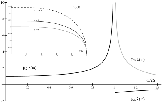
Figure 5.1: The response function $\lambda(\omega,T)$ as a function of frequency for $T=0$. The inset shows $\lambda(\omega,T)$ as a function of temperature at $\omega=\Delta(T)$.

At frequencies below the pair-breaking edge, $\omega<2\Delta$, $\lambda(\omega)$ is real and positive; the frequency and temperature dependence is shown in Fig. 5.1. Note that $\lambda(\omega)$ is nominally of order one, except near $T_{c}$ where $\lambda\sim(T_{c}-T)$, and for $\omega\rightarrow 2\Delta$ where $\lambda$ has a weak singularity, $\lambda\sim(2\Delta-\omega)^{-1/2}$. Above the pair-breaking edge $\lambda(\omega)$ has an imaginary part,

$$\mbox{Im}\,\lambda(\omega,T)=\frac{\pi}{2}\left(\frac{2\Delta}{\omega}\right)\,\frac{\tanh(\omega/4T)}{\sqrt{(\omega/2\Delta)^{2}-1}}\,,\quad\omega>2\Delta\,,$$ (5.103)

which determines (in part) the absorption of zero sound by pair breaking processes.

For a purely p-wave pairing interaction the equilibrium gap equation implies that $\gamma=2/V_{1}$. This relation is used to eliminate the pairing interaction $V_{1}$ and the cutoff-dependent integral $\gamma$ from the time-dependent gap equation that determines the order parameter collective modes. The solutions, Eqs. (5.97,5.98,5.99), are identical with those obtained by solving the linearized quasiclassical transport equations [59, 58].

The dispersion relations for the order parameter collective modes are found by substituting the solutions (5.98) and (5.99) into the nonequilibrium gap equation, Eq. (5.49). For a purely p-wave pairing interaction, ${\bm{d}}^{+}$ and ${\bm{d}}^{-}$ have the form,

$$d^{\pm}_{i}(\hat{\bm{p}},{\bm{q}};\omega)=D^{\pm}_{ij}({\bm{q}},\omega)\,\hat{\bm{p}}_{j}\,,$$ (5.104)

and satisfy the equations,

$$\int\frac{d\Omega_{\hat{\bm{p}}}}{4\pi}\,\lambda(\omega,\eta)\,\big{[}(\omega^{2}-\eta^{2}){\bm{d}}^{+}-4{\bm{\Delta}}({\bm{\Delta}}\cdot{\bm{d}}^{+})\big{]}_{i}\,\,\hat{\bm{p}}_{j} = 0\;,$$ (5.105)

$$\int\frac{d\Omega_{\hat{\bm{p}}}}{4\pi}\,\lambda(\omega,\eta)\,\big{[}(\omega^{2}-\eta^{2}-4\Delta^{2}){\bm{d}}^{-}+4{\bm{\Delta}}({\bm{\Delta}}\cdot{\bm{d}}^{-})$$

$$-2{\bm{\Delta}}\left(\omega\varepsilon^{+}+\eta\varepsilon^{-}\right)\big{]}_{i}\,\,\hat{\bm{p}}_{j} = 0\,.\hskip 28.45274pt$$ (5.106)

Since the equilibrium state is the pseudo-isotropic state give in Eq. (5.6), with $J=0$ and an isotropic gap, the correct basis functions describing the excitations of the condensate are the spherical tensors, $t^{J,M}_{ij}$,

$$D_{ij}^{\pm}=\sum^{2}_{J=0}\,\sum^{+J}_{M=-J}\,D_{J,M}^{\pm}\,t^{J,M}_{ij}\,,$$ (5.107)

where

$$t^{0,0}_{ij} = \frac{1}{\sqrt{3}}\,\delta_{ij}\;,$$

$$t^{1,M}_{ij} = \frac{1}{\sqrt{2}}\,\epsilon_{ijk}\,{\bm{u}}^{M}_{k}\,;\quad{\bm{u}}^{0}_{k}=\hat{\bm{z}}_{k}\,,\quad{\bm{u}}^{\pm 1}_{k}=-\frac{1}{\sqrt{2}}\,\left(\hat{\bm{x}}\pm i\hat{\bm{y}}\right)_{k}\,,$$ (5.108)

and

$$t_{ij}^{2,0} = \sqrt{\frac{3}{2}}\,\big{[}\hat{\bm{z}}_{i}\hat{\bm{z}}_{j}-{{1}\over{3}}\delta_{ij}\big{]}\,,$$

$$t_{ij}^{2,\pm 1} = \mp\frac{1}{\sqrt{2}}\,\left[(\hat{\bm{x}}\pm i\hat{\bm{y}})_{i}\,\hat{\bm{z}}_{j}+\hat{\bm{z}}_{i}(\hat{\bm{x}}\pm i\hat{\bm{y}})_{j}\right]\,,$$

$$t_{ij}^{2,\pm 2} = \mp\frac{1}{2}(\hat{\bm{x}}\pm i\hat{\bm{y}})_{i}(\hat{\bm{x}}\pm i\hat{\bm{y}})_{j}\,.$$ (5.109)

These spherical tensors satisfy the relations,

$$\left(t^{J,M}_{ij}\right)^{*}=t^{J,-M}_{ij}\,,$$ (5.110)

are orthogonal,

$$\sum_{ij}\,t^{J,M}_{ij}\,t_{ij}^{J^{\prime},M^{\prime*}}=\delta_{JJ^{\prime}}\,\delta_{MM^{\prime}}\,,$$ (5.111)

and are related to the spherical harmonic functions for the direction $\hat{\bm{a}}$ by

$${\cal Y}_{JM}(\hat{\bm{a}})=\left\{\begin{matrix}\sqrt{\frac{3}{4\pi}}\,t^{0,0}_{ij}\,\hat{\bm{a}}_{i}\hat{\bm{a}}_{j}\,;\quad J=0\,,\cr\sqrt{\frac{3}{8\pi}}\,\epsilon_{ilm}\,t_{lm}^{1,M}\,\hat{\bm{a}}_{i}\,;\quad J=1\,,\cr\sqrt{\frac{15}{8\pi}}\,t_{ij}^{2,M}\,\hat{\bm{a}}_{i}\hat{\bm{a}}_{j}\,;\quad J=2\,.\end{matrix}\right.$$ (5.112)

The quantization axis $\hat{\bm{z}}$ defining the orientation of the order parameter modes is determined by the propagation direction $\hat{\bm{q}}$ in the zero-field limit, as is clear from Eqs. (5.105) and (5.106) in which $\hat{\bm{q}}$ is the only direction entering the equations of motion for ${\bm{d}}^{\pm}$.

Here we are only concerned with the $J=2^{+},2^{-}$, and $0^{-}$ modes. Their dispersion relations are obtained by projecting the amplitudes $D^{\pm}_{JM}$ out of Eqs. (5.105) and (5.106). Note that the real (${\bm{d}}^{+}$) and imaginary (${\bm{d}}^{-}$) modes are decoupled from one another, a consequence of particle-hole symmetry which is built into the quasiclassical equations. In the limit $q\rightarrow 0$ the modes with different $(J,M)$ also decouple. In particular, the $J=2^{+}$ modes satisfy the homogenous equation,

$$\lambda(\omega)\left[\omega^{2}-\frac{8}{5}\Delta^{2}\right]\,D_{2,M}^{+}({\bm{q}}=0,\omega)=0\,,$$ (5.113)

for all $M=\{-2,...,2\}$. The five-fold degeneracy of the $J=2^{+}$ modes is a consequence of rotational invariance of the B-phase, while the homogeneity of Eqs. (5.105) and (5.113), in particular the absence of any coupling to the density or longitudinal current follows from particle-hole symmetry. The degeneracy is partially lifted for modes with non-zero pair momentum ${\bm{q}}$;

$$\omega_{M}^{2}=\frac{8}{5}\Delta^{2}+c_{M}^{2}q^{2}\,,$$ (5.114)

where the velocities $c_{M}$ are approximately given by $c_{\pm 2}^{2}\simeq\frac{1}{5}v_{f}^{2}$, $c_{\pm 1}^{2}\simeq\frac{2}{5}v_{f}^{2}$, and $c_{0}^{2}\simeq\frac{7}{15}v_{f}^{2}$ for $qv_{f}\ll\Delta$ [72]. The degeneracy of the $J=2^{+}$ modes is fully lifted by a magnetic field [69]. In the field-dominated regime, $\Delta>\gamma H\gg(qv_{f})^{2}/\Delta$, the modes exhibit a linear Zeeman splitting [62, 60],

$$\omega_{M}=\sqrt{8/5}\,\Delta+M\,g_{2^{+}}\,\omega_{L}\,,$$ (5.115)

where

$$g_{2^{\pm}}=\frac{1}{12}\left[1\pm\frac{\left(1-y(T)\right)}{\lambda(\omega_{2^{\pm}})}\right]\,,$$ (5.116)

is the Landé factor for the mode,

$$\omega_{L}=\frac{\gamma H}{1+{{1}\over{3}}F_{0}^{a}\left[2+y(T)\right]}\,,$$ (5.117)

is the effective Larmor frequency, and $y(T)$ is the Yosida function. The five-fold Zeeman splitting was observed by Avenel, et al. [6], and provided clear identification of the of the absorption peaks discovered by Giannetta et al. [24] and Mast et al. [43] as the $J=2^{+}$ modes.

In summary, if the Zeeman splitting in a small magnetic field ($\gamma H\ll\Delta$), and the effects of dispersion and damping due to quasiparticle collisions are taken into account, then the factor $(\omega^{2}-\frac{8}{5}\Delta^{2})$ in Eq. (5.113) is replaced by $(\omega^{2}+2i\omega\Gamma-\omega_{M}^{2}-c_{M}^{2}q^{2})$, where $1/\Gamma$ is the lifetime and $c_{M}$ determines the phase velocity of the $J=2^{+}$, $M$ mode. Complete expressions for the mode frequencies, Landé g-factors and mode velocities including Fermi-liquid and higher-order pairing effects are given in Refs. [59, 60, 22].

Although the $J=2^{+}$ mode is uncoupled to sound within the quasiclassical theory for the linear response, there is nevertheless a weak coupling of the $J=2^{+}$ modes to zero sound arising from the small, but nonvanishing particle-hole asymmetry of ³He. In particular, if we retain the weak energy dependence of the density of states, $N(\xi_{{\bm{p}}})\simeq N(0)+N^{\prime}(0)\xi_{{\bm{p}}}+\ldots$, then the right side of Eq. (5.113) is replaced by a term of the form,

$$\int\frac{d\Omega_{{\bm{p}}}}{4\pi}\,\zeta(\omega,\eta)\,\left[{\bm{\Delta}}(\omega\varepsilon^{+}+\eta\varepsilon^{-})\right]_{i}\,\hat{\bm{p}}_{j}$$ (5.118)

where $\zeta\sim N^{\prime}(0)T_{c}/N(0)\lambda\sim T_{c}/E_{f}$ is a measure of the particle-hole asymmetry of ³He [31].

We now derive dynamical equations describing the linear coupling of the $J=0^{-}$ and $J=2^{-}$ modes to density oscillations. These equations are later used in the derivation of the nonlinear constitutive equations, Eqs. (5.25) and (5.2). The $J=0^{-}$ mode describes oscillations in the phase of the equilibrium order parameter and is the Goldstone mode associated with broken gauge symmetry. If Eq. (5.106) is contracted with $t_{ij}^{0,0}$ the result is

$$\int\frac{d\Omega_{{\bm{p}}}}{4\pi}\lambda(\omega,\eta)\left[\Delta^{2}(\omega\varepsilon^{+}+\eta\varepsilon^{-})-{{1}\over{2}}(\omega^{2}-\eta^{2}){\bm{\Delta}}\cdot{\bm{d}}^{-}\right]=0\,,$$ (5.119)

which to first order in $1/s^{2}=(qv_{f}/\omega)^{2}\simeq(v_{f}/c_{1})^{2}\sim 1/F^{s}_{0}$ gives

$$\left(\omega^{2}-{{1}\over{3}}(qv_{f})^{2}\right)\,\frac{D^{-}_{0,0}}{\sqrt{3}}=2\Delta\left(\omega\varepsilon_{0}+{{1}\over{3}}qv_{f}\varepsilon_{1}\right)\,.$$ (5.120)

For $q=0$ and $\omega\ll\Delta$ Eq. (5.120) reduces to the Josephson equation, $i\partial_{t}\varphi=-2\varepsilon_{0}$, where $\varphi$ is the phase of the local equilibrium order parameter, ${\bm{\Delta}}(\hat{\bm{p}},t)={\bm{\Delta}}(\hat{\bm{p}})\,e^{i\varphi(t)}$ $\simeq{\bm{\Delta}}(\hat{\bm{p}})\left(1+i\varphi\right)$, in which case $D_{0,0}^{-}/\sqrt{3}=2\Delta\varphi$; and $\varepsilon_{0}$ is the scalar shift in the quasiparticle energy. For $q\neq 0$, Eq. (5.120) is identified as the Bogoliubov-Anderson mode in the limit $\omega\ll\Delta$.

Similarly, the contraction of Eq. (5.106) with $t_{ij}^{2,M^{*}}$ gives the dispersion relation for the $J=2^{-}$ modes. In the long-wavelength limit,

$$\frac{1}{6}\lambda(\omega)\left[\omega^{2}-\omega_{M}(q)^{2}\right]\,D_{2,M}^{-}(q,\omega)\negthickspace\negthickspace\negthickspace\negthickspace = \negthickspace\negthickspace\negthickspace\negthickspace\int\frac{d\Omega_{{\bm{p}}}}{4\pi}\,t_{ij}^{2,M^{*}}\,\hat{\bm{p}}_{i}\hat{\bm{p}}_{j}\,\lambda(\eta,\omega)\hskip 28.45274pt$$

$$\times \negthickspace\negthickspace\negthickspace\negthickspace\bigg{[}\Delta(\omega\varepsilon^{+}+\eta\varepsilon^{-})-{{1}\over{2}}\left(\omega^{2}-\eta^{2}\right)\,\frac{D^{-}_{0,0}}{\sqrt{3}}\bigg{]}\,,$$

where

$$\omega_{M}^{2}=\frac{12}{5}\Delta^{2}+c_{M}^{2}q^{2}\,,$$ (5.122)

are the $J=2^{-},M$ mode frequencies. The mode velocities are to a good approximation the same as those given above for the $J=2^{+}$ modes, and the right side determines the coupling of the $J=2^{-}$ modes to the density fluctuations. To leading order in $(qv_{f}/\omega)$ we can neglect the $q$-dependence of $\lambda(q,\omega)$. To further simplify matters we assume that $A^{s}_{l}=0$ for $l\geq 2$. Only the $l=0$ and $l=1$ projections of the mean fields, $\varepsilon_{0}$ and $\varepsilon_{1}$, which are proportional to the density and current fluctuations

$$\varepsilon_{0}={{1}\over{2}}A_{0}^{s}\,\delta g_{0}\,,\qquad\varepsilon_{1}={{1}\over{2}}A_{1}^{s}\,\delta g_{1}\,,$$ (5.123)

contribute to Eq. (5.4). These expressions are combined with the particle conservation law given in Eq. (5.9) to relate $\varepsilon_{1}$ to $\delta g_{0}$. Then to leading order in $1/s^{2}$ the phase mode and the density fluctuation are related by

$$\frac{D^{-}_{0,0}}{\sqrt{3}}\simeq\left(\frac{\Delta}{\omega}\right)\,\delta g_{0}(q,\omega)\,,$$ (5.124)

and, thus the equations of motion for the $J=2^{-}$ modes become,

$$\left(\omega^{2}-\omega_{M}(q)^{2}\right)\,D_{2,M}^{-}(q,\omega)=\frac{6}{5}\,G_{M}^{*}\,\frac{\Delta\,(c_{1}q)^{2}}{\omega(1+F_{0}^{s})}\,\delta g_{0}(q,\omega)\,,$$ (5.125)

where $G_{M}=\sqrt{\frac{2}{3}}\,\delta_{M,0}$. In zero field the density and current fluctuations excite only the $J=2^{-},M=0$ mode (with $\hat{\bm{q}}$ being the quantization axis for the excited pairs). However, in a magnetic field, $\Delta>\gamma H\gg(qv_{f})^{2}/\Delta$, the quantization axis is fixed by the magnetic field, $\hat{\bm{z}}=\underline{{\bm{R}}}(\hat{\bm{n}},\theta)\cdot\hat{\bm{H}}$, and the $J=2^{-}$ modes exhibit a Zeeman effect; $\omega_{M}=\sqrt{12/5}\,\Delta+M\,g_{2^{-}}\,\omega_{L}$. Equation (5.125) still holds, but with the coupling strengths given by

$$G_{M}=\sqrt{8\pi/15}\,{\cal Y}_{2M}(\hat{\bm{q}})\,.$$ (5.126)

For propagation parallel to the quantization axis only the $M=0$ mode is excited; however, for $\hat{\bm{q}}\neq\hat{\bm{z}}$, all five modes can couple to the density wave. The Zeeman splitting of the $J=2^{-}$ modes has recently been observed by Movshovich, et al. [47].

As discussed in Sec. (5.2), the phase velocity and attenuation of zero sound are determined by the longitudinal components of the stress tensor, $\delta\Pi\sim\delta g_{2}$. Taking $l=2$ moment of Eq. (5.97) gives

$$\delta g_{2}(q,\omega)=\frac{2}{5}\frac{\left(1-\lambda(\omega)\right)}{1+F_{0}^{s}}\left(\frac{c_{1}q}{\omega}\right)^{2}\delta g_{0}(q,\omega)+\frac{\omega\lambda(\omega)}{5\Delta}\sum_{M}G^{M}\,D_{2,M}^{-}(q,\omega)\,,$$ (5.127)

to leading order in $1/s^{2}$. Combining Eq. (5.127) with the wave equation, Eqs. (5.14) and (5.53), we obtain the dispersion relation for collisionless sound,

$$\omega^{2} = c_{1}^{2}q^{2}\big{[}1+2\xi(q,\omega)\big{]}\,,$$ (5.128)

$$\xi\equiv\frac{\delta\Pi}{\delta n} = \frac{2}{5}\left(\frac{c_{1}q}{\omega}\right)^{2}\left(\frac{1}{1+F^{s}_{0}}\right)$$

$$\times \left[\left(1-\lambda(\omega)\right)+\frac{3}{5}\lambda(\omega)\sum_{M}|G_{M}|^{2}\frac{\omega^{2}}{(\omega+i\Gamma)^{2}-\omega_{M}(q)^{2}}\right]\,.$$

The first term proportional to $(1-\lambda(\omega))$ gives a shift in the phase velocity for $\omega<2\Delta$ from non-condensate excitations. In the limit $\omega\rightarrow 0$, $T\rightarrow 0$ this shift vanishes, as does the shift in phase velocity due to the off-resonant excitation of the $J=2^{-}$ modes represented by the second set of terms in (5.4). At high frequencies, $\omega\sim\omega_{M}$, the $J=2^{-}$ modes contribute significantly to both the phase velocity and damping of sound,

$$\frac{\delta v(\omega)}{c_{1}}\bigg{|}_{2^{-}\,\mbox{\footnotesize modes}} = \mbox{Re}\,\xi_{2^{-}\,\mbox{\footnotesize modes}}\simeq\frac{6}{25}\,\frac{\lambda(\omega)}{1+F^{s}_{0}}\,\sum_{M}|G_{M}|^{2}\left(\frac{\omega^{2}}{\omega^{2}-\omega^{2}_{M}}\right)\,,$$ (5.130)

$$\alpha_{2^{-}\,\mbox{\footnotesize modes}} = -q\,\mbox{Im}\,\xi_{2^{-}\,\mbox{\footnotesize modes}}\simeq\frac{6\pi}{25}\,\frac{\omega}{c_{1}}\frac{\lambda(\omega)}{1+F^{s}_{0}}\,\sum_{M}|G_{M}|^{2}\delta(\omega^{2}-\omega^{2}_{M})\,.$$ (5.131)

In addition to the resonant absorption and anomalous dispersion of zero sound for $\omega\simeq\omega_{M}$, the $J=2^{-}$ modes also modify the pair-breaking threshold. For $\omega>2\Delta$ the pair-breaking attenuation arises from $\mbox{Im}\,\lambda\sim 1/\sqrt{\omega-2\Delta}$. However, the singularity at $\omega=2\Delta$ is suppressed by the off-resonant coupling to the $J=2^{-}$ mode, so that

$$\alpha_{\mbox{\footnotesize pair-breaking}}\simeq\frac{6}{25}\,\frac{\omega}{c_{1}}\,\frac{\mbox{Im}\,\lambda(\omega)}{1+F^{s}_{0}}\,\left(\frac{\omega^{2}-4\Delta^{2}}{\omega^{2}-\frac{12}{5}\Delta^{2}}\right)\sim\sqrt{\omega-2\Delta}\,,$$ (5.132)

in agreement with Wölfle [74] and Serene [63], and qualitative agreement with experimental measurements of the pair-breaking attenuation [24, 46, 16]. Finally, we remark that if we include the particle-hole asymmetry corrections, then the dispersion function $\xi(q,\omega)$ also includes resonant coupling to the $J=2^{+}$ modes of the form [31],

$$\xi_{2^{+}}=\frac{6}{25}\left(\frac{c_{1}q}{\omega}\right)^{2}\left(\frac{1}{1+F^{s}_{0}}\right)\,[\zeta(\omega)]^{2}\,\sum_{M}|G_{M}|^{2}\left(\frac{\omega^{2}}{(\omega+i\Gamma)^{2}-\omega_{2^{+}M}(q)^{2}}\right)\,,$$

$$\mbox{with}\,\zeta\sim\frac{T_{c}}{E_{f}}\,\lambda\,.$$ (5.133)

5.5 Nonlinear response

In Sec. (5.2) we argued that even without exact particle-hole symmetry a nonlinear coupling between the $J=2^{+}$ modes and zero sound exists, and is of the form

$$\delta g_{2}(\omega)=\sum_{M}\frac{1}{\Delta^{2}}\int d\nu\,\Xi^{(1)}_{M}(\omega,\nu,\omega-\nu)\,\delta g_{0}(\nu)\,D^{+}_{2,M}(\omega-\nu)\,,$$ (5.134)

$$\frac{\bar{\lambda}(\omega)}{6}\negthickspace\left[\omega^{2}-\omega_{M}^{2}\right]\negthickspace D^{+}_{2,M}(\omega)\negthickspace=\negthickspace\frac{1}{\Delta^{2}}\negthickspace\int\negthickspace d\nu\Xi^{(2)}_{M}\negthickspace(\omega,\negthickspace\nu,\negthickspace\omega\negthickspace-\negthickspace\nu)\delta g_{0}(\nu)\delta g_{0}(\omega\negthickspace-\negthickspace\nu)\,.$$ (5.135)

The wave vector dependence of the nonlinear terms is suppressed for clarity. In fact the constitutive equations can be written in the forms given in (5.25) and (5.2), as the kernels $\Xi^{\left({1}\right)}_{M}\left({\omega,\nu,\omega-\nu}\right)$ and $\Xi^{\left({2}\right)}_{M}\left({\omega,\nu,\omega-\nu}\right)$ are determined by the same coupling function,

$$A_{M}({\bm{q}},\omega;{\bm{s}},\nu;{\bm{q}}-{\bm{s}},\omega-\nu)=\frac{1}{5}\left(\frac{c_{1}s}{\nu}\right)^{2}\,Z_{M}(\hat{\bm{q}},\hat{\bm{s}})\,\tilde{A}(\omega,\nu,\omega-\nu)\,,$$ (5.136)

where the frequency and temperature dependence of the coupling strength is contained in the factor $\tilde{A}(\omega,\nu,\omega-\nu)$, which can be written as a linear combination of Tsuneto functions, $\lambda(x)$, evaluated at the frequencies $x=\{\omega,\nu,\omega-\nu\}$ with coefficients that are algebraic functions of $\omega$, $\nu$, and $\omega-\nu$ and the energy gap $\Delta(T)$. The dependence of $A_{M}$ on $\hat{\bm{q}}$ and $\hat{\bm{s}}$, the propagation directions of the two sound waves, and the magnetic quantum $M$ is contained in the factor

$$Z_{M}(\hat{\bm{q}},\hat{\bm{s}})=(\hat{\bm{q}}\cdot\hat{\bm{s}})\,\hat{\bm{s}}_{i}\,t^{2,M}_{ij}\hat{\bm{q}}_{j}-{{1}\over{3}}\,\hat{\bm{q}}_{i}\,t^{2,M}_{ij}\,\hat{\bm{q}}_{j}-{{1}\over{3}}\,\hat{\bm{s}}_{i}\,t^{2,M}_{ij}\,\hat{\bm{s}}_{j}\,.$$ (5.137)

The explicit expression for $\tilde{A}$ is derived below.

The right sides of Eqs. (5.134) and (5.135) come from contributions to the quasiclassical propagator which are second order in the nonequilibrium mean fields, and are derived from Eq. (5.69). The explicit calculation of $\delta\hat{g}^{(2)}$ is lengthy, particularly at finite wavevector; however, gauge and Galilean invariance and the generalization of the Onsager-type relations, Eqs. (5.78) and (5.79), for the nonlinear response, reduce the number of independent terms. Furthermore, it is necessary to calculate $\Xi^{(1)}$ and $\Xi^{(2)}$ only to leading order in $1/s^{2}$ since the kernels of Eqs. (5.134) and (5.135) need only be evaluated at $q=0$.

Since we are interested here in weak nonlinearities arising from the coupling of sound to the $J=2^{+}$ modes, the density and current induce oscillations of the same frequency in the mean fields, $\varepsilon^{+}$ and $\varepsilon^{-}$, in the phase of the order parameter (the $J=0^{-}$ mode), and the (off-resonant) $J=2^{-}$ mode. To derive Eqs. (5.134) and (5.135) it is simplest to eliminate the phase of the order parameter by a gauge transformation. We then write the nonequilibrium self energy in the form

$$\delta\hat{\sigma}=\varepsilon^{+}\hat{1}+\varepsilon^{-}\hat{\tau}_{3}+{\bm{d}}^{-}\cdot\hat{\tau}_{3}\,\hat{{\bm{\delta}}}+{\bm{d}}^{+}\cdot\hat{{\bm{\delta}}}\,,$$ (5.138)

where $\varepsilon^{+}$ and $\varepsilon^{-}$ are related to the density oscillation by $\varepsilon^{+}={{1}\over{2}}A^{s}_{0}\,\delta g_{0}$ and $\varepsilon^{-}={{1}\over{2}}A^{s}_{1}\,\omega\,\left(\hat{\bm{p}}\cdot\hat{\bm{q}}\right)$ $\delta g_{0}/(1+F^{s}_{0})$. The oscillations in the imaginary part of the order parameter, ${\bm{d}}^{-}$, contain only a contribution from the off-resonant excitation of the $J=2^{-}$ mode (from Eq. (5.125)), and is related to the density oscillation by

$${\bm{d}}^{-}({\bm{q}},\omega)=\frac{\mu(\omega)}{1+F_{0}^{s}}\,\left(\frac{c_{1}q}{\omega}\right)^{2}{\bm{R}}(\hat{\bm{q}})\,\delta g_{0}(q,\omega)\,,$$ (5.139)

where $\mu(\omega)={{6}\over{5}}\omega\Delta/\left(\omega^{2}-{{12}\over{5}}\Delta^{2}\right)$ and ${\bm{R}}(\hat{\bm{q}})=\hat{\bm{q}}(\hat{\bm{p}}\cdot\hat{\bm{q}})-{{1}\over{3}}\hat{\bm{p}}$.

These linear relations are used below to obtain the response of ³He-B arising from the nonlinear coupling of sound to the $J=2^{+}$ modes. To obtain these nonlinear couplings we expand the $4\times 4$ matrix propagator $\delta\check{g}$ and the self energy $\delta\hat{\sigma}$ in terms of the matrices $\{\hat{\gamma}_{a}\}$ as in Eq. (5.46), then the expansion coefficients for the second-order contribution to the propagator obtained from Eq. (5.69) are given by

$$\delta g_{a}({\bm{q}},\omega) = \sum_{b,c=1}^{16}\int\frac{d\nu}{2\pi}\int\frac{d^{3}s}{(2\pi)^{3}}\,$$

$$\times e_{a}\,X_{abc}(\omega,\nu,\omega-\nu)\,\delta\sigma_{b}({\bm{s}},\nu)\,\delta\sigma_{c}({\bm{q}}-{\bm{s}},\omega-\nu)\,,$$

where

$$X_{abc}(\omega,\nu,\omega-\nu) = \bar{X}_{abc}(\omega,\nu,\omega-\nu)+\bar{X}_{acb}(\omega,\nu,\omega-\nu)\,,$$

$$\bar{X}_{abc}(\omega,\nu,\omega-\nu) = \mu^{RRK}_{abc}+\mu^{RKA}_{abc}+\mu^{KAA}_{abc}\,,$$ (5.141)

and $\mu^{QST}_{abc}$ involves a product of the three equilibrium propagators $\hat{G}^{Q}$, $\hat{G}^{S}$ and $\hat{G}^{T}$ [$Q,S,T=\{R,K,A\}$],

$$\mu^{QST}_{abc}(\omega,\nu,\omega-\nu)=\int\frac{d\epsilon}{2\pi i}\int d\xi_{{\bm{p}}}\,\mbox{Tr}\bigg{[} \hat{\gamma}_{a} \hat{G}_{0}^{Q}(\xi_{{\bm{p}}}+{{1}\over{2}}\eta,\epsilon+{{1}\over{2}}\omega)$$ (5.142)

$$\hat{\gamma}_{b} \hat{G}_{0}^{S}(\xi_{{\bm{p}}}-{{1}\over{2}}\eta+\eta^{\prime},\epsilon-{{1}\over{2}}\omega+\nu)$$

$$\hat{\gamma}_{c} \hat{G}_{0}^{T}(\xi_{{\bm{p}}}-{{1}\over{2}}\eta,\epsilon-{{1}\over{2}}\omega)\bigg{]}\,,$$

with $\eta=v_{f}\,\hat{\bm{p}}\cdot{\bm{q}}$ and $\eta^{\prime}=v_{f}\,\hat{\bm{p}}\cdot{\bm{s}}$. The expression for $X_{abc}$ contains six terms corresponding to the possible time orderings of the propagators. It follows from its definition that

$$X_{abc}(\omega,\nu,\omega-\nu)=X_{acb}(\omega,\omega-\nu,\nu)\,.$$ (5.143)

In addition the identities $\mbox{Tr}[\hat{A}\hat{B}]=\mbox{Tr}[\hat{B}\hat{A}]$ and $h^{R}=h^{A^{*}}$ imply

$$\mbox{Re}\,X_{abc}(\omega,\nu,\omega-\nu) = \mbox{Re}\,X_{bac}(-\nu,-\omega,\omega-\nu)$$ (5.144)

$$= \mbox{Re}\,X_{cba}(-\omega+\nu,\nu-\omega)\,,$$

which are the nonlinear generalizations of the Onsager-like relations given in (5.78). As is the case for the linear response functions further relations follow from gauge, Galilean and rotational invariance. It is straight forward to show that Galilean invariance implies

$$\nu\,X_{a2b}(\omega,\nu,\omega-\nu)=\eta^{\prime}\,X_{a1b}(\omega,\nu,\omega-\nu)\,,$$ (5.145)

$$(\omega-\nu)\,X_{a2b}(\omega,\nu,\omega-\nu)=(\eta-\eta^{\prime})\,X_{a1b}(\omega,\nu,\omega-\nu)\,,$$ (5.146)

and thus, the mean fields, $\varepsilon^{+}$ and $\varepsilon^{-}$, appear only in the combinations $\nu\varepsilon^{+}({\bm{s}},\nu)+\eta^{\prime}\varepsilon^{-}({\bm{s}},\nu)$ and $(\omega-\nu)\varepsilon^{+}({\bm{q}}-{\bm{s}},\omega-\nu)+(\eta-\eta^{\prime})\varepsilon^{-}({\bm{q}}-{\bm{s}},\omega-\nu)$. Consequently, it is convenient to introduce the quantity

$$\omega\theta({\bm{q}},\omega)\equiv\omega\,\varepsilon^{+}({\bm{q}},\omega)+\eta\,\varepsilon^{-}({\bm{q}},\omega)\,.$$ (5.147)

We now write down the general form for the distribution function and pair amplitudes, $\delta g^{+}$, $\delta{\bm{f}}^{+}$ and $\delta{\bm{f}}^{-}$, which are second order in the non-equilibrium mean fields. Particle-hole symmetry and the relations (5.145) and (5.146) imply that there are only three independent coupling tensors $X_{11j}$,$X_{1lj}$ and $X_{lmj}$ (where $j=10,11,12$ and $l,m=14,15,16$) which appear in the expressions for $\delta g^{+}$, $\delta{\bm{f}}^{-}$ and $\delta{\bm{f}}^{+}$. Gauge and rotational invariance further imply that these coupling tensors can be written in the form

$$X_{11j} = A\,\Delta_{j}X_{1lj}=B\,\Delta_{l}\Delta_{j}+C\,\delta_{lj}$$

$$X_{lmj} = E\,\Delta_{l}\delta_{mj}+F\,\Delta_{m}\delta_{jl}+G\,\Delta_{j}\delta_{lm}+H\,\Delta_{l}\Delta_{j}\Delta_{m}\,.$$ (5.148)

The identity $X_{lmj}(\omega,\nu,\omega-\nu)=X_{mlj}(-\nu,-\omega,\omega-\nu)$ further implies

$$E(\omega,\nu,\omega-\nu)=-F(-\nu,-\omega,\omega-\nu)\,.$$ (5.149)

The second-order terms in $\delta g^{+}$, $\delta{\bm{f}}^{-}$ and $\delta{\bm{f}}^{+}$ are then given in terms of these seven coefficients,

$$\delta g^{+(2)}(\omega)=\int d\nu\,\Big{[} A(\omega,\nu,\omega-\nu)\,\theta(\nu){\bm{\Delta}}\cdot{\bm{d}}^{+}(\omega-\nu)$$ (5.150)

$$+ B(\omega,\nu,\omega-\nu)\,{\bm{\Delta}}\cdot{\bm{d}}^{-}(\nu)\,{\bm{\Delta}}\cdot{\bm{d}}^{+}(\omega-\nu)$$

$$+ C(\omega,\nu,\omega-\nu)\,{\bm{d}}^{-}(\nu)\cdot{\bm{d}}^{+}(\omega-\nu)\Big{]}\,,$$

$$\delta{\bm{f}}^{-(2)}(\omega)=\int d\nu\Big{[} B(-\nu,-\omega,\omega-\nu)\,\theta(\nu)\,{\bm{\Delta}}\cdot{\bm{d}}^{+}(\omega-\nu)\,{\bm{\Delta}}$$ (5.151)

$$+ C(-\nu,-\omega,\omega-\nu)\,\theta(\nu)\,{\bm{d}}^{+}(\omega-\nu)$$

$$+ E(\omega,\nu,\omega-\nu)\,{\bm{d}}^{-}(\nu)\cdot{\bm{d}}^{+}(\omega-\nu)\,{\bm{\Delta}}$$

$$+ F(\omega,\nu,\omega-\nu){\bm{\Delta}}\cdot{\bm{d}}^{-}(\nu)\,{\bm{d}}^{+}(\omega-\nu)$$

$$+ G(\omega,\nu,\omega-\nu)\,{\bm{\Delta}}\cdot{\bm{d}}^{+}(\omega-\nu)\,{\bm{d}}^{-}(\nu)$$

$$+ H(\omega,\nu,\omega-\nu)\,{\bm{\Delta}}\cdot{\bm{d}}^{-}(\nu)\,{\bm{\Delta}}\cdot{\bm{d}}^{+}(\omega-\nu)\,{\bm{\Delta}}\Big{]}\,,$$

$$\delta{\bm{f}}^{+(2)}(\omega)=\int d\nu\Big{[} A(\nu-\omega,\nu,-\omega)\,\theta(\nu)\,\theta(\omega-\nu)\,{\bm{\Delta}}$$

$$+ B(\nu-\omega,\nu,-\omega)\,{\bm{\Delta}}\cdot{\bm{d}}^{-}(\nu)\theta(\omega-\nu)\,{\bm{\Delta}}$$

$$+ B(-\nu,\omega-\nu,-\omega)\,\theta(\nu)\,{\bm{\Delta}}\cdot{\bm{d}}^{-}(\omega-\nu)\,{\bm{\Delta}}$$

$$+ C(\nu-\omega,\nu,-\omega)\theta(\omega-\nu)\,{\bm{d}}^{-}(\nu)$$

$$+ C(-\nu,\omega-\nu,-\omega)\,\theta(\nu)\,{\bm{d}}^{-}\left({\omega-\nu}\right)$$

$$+ E(\nu-\omega,\nu,-\omega)\,{\bm{\Delta}}\cdot{\bm{d}}^{-}(\omega-\nu)\,{\bm{d}}^{-}(\nu)$$

$$+ F(\nu-\omega,\nu,-\omega)\,{\bm{\Delta}}\cdot{\bm{d}}^{-}(\nu)\,{\bm{d}}^{-}(\omega-\nu)$$

$$+ G(\nu-\omega,\nu,-\omega)\,{\bm{d}}^{-}(\nu)\cdot{\bm{d}}^{-}(\omega-\nu)\,{\bm{\Delta}}$$

$$+ H(\nu-\omega,\nu,-\omega)\,{\bm{\Delta}}\cdot{\bm{d}}^{-}(\nu)\,{\bm{\Delta}}\cdot{\bm{d}}^{-}(\omega-\nu)\,{\bm{\Delta}}\Big{]}\,.$$

We have used Eqs. (5.5) and (5.142) for $X_{abc}(\omega,\nu,\omega-\nu)$ to calculate the seven coupling functions $A,B,C,E,F,G$ and $H$ for $q=0$. Each of these functions can be written in terms of the Tsuneto function, $\lambda(\omega)$,

$$A(\omega,\nu,\omega-\nu) = -4\Delta^{2}\,k_{1}(\omega,\nu,\omega-\nu)+(\omega-\nu)\,k_{2}(\omega,\nu,\omega-\nu)$$

$$B(\omega,\nu,\omega-\nu) = 2\omega\,k_{1}(\omega,\nu,\omega-\nu)$$

$$C(\omega,\nu,\omega-\nu) = \frac{-1}{\omega\Delta}\,\left[\nu^{2}\bar{\lambda}(\nu)-(\omega-\nu)^{2}\bar{\lambda}(\omega-\nu)\right]$$

$$\hskip 11.38109pt- 2(\omega-\nu)\Delta^{2}\,k_{1}(\omega,\nu,\omega-\nu)$$

$$E(\omega,\nu,\omega-\nu) = \frac{-2}{\nu\Delta}\left[\omega\bar{\lambda}(\omega)-(\omega-\nu)\bar{\lambda}(\omega-\nu)\right]$$

$$F(\omega,\nu,\omega-\nu) = \frac{-2}{\omega\Delta}\left[\nu\bar{\lambda}(\nu)+(\omega-\nu)\bar{\lambda}(\omega-\nu)\right]$$

$$G(\omega,\nu,\omega-\nu) = -4\Delta^{2}\,k_{1}(\omega,\nu,\omega-\nu)+k_{3}(\omega,\nu,\omega-\nu)$$

$$H(\omega,\nu,\omega-\nu) = 4\,k_{1}(\omega,\nu,\omega-\nu)\,,$$ (5.153)

where

$$k_{n}(\omega,\nu,\omega-\nu)\Delta = k_{n}(-\nu,-\omega,\omega-\nu)\,\Delta=\frac{2}{\omega\nu(\omega-\nu)}$$ (5.154)

$$\times \left[\omega^{n}\bar{\lambda}(\omega)+(-\nu)^{n}\,\bar{\lambda}(\nu)-(\omega-\nu)^{n}\,\bar{\lambda}(\omega-\nu)\right]\,.$$

The detailed derivation of these functions can be found in Ref. [44].

From the nonlinear propagators given in Eqs. (5.150), (5.151), and (5.5) we obtain the constitutive relations given in Eqs. (5.134) and (5.135). The nonlinear contribution to the longitudinal stress tensor is given in part by the $l=2$ projection of Eq. (5.150),

$$\int\frac{d\Omega_{{\bm{p}}}}{4\pi}\,P_{2}(\hat{\bm{p}}\cdot\hat{\bm{q}})\delta g^{+(2)}(\omega)=$$

$$\sum_{M}\,Z_{M}(\hat{\bm{q}},\hat{\bm{s}})\int d\nu\,L(\omega,\nu,\omega-\nu)\,\delta g_{0}(\nu)\,D^{+}_{2,M}(\omega-\nu)\,,$$ (5.155)

where

$$L(\omega,\nu,\omega-\nu)={{6}\over{35(1+F_{0}^{s})}}\,\left(\frac{c_{1}s}{\nu}\right)^{2}\Bigg{[}\Delta\,A+\mu(\nu)\big{(}{{2}\over{3}}\,B\,\Delta^{2}+{{7}\over{6}}\,C\big{)}\Bigg{]}\,,$$ (5.156)

and $Z_{M}$ is given by Eq. (5.137). There is also a contribution to the stress tensor from the $J=2^{-}$, $M=0$ mode [see Eq. (5.127)] which, as a result of the nonlinear term in Eq. (5.151), couples to the $J=2^{+}$ modes. This coupling is given by

$${{1}\over{6}}\bar{\lambda}(\omega)\left(\omega^{2}-{{12}\over{5}}\Delta^{2}\right)\,D^{-}_{2,0}(\omega) = -\sqrt{{{3}\over{2}}}\int\frac{d\Omega_{{\bm{p}}}}{4\pi}\,{\bm{R}}(\hat{\bm{q}})\cdot\delta{\bm{f}}^{-(2)}(\omega)$$

$$= -{{1}\over{5}}\,{{\sqrt{3/2}}\over{(1+F_{0}^{s})}}\sum_{M}\,Z_{M}(\hat{\bm{q}},\hat{\bm{s}})$$

$$\times \int d\nu\,\left(\frac{c_{1}s}{\nu}\right)^{2}\,K(\omega,\nu,\omega-\nu)\delta g_{0}(\nu)D^{+}_{2,M}(\omega-\nu)\,,$$

where

$$K(\omega,\nu,\omega-\nu) = \bigg{[}\frac{4}{7}\Delta^{2}B+C\big{]}(-\nu,-\omega,\omega-\nu)$$ (5.158)

$$+ {{2}\over{3}}\mu(\nu)\;\big{[}E+F+G+{{4}\over{7}}\Delta^{2}H\bigg{]}(\omega,\nu,\omega-\nu)\,.$$

In deriving (5.5) and (5.5) we made use of the identities

$${{1}\over{5}}Z_{M}(\hat{\bm{q}},\hat{\bm{s}}) = \int\frac{d\Omega_{{\bm{p}}}}{4\pi}\,P_{2}(\hat{\bm{p}}\cdot\hat{\bm{q}})\,\hat{\bm{p}}_{i}\,t_{ij}^{2,M}\,R_{j}(\hat{\bm{s}})$$ (5.159)

$$= \int\frac{d\Omega_{{\bm{p}}}}{4\pi}\,P_{2}(\hat{\bm{p}}\cdot\hat{\bm{s}})\,\hat{\bm{p}}_{i}\,t_{ij}^{2,M}\,R_{j}(\hat{\bm{q}})$$

$$= {{3}\over{2}}\int\frac{d\Omega_{{\bm{p}}}}{4\pi}\,{\bm{R}}(\hat{\bm{q}})\cdot{\bm{R}}(\hat{\bm{s}})\,\hat{\bm{p}}_{i}\,t_{ij}^{2,M}\,\hat{\bm{p}}_{j}$$

$$= {{7}\over{6}}\int\frac{d\Omega_{{\bm{p}}}}{4\pi}\,P_{2}(\hat{\bm{p}}\cdot\hat{\bm{q}})\,P_{2}(\hat{\bm{p}}\cdot\hat{\bm{s}})\,\hat{\bm{p}}_{i}\,t_{ij}^{2,M}\,\hat{\bm{p}}_{j}\,.$$

The resulting nonlinear stress is

$$\delta g_{2}(\omega)={{1}\over{5}}\omega\bar{\lambda}(\omega)\Delta\,\sqrt{{{3}\over{2}}}\,D^{-}_{2,0}(\omega)+\int\frac{d\Omega_{{\bm{p}}}}{4\pi}\,P_{2}(\hat{\bm{q}}\cdot\hat{\bm{s}})\,\delta g^{+(2)}(\omega)\,,$$ (5.160)

which upon combining Eqs. (5.5), (5.5) and (5.160) gives Eq. (5.134) with

$$\Xi_{M}^{(1)}(\omega,\nu,\omega-\nu)=\frac{1}{5(1+F_{0}^{s})}\left(\frac{c_{1}s}{\nu}\right)^{2}\,Z_{M}(\hat{\bm{q}},\hat{\bm{s}})\,\tilde{A}(\omega,\nu,\omega-\nu)\,,$$ (5.161)

where

$$\tilde{A}(\omega,\nu,\omega-\nu) = {{6}\over{7}}\Delta^{3}\,A(\omega,\nu,\omega-\nu)$$

$$+ {{4}\over{7}}\Delta^{4}\,\big{[}\mu(\nu)\,B(\omega,\nu,\omega-\nu)-\mu(\omega)\,B(-\nu,-\omega,\omega-\nu)\big{]}$$

$$+ \Delta^{2}\,\big{[}\mu(\nu)\,C(\omega,\nu,\omega-\nu)-\mu(\omega)\,C(-\nu,-\omega,\omega-\nu)\big{]}$$

$$- \frac{\mbox{\small 2}}{\mbox{\small 3}}\Delta^{3}\,\mu(\omega)\mu(\nu)\big{[}E+F+G+{{4}\over{7}}{H}\,\Delta^{2}\big{]}(\omega,\nu,\omega-\nu)\,.$$

Thus, the constitutive equation can be written as (5.25),

$$\delta\Pi(\omega)=\frac{1}{(1+F^{s}_{0})\Delta^{2}}\sum_{M}\int d\nu\,A_{M}(\omega,\nu,\omega-\nu)\,\delta n(\nu)\,D^{+}_{2,M}(\omega-\nu)\,,$$ (5.163)

with $A_{M}$ given by Eqs. (5.136) and (5.5). It follows directly from Eqs. (5.5) and (5.5) that the coupling function $A_{M}$ satisfies

$$A_{M}(\omega,\nu,\omega-\nu)=A_{M}(-\nu,-\omega,\omega-\nu)\,.$$ (5.164)

In a similar way the coupling functions $\Xi^{(2)}_{M}$ in Eq. (5.135) are found by substituting Eq. (5.5) into

$${{1}\over{6}}\bar{\lambda}(\omega)\left(\omega^{2}+2i\omega\Gamma-\omega_{M}^{2}-c_{M}^{2}q^{2}\right)D^{+}_{2,M}=-\int\frac{d\Omega_{{\bm{p}}}}{4\pi}t_{ij}^{2,M^{*}}\,\hat{\bm{p}}_{i}\delta{\bm{f}}_{j}^{+(2)}(\omega)\,.$$ (5.165)

Then to leading order in $1/s^{2}$

$$\Xi^{(2)}_{M}(\omega,\nu,\omega-\nu)=\frac{1}{1+F^{s}_{0}}\left|\frac{c_{1}({\bm{q}}-{\bm{s}})}{\omega-\nu}\right|^{2}\,A_{M}(\nu,-\omega,\nu-\omega)^{*}\,,$$ (5.166)

so that the second constitutive equation becomes,

$$\lambda(\omega)\,\left[\omega^{2}+2i\omega\Gamma-\omega_{2^{+},M}(q)^{2}\right]D^{+}_{2,M}$$ (5.167)

$$=\frac{6}{N(E_{f})^{2}}\int d\nu\,\left|\frac{c_{1}({\bm{q}}-{\bm{s}})}{\omega-\nu}\right|^{2}\,A_{M}(\nu-\omega,\nu,-\omega)^{*}\,\delta n(\nu)\,\delta n(\omega-\nu)\,.$$

Equations (5.163) and (5.167), together with the wave equation, Eq. (5.14), describe the weak nonlinear interaction of the $J=2^{+}$ modes with the density fluctuations of zero sound.

Before we discuss the consequences of these nonlinear constitutive equations we give a physical explanation of why the same coupling function $A_{M}$ appears in both Eqs. (5.163) and (5.167), and also satisfies the identity given in Eq. (5.164). Consider three wave packets with carrier frequencies ($\omega_{1}$, $\omega_{2}$, $\omega_{3}$) all propagating along the $z$-axis. The density and order parameter fluctuations can be written

$$\delta{n}(z,t) = N_{1}(z,t)\,e^{i(\omega_{1}t-q_{1}z)}+N_{2}(z,t)\,e^{i(\omega_{2}t-q_{2}z)}+\mbox{c.c.}\,,$$

$$D_{2,M}^{+}(z,t) = E_{M}(z,t)\,e^{i(\omega_{3}t-q_{3}z)}+\mbox{c.c.}\,.$$ (5.168)

We assume that the sound pulses are sufficiently short that the quasiparticle damping can be neglected (i.e. $\frac{1}{N_{j}}\,\mbox{$\displaystyle\frac{\partial N_{j}}{\partial t}$}\gg\Gamma\,,j=1,2$), that only one of the five $J=2^{+}$ modes is excited by the two sound waves, and that the three-wave resonance conditions for this mode hold: $\omega_{M}=\omega_{3}=\omega_{1}+\omega_{2}$, ${\bm{q}}_{3}={\bm{q}}_{1}+{\bm{q}}_{2}$. Substituting Eq. (5.5) into Eqs. (5.163), (5.167), and (5.14); and making a slowly varying envelope approximation, in which the amplitudes $N_{1}$, $N_{2}$ and $E_{M}$ are assumed to vary on time and length scales that are large compared to $1/\omega_{j}\sim 1/\Delta$ and $1/q_{j}\sim c_{1}/\Delta$, we obtain the following equations

$$i\left(\mbox{$\displaystyle\frac{\partial}{\partial t}$}-v_{1}\mbox{$\displaystyle\frac{\partial}{\partial z}$}\right)\,N_{1}=\frac{\omega_{1}A_{M}(\omega_{1},-\omega_{2},\omega_{3})}{\Delta(1+F_{0}^{s})}\,E_{M}\,N_{2}^{*}\,,$$

$$i\left(\mbox{$\displaystyle\frac{\partial}{\partial t}$}-v_{2}\mbox{$\displaystyle\frac{\partial}{\partial z}$}\right)\,N_{2}=\frac{\omega_{2}A_{M}(\omega_{2},-\omega_{1},\omega_{3})}{\Delta(1+F_{0}^{s})}\,E_{M}\,N_{1}^{*}\,,$$

$$\frac{i}{6}\bar{\lambda}(\omega_{3})\left(\mbox{$\displaystyle\frac{\partial}{\partial t}$}-v_{M}\mbox{$\displaystyle\frac{\partial}{\partial z}$}\right)\,E_{M}=\frac{A_{M}(-\omega_{1},-\omega_{2},-\omega_{3})^{*}}{2\Delta\omega_{3}N(E_{f})^{2}}\,N_{1}\,N_{2}\,,$$ (5.169)

where $v_{1}$ $v_{2}$ and $v_{M}$ are the group velocities of the sound waves and collective mode, respectively.

In a three-wave resonance the total number of quanta should be conserved, i.e. for each phonon of frequency $\omega_{1}$ that is destroyed a second phonon of frequency $\omega_{2}$ is also destroyed and a real squashon is created. Thus, we expect a continuity equation of the form

$$\left(\mbox{$\displaystyle\frac{\partial}{\partial t}$}-v_{1}\mbox{$\displaystyle\frac{\partial}{\partial z}$}\right)\frac{U_{1}}{\omega_{1}}=\left(\mbox{$\displaystyle\frac{\partial}{\partial t}$}-v_{2}\mbox{$\displaystyle\frac{\partial}{\partial z}$}\right)\frac{U_{2}}{\omega_{2}}=-\left(\mbox{$\displaystyle\frac{\partial}{\partial t}$}-v_{M}\mbox{$\displaystyle\frac{\partial}{\partial z}$}\right)\frac{U_{M}}{\omega_{3}}\,,$$ (5.170)

to hold, where $U_{j}/\omega_{j}$ is the number density of quanta of the mode with frequency $\omega_{j}$. It is straight forward to show (see e.g. Ref. [9]) that the energy density of zero-sound phonons is

$$U_{j}=\frac{N(E_{f})|N_{j}|^{2}}{1+F_{0}^{s}}\,,$$ (5.171)

while that of the real squashons is

$$U_{M}=\frac{\mbox{\small 2}}{\mbox{\small 3}}N(E_{f})\bar{\lambda}(\omega_{M})\,\omega_{M}^{2}\,|D^{+}_{M}|^{2}\,.$$ (5.172)

The conservation equations for the quanta follow directly from the three equations for the mode amplitudes and the identity given in (5.164). Equations (5.170) also occur in nonlinear optics [68] where they are called the Manley-Rowe relations after similar equations derived for nonlinear microwave circuits [41].

5.6 Stimulated Raman scattering and two-phonon absorption by the J=2⁺ modes

We now consider the three-wave resonance equations for two density waves interacting with the $J=2^{+}$ modes in more detail. The dynamics of the three-wave resonance is described by the wave equation, Eq. (5.14), which each of the two sound waves satisfies, with the constitutive equations given by Eq. (5.163) and the equation of motion for the the $J=2^{+}$ order parameter modes, Eq. (5.167). The density fluctuation resulting from two sound waves is

$$\delta{n}({\bm{x}},t)=\tilde{N}_{1}({\bm{x}},t)+\tilde{N}_{2}({\bm{x}},t)+\mbox{c.c.}\,,$$ (5.173)

$$\tilde{N}_{j}({\bm{x}},t)=N_{j}({\bm{x}},t)\,e^{i(\omega_{j}t-{\bm{q}}_{j}\cdot{\bm{x}})}\,;\quad j=1,2\,.$$ (5.174)

If the wave amplitudes vary slowly on the time scale of the collective mode lifetime, $1/\Gamma$, then Eq. (5.167) can be solved for $D_{2,M}^{+}({\bm{x}},t)$. The collective mode amplitude then contains terms oscillating with frequencies $\omega_{1}+\omega_{2}$, $\omega_{1}-\omega_{2}$, $2\omega_{1}$, $2\omega_{2}$ and $\omega=0$. One of these terms will dominate if its frequency $\omega_{a}$ and wavevector ${\bm{q}}_{a}$ satisfy the resonance condition,

$$\omega_{a}^{2}=\omega_{M}^{2}+c^{2}_{M}\,q_{a}^{2}\,.$$ (5.175)

First consider the case where the sum or difference of the frequencies of the two sound waves is approximately equal to one of the collective mode frequencies. The collective mode amplitudes are then given by

$$D_{2,M}^{+}({\bm{x}},t)=\frac{A_{M}(\omega_{1},-\omega_{2},\omega_{1}+\omega_{2})^{*}\,\tilde{N}_{1}({\bm{x}},t)\,\tilde{N}_{2}({\bm{x}},t)}{N(E_{f})^{2}\,\Delta\,\,\phi^{M}({\bm{q}}_{1}+{\bm{q}}_{2},\omega_{1}+\omega_{2})}+\mbox{c.c.}\,,$$ (5.176)

for $\omega_{1}+\omega_{2}\simeq\omega_{M}$, or

$$D_{2,M}^{+}({\bm{x}},t)=\frac{A_{M}(\omega_{1},\omega_{2},\omega_{1}-\omega_{2})^{*}\,\tilde{N}_{1}({\bm{x}},t)\,\tilde{N}_{2}({\bm{x}},t)}{N(E_{f})^{2}\,\Delta\,\,\phi^{M}({\bm{q}}_{1}-{\bm{q}}_{2},\omega_{1}-\omega_{2})}+\mbox{c.c.}\,,$$ (5.177)

if $\omega_{1}-\omega_{2}\simeq\omega_{M}$. The denominator is defined by

$$\phi^{M}(q,\omega)={{1}\over{6}}\bar{\lambda}(\omega)\left[\omega^{2}+2i\Gamma\omega-\omega_{M}^{2}-c_{M}^{2}q^{2}\right]\,.$$ (5.178)

If these solutions for the collective mode amplitudes and the density fluctuation given in Eq. (5.173) are substituted into the expression (5.163) for the stress, then the latter contains terms oscillating with frequency $\omega_{1}$, $\omega_{2}$, $\omega_{1}+2\omega_{2}$, and $2\omega_{1}+\omega_{2}$ when $\omega_{1}+\omega_{2}\simeq\omega_{M}$; and with frequency $\omega_{1}$, $\omega_{2}$, $2\omega_{1}-\omega_{2}$ and $2\omega_{2}-\omega_{1}$ when $\omega_{1}-\omega_{2}\simeq\omega_{M}$. It is shown below that the terms with frequency $\omega_{1}$ and $\omega_{2}$ dominate all others. The total stress can be written

$$\delta\Pi({\bm{x}},t)=\delta\Pi_{L}({\bm{x}},t)+\delta\Pi_{1}({\bm{x}},t)+\delta\Pi_{2}({\bm{x}},t)\,,$$ (5.179)

where the first term contains the contribution from the linear coupling to the collective modes and the second and third terms are nonlinear contributions with frequencies $\omega_{1}$ and $\omega_{2}$, respectively. The latter are given by

$$\frac{\delta\Pi_{1}}{\tilde{N}_{1}} = \left[\chi^{(3)}(\omega_{1},-\omega_{2},\omega_{1}+\omega_{2})+\chi^{(3)}(\omega_{1},\omega_{2},\omega_{1}-\omega_{2})\right]|N_{2}|^{2}\,,$$

$$\frac{\delta\Pi_{2}}{\tilde{N}_{2}} = \left[\chi^{(3)}(\omega_{2},-\omega_{1},\omega_{1}+\omega_{2})+\chi^{(3)}(\omega_{2},\omega_{1},\omega_{2}-\omega_{1})\right]|N_{1}|^{2}\,,$$ (5.180)

where the nonlinear susceptibility $\chi^{(3)}$ is given by

$$\chi^{(3)}(\omega,\nu,\omega-\nu)\negthickspace=\negthickspace\frac{1}{N(E_{f})^{2}\Delta^{2}(1+F_{0}^{s})}\negthickspace\left|\frac{c_{1}q}{\omega}\right|^{2}\negthickspace\sum_{M}\negthickspace\frac{|A^{M}(\omega,\nu,\omega-\nu)|^{2}}{\phi^{M}({\bm{q}}-{\bm{s}},\omega-\nu)}.$$ (5.181)

We temporarily neglect the mode dispersion in Eq. (5.181) and substitute Eq. (5.179) with Eq. (5.6) into the wave equation Eq. (5.14). Then if the wave amplitudes $N_{1}$ and $N_{2}$ are nearly static and vary on a length scale that is long compared to the wavelength of sound,

$$\left(\mbox{$\displaystyle\frac{\partial}{\partial z}$}+\alpha_{1}\right)\,N_{1}(z) = iq_{1}\,\chi{(3)}_{\pm}\,|N_{2}|^{2}\,N_{1}$$

$$\left(\mbox{$\displaystyle\frac{\partial}{\partial z}$}+\alpha_{2}\right)\,N_{2}(z) = iq_{2}\,\chi{(3)}_{\pm}\,|N_{1}|^{2}\,N_{2}\,,$$ (5.182)

for parallel waves propagating in the $z$ direction, where $\alpha_{1}$ ($\alpha_{2}$) is the linear attenuation coefficient of sound with frequency $\omega_{1}$ ($\omega_{2}$).

The number density of zero-sound phonons with frequency $\omega_{j}$ is given by $n_{j}=U_{j}/\omega_{j}\,(j=1,2)$, where $U_{j}$ is the sound energy density given by Eq. (5.171). This latter expression can be combined with Eq. (5.6) for the sound wave envelopes to give

$$\left(\mbox{$\displaystyle\frac{\partial}{\partial z}$}+2\alpha_{1}\right)\,n_{1}=-K_{\pm}\,n_{1}\,n_{2}\,,$$

$$\left(\mbox{$\displaystyle\frac{\partial}{\partial z}$}+2\alpha_{2}\right)\,n_{2}=\mp K_{\pm}\,n_{1}\,n_{2}\,,$$ (5.183)

where

$$K_{\pm} = \left(\frac{1}{1+F_{0}^{s}}\right)^{2}\frac{\omega_{1}\omega_{2}}{c_{1}U_{c}}\,\mbox{Im}\,\sum_{M}\left\{\frac{|A^{\pm}_{M}|^{2}}{\phi_{M}({\bm{0}},\omega_{1}\pm\omega_{2})}\right\}\,,$$

$$\phi_{M} = {{1}\over{6}}\bar{\lambda}(\omega)\left[\omega^{2}+2i\omega\Gamma-\omega_{M}^{2}\right]\,,$$

$$A_{M}^{\pm} = A_{M}(\omega_{1},\mp\omega_{2},\omega_{1}\pm\omega_{2})\,,$$ (5.184)

and $U_{c}={{1}\over{2}}N(E_{f})\Delta^{2}$ is proportional to the superfluid condensation energy density. Equations similar to Eq. (5.6) occur in nonlinear optics; the plus and minus signs corresponding to two-photon absorption and stimulated Raman scattering, respectively (see e.g. Ref. [68], pp. 148 and 203). In the limit of negligible linear attenuation $(\alpha_{1}=\alpha_{2}=0)$ Eqs. (5.6) imply that $n_{1}(z)\pm n_{2}(z)$ is constant. These are the Manley-Rowe relations discussed in Sec. (5.5). The full analytic solution of Eqs. (5.6) in this limit can be found in Ref. [68].

If one of the sound waves is much more intense than the other then Eqs. (5.6) can be also solved analytically. This limit is known as the undepleted pump approximation because the number of phonons in the pump wave can be taken to be constant. If the high-frequency wave is the high-intensity pump wave (i.e. $\omega_{1}>\omega_{2}\,,n_{1}\gg n_{2}$), then the solution to Eq. (5.6) is

$$n_{2}(z)=n_{2}(0)\,e^{(\mp{g}_{\pm}-2\alpha_{2})z}\,,$$ (5.185)

where $g_{\pm}=K_{\pm}{n}_{0}$ and $n_{1}(z)=n_{0}$. In the case of stimulated Raman scattering $(\omega_{1}-\omega_{2}\simeq\omega_{M})$, the wave with lower frequency, the Stokes wave, can be amplified if the pump wave is of sufficient intensity so that $g_{-}>2\alpha_{2}$. In the opposite limit, where the lower frequency wave is the high-intensity pump wave $(n_{2}=n_{0}\gg{n}_{1})$, the solution of Eq. (5.6) gives

$$n_{1}(z)=n_{1}(0)\,e^{(-g_{\pm}-2\alpha_{1})z}\,.$$ (5.186)

The attenuation of the high-frequency wave for the case $(\omega_{1}-\omega_{2}\simeq\omega_{M})$ is known in optics as the inverse Raman effect.

In the above discussion, the mode dispersion in the third-order susceptibility, given in Eq. (5.181), was neglected in order to point out similarities with nonlinear optics. We now show that, as first pointed out by Koch and Wölfle [31] for the linear acoustic response, the mode dispersion effects the size and width of the peaks in the sound attenuation due to the collective modes.

The part of the stress with frequency $\omega_{1}$ due to nonlinear effects can be written as

$$\frac{\delta\Pi(\omega_{1})}{N_{1}(\omega_{1})} = \left(\frac{c_{1}q_{1}}{\omega_{1}}\right)^{2}\left(\frac{c_{1}q_{2}}{\omega_{2}}\right)^{4}$$ (5.187)

$$\times \sum_{M}\frac{\Upsilon^{+}_{M}}{\phi_{M}({\bm{q}}_{1}+{\bm{q}}_{2},\omega_{1}+\omega_{2})}+\frac{\Upsilon^{-}_{M}}{\phi_{M}({\bm{q}}_{1}-{\bm{q}}_{2},\omega_{1}-\omega_{2})}\,,$$

where

$$\Upsilon^{\pm}_{M}=\frac{1}{50(1+F_{0}^{s})^{2}}|\tilde{A}(\omega_{1},\mp\omega_{2},\omega_{1}\pm\omega_{2})Z_{M}(\hat{\bm{q}}_{1},\hat{\bm{q}}_{2})|^{2}\,\frac{U_{2}}{U_{c}}\,.$$ (5.188)

If we neglect the dispersion of the pump wave, with frequency $\omega_{2}$ and (nearly constant) energy density $U_{2}$, i.e. $\omega_{2}=c_{1}q_{2}$, then Eq. (5.187) has a similar form to that for the linear coupling of sound to the collective modes except that here the coupling is proportional to energy density of the pump wave. Combining Eq. (5.187) with the wave equation, Eq. (5.14), we set $q_{1}=k_{1}+i\alpha_{1}$ and solve for $\delta v_{1}$, the shift in the phase velocity $v_{1}=\omega_{1}/k_{1}$ and $\delta\alpha_{1}$, the nonlinear contribution to the attenuation. The change in phase velocity due to the nonlinear coupling to collective modes is to leading order in $1/s^{2}$

$$\frac{\delta v_{1}}{c_{1}}=\sum_{M}\,\Upsilon^{+}_{M}\,{\cal F}_{M}(\omega_{1}+\omega_{2})+\Upsilon^{-}_{M}\,{\cal F}_{M}(\omega_{1}-\omega_{2})\,,$$ (5.189)

where

$${\cal F}_{M}(\omega)=\mbox{Re}\,\phi_{M}(\omega)^{-1}=\frac{6(\omega^{2}-\omega^{2}_{M})}{\bar{\lambda}(\omega)\left[(\omega^{2}-\omega_{M}^{2})^{2}+(2\omega\Gamma)^{2}\right]}\,.$$ (5.190)

Solving for $\delta\alpha_{1}$ to leading order in $1/s^{2}$ we obtain

$$\frac{\delta\alpha_{1}}{k_{1}}=\sum_{M}\,{\cal G}_{M}(\Upsilon^{+}_{M},\omega_{1}+\omega_{2})+\,{\cal G}_{M}(\Upsilon^{-}_{M},\omega_{1}-\omega_{2})\,,$$ (5.191)

where

$${\cal G}_{M}(X,\omega)\negthickspace=\negthickspace\frac{\omega\Gamma{X}}{{{1}\over{12}}\bar{\lambda}(\omega)\left[(\omega^{2}-\omega_{M}^{2})^{2}+(2\omega\Gamma)^{2}\right]\negthickspace+\negthickspace\big{(}\frac{c_{M}}{c_{1}}\big{)}^{2}X[\omega_{1}\omega+(\omega^{2}-\omega_{M}^{2})]}\,.$$ (5.192)

It follows from Eqs. (5.189) and (5.191) that the phase velocity and attenuation have well defined signatures when $\omega_{1}+\omega_{2}=\omega_{M}$ and $\omega_{1}-\omega_{2}=\omega_{M}$, corresponding to two-phonon absorption and Raman scattering, respectively. The size of the peaks in the sound attenuation are given by

$$\left(\frac{\alpha_{1}}{k_{1}}\right)_{\mbox{\footnotesize{peak}}}=\frac{\Gamma\Upsilon^{\pm}_{M}}{{{1}\over{3}}\bar{\lambda}(\omega_{1}\pm\omega_{2})(\omega_{1}\pm\omega_{2})\,\Gamma^{2}+(c_{M}/c_{1})^{2}\omega_{1})\Upsilon^{\pm}_{M}}\,,$$ (5.193)

and the widths $W$ of the peaks are given by

$$W^{2}=\bigg{|}\Gamma^{2}+\frac{3\omega_{1}}{(\omega_{1}\pm\omega_{2})\,\bar{\lambda}(\omega_{1}\pm\omega_{2})}\left(\frac{c_{M}}{c_{1}}\right)^{2}\,\Upsilon^{\pm}_{M}\bigg{|}\,,$$ (5.194)

where $\Gamma$ is the width due to quasiparticle damping and $W$ depends on the collective mode velocity, $c_{M}$, and the strength of the nonlinear coupling to sound.

We now consider the dependence of the nonlinear coupling function $A_{M}$, given by Eq. (5.136), on various parameters. The temperature and frequency dependences of $A_{M}$, and therefore $\Upsilon_{M}^{\pm}$, are contained in the factor $\tilde{A}(\omega_{1},\mp\omega_{2},\omega_{1}\pm\omega_{2})$. The dependence of the dimensionless coupling function $\tilde{A}(\omega,\nu,\omega-\nu)$ on the frequency $\omega$ at zero temperature, when $\omega-\nu=\sqrt{8/5}\Delta$, is shown in Fig. 5.2. Note that $\tilde{A}$ is zero at $\omega=0$ and $\sqrt{8/5}\Delta$. The temperature dependence of $\tilde{A}(\omega,\nu,\omega-\nu)$ with $\omega-\nu=\sqrt{8/5}\Delta$ for two-phonon absorption, with $\omega=\Delta$, is shown in Fig. 5.3(a); and for Raman scattering, with $\omega=1.4\Delta$, in Fig. 5.3(b). Note that the coupling function for Raman scattering vanishes near $T=0.6\,T_{c}$. Since both coupling functions are approximately constant at low temperatures $T\leq\,0.4\,T_{c}$ it follows from Fig. 5.2 that in this temperature range nonlinear effects will be relatively small if either $\omega_{1}$ or $\omega_{2}\leq\,0.05\Delta\simeq\,0.1\,k_{\text{B}}T_{c}$. Outside this range of frequencies, and away from $\omega_{1}$ or $\omega_{2}\simeq\sqrt{12/5}\Delta$ (where the pump and signal waves are resonant with the $J=2^{-}$ mode), the function $\tilde{A}(\omega,\nu,\omega-\nu)$ depends weakly on frequency.

Figure 5.2: The dependence of the nonlinear coupling constant $\tilde{A}(\omega,\nu,\omega-\nu)$ on the frequency $\omega$ for $\omega-\nu=\sqrt{8/5}\Delta$ and zero temperature.

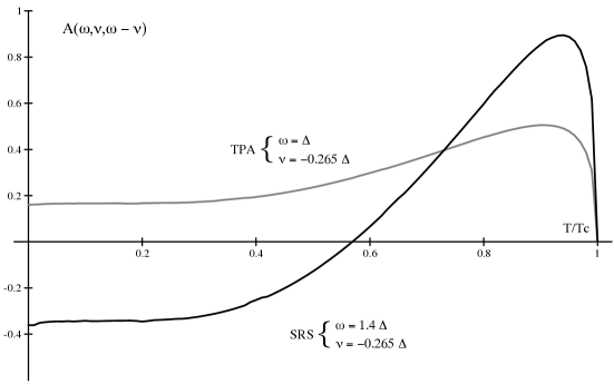
Figure 5.3: The temperature dependence of the nonlinear coupling constant $\tilde{A}(\omega,\nu,\omega-\nu)$ for $\omega-\nu=\sqrt{8/5}\Delta$; a) $\omega=\Delta$ (two-phonon absorption), b) $\omega=1.4\Delta$ (stimulated Raman scattering).

The angular dependence of $\Upsilon^{\pm}_{M}$ is determined by $Z_{M}(\hat{\bm{q}}_{1},\hat{\bm{q}}_{2})$ given in Eq. (5.137), which in turn depends on $\hat{\bm{z}}$, the quantization axis of the modes. This direction is determined by the relative size of the Zeeman energy, $\gamma H$, and the collective mode dispersion energy $Q_{\pm}\equiv v_{f}^{2}({\bm{q}}_{1}\pm{\bm{q}}_{2})^{2}/\Delta$. If $Q_{\pm}\gg\gamma{H}$ then $\hat{\bm{z}}$ is parallel to ${\bm{q}}_{1}\pm{\bm{q}}_{2}$, while if $Q_{\pm}\gg\gamma{H}$, then $\hat{\bm{z}}$ is parallel to the “rotated” magnetic field $\underline{{\bm{R}}}(\hat{\bm{n}},\theta)\cdot{\bm{H}}$. The angular dependence reduces to a simple form when the two wavevectors are either parallel or antiparallel,

$$|Z_{M}(\hat{\bm{q}},\pm\hat{\bm{q}})|^{2}=\frac{8\pi}{135}|{{\cal Y}_{2M}(\hat{\bm{q}})}|^{2}\,,$$ (5.195)

where ${\cal Y}_{2M}(\hat{\bm{q}})$ is a spherical harmonic. For $\hat{\bm{q}}=\pm\hat{\bm{z}}\,|\,Z_{M}\,|^{2}={{2}\over{27}}\,\delta_{M,0}$.

The sizes of the anomalies in the sound velocity and attenuation depend on the magnitudes of $\Upsilon^{\pm}_{M}$ and $\Gamma$. The height of the attenuation peaks increases linearly with $\Upsilon^{\pm}_{M}/\Gamma$ provided that $\Gamma\ll\Gamma_{d}$. Clearly $\Upsilon^{\pm}_{M}/\Gamma$ will be largest for large pump wave energy densities, low pressures (where $F_{0}^{s}$ and $\Gamma$ are smallest) and low temperatures, where $\Gamma$ is small. However, when the ratio $\Upsilon^{\pm}_{M}/\Gamma$ becomes sufficiently large that $\Gamma$ is comparable to the dispersion width $\Gamma$ the heights of the attenuation peaks tend to limiting values and their widths increase as $\Upsilon^{\pm}_{M}$ increases.

The damping of the order parameter collective modes due to quasiparticle collisions. $\Gamma$ is an increasing function of pressure and temperature. The expression for $\Gamma$ derived by Wölfle [74] depends in a complicated way on the quasiparticle scattering amplitudes, which are not well known. However, the lifetime of the modes, $1/\Gamma$, is roughly determined by the quasiparticle lifetime, $\tau$, which at very low temperatures $(T\ll T_{c})$ can be written

$$\frac{1}{\tau}=A(P)\,\left(\frac{T_{c}}{T}\right)^{3/2}\,e^{-\Delta/T}\,,$$ (5.196)

where $A$ is a function of pressure [19]. Although this expression is not valid at higher temperatures it is sufficiently accurate for the semi-quantitative results required here. We assume that the pressure dependence of $A(P)$ is that of $1/\tau_{N}$, where $\tau_{N}$ is the quasiparticle lifetime in the normal state,

$$\frac{1}{\tau_{N}}=\frac{(T/\mbox{mK})^{2}}{0.6-0.01\,P}\,,$$

where $P$ is the pressure in bars [19]. Thus, we assume

$$A(P)=\frac{A_{0}\,(T_{c}/\mbox{mK})^{2}}{0.6-0.01\,P}\,,$$ (5.197)

where $A_{0}$ is determined by fitting Eq. (5.196) to the data given by Halperin [25] for the lifetime of the $J=2^{-}$ mode at 13 bar. Expressions (5.196) and (5.197) are used for the mode lifetime $\Gamma$ in the calculations discussed below. In general, as the pressure increases the nonlinear features in the temperature become smaller and broader.

The attenuation as a function of temperature, at zero pressure, for a sound wave of frequency $35.8\,\mbox{MHz}$ $(\hbar\omega_{1}/k_{\text{B}}T_{c}=1.87)$ in the presence of a parallel pump wave with frequency $3.26\,\mbox{MHz}$ $(\hbar\omega_{2}/k_{\text{B}}T_{c}=0.17)$ and energy density $U/U_{c}=0.1$ is shown in Fig. 5.4(a). The large central peak is due to the linear coupling of the $J=2^{+}$ mode to the higher frequency wave and occurs at a temperature $T_{0}$ such that $\sqrt{8/5}\,\Delta(T_{0})=\hbar\omega_{1}$. The two peaks to the left and right of the central peak are due to two-phonon absorption and the inverse Raman effect, respectively, and occur at temperatures $T_{+}\simeq 0.58T_{c}$ and $T_{-}\simeq 0.76T_{c}$, determined by $\sqrt{8/5}\,\Delta(T_{\pm})=\hbar(\omega_{1}\pm\omega_{2})$. The background attenuation is due to the linear coupling of sound to the $J=2^{-}$ mode, off-resonance.

Figure 5.4: The predicted temperature dependences at zero pressure of the attenuation/amplification (in units of $cm^{-1}$) of a signal zero-sound wave with frequency $\omega_{1}$ in the presence of a parallel pump wave of frequency $\omega_{2}$ and energy density $U=0.1\,U_{c}$; a) $\frac{\omega_{1}}{2\pi}=35.8\,\mbox{MHz}$, $\frac{\omega_{2}}{2\pi}=3.26\,\mbox{MHz}$, b) $\frac{\omega_{1}}{2\pi}=3.26\,\mbox{MHz}$, $\frac{\omega_{2}}{2\pi}=35.8\,\mbox{MHz}$. The peaks at $T/T_{c}\sim 0.58$ and $0.76$ in both cases are due to nonlinear resonances. The central peak at $T/T_{c}=0.68$ is the linear absorption from the $J=2^{+}$ mode.

The temperature dependence at zero pressure of the attenuation (amplification) of a sound wave with frequency $\frac{\omega_{1}}{2\pi}=3.26\,\mbox{MHz}$ in the presence of a pump wave with frequency $\frac{\omega_{2}}{2\pi}=35.8\,\mbox{MHz}$ and energy density $U/U_{c}=0.1$ is shown in Fig. 5.4(b). The peak at $T_{+}$ is again due to two-phonon absorption. However, amplification occurs for temperatures near $T_{-}$ because of stimulated Raman scattering: phonons of frequency $\omega_{2}$ decay into phonons with lower frequency $\omega_{1}$ and real squashons of frequency $\omega_{M}$. No absorption peak from the linear coupling of the $J=2^{+}$ mode to the low frequency $\omega_{1}$ wave appears in Fig. 5.4(b) because it occurs at a temperature $T_{2}$ (such that $\sqrt{8/5}\,\Delta(T_{2})=\hbar\omega_{2}$), which is larger than $0.8T_{c}$.

Figure 5.5: The predicted temperature dependence of $v(\omega,T)/c_{1}$, the change in phase velocity of a zero-sound wave due to linear and nonlinear coupling to the $J=2^{+}$ mode. All parameter values are the same as in Figs. 5.4(a) and (b).

Figures 5.5(a) and 5.5(b) show the changes in phase velocity of a zero sound wave of frequency $\omega_{1}$ due to its linear and nonlinear interaction with the $J=2^{+}$ modes in the presence of a parallel wave of high intensity $(U\simeq 0.1U_{c})$ and frequency $\omega_{2}$. In 5.5(a), $\omega_{1}/2\pi=35.8\,\mbox{MHz}\,(\hbar\omega_{1}/k_{\text{B}}T_{c}=1.87)$ and $\omega_{2}/2\pi=3.26\,\mbox{MHz}\,(\hbar\omega_{2}/k_{\text{B}}T_{c}=0.17)$, while these two frequencies are reversed in Fig. 5.5(b). The features at temperature $T_{+}\simeq 0.58T_{c}$ are due to two-phonon absorption by the $J=2^{+}$ mode. The features at $T_{-}\simeq 0.76T_{c}$ in Fig. 5.5(a) and (b) are due to the inverse Raman effect and stimulated Raman scattering, respectively. Note that in both Figs. 5.4 and 5.5 the sound frequencies have been chosen so that both nonlinear resonances appear in a reasonable temperature range and do not overlap with the large anomalies due to linear coupling to the $J=2^{-}$ mode or pair-breaking.

Although the sizes of the nonlinear absorption and velocity anomalies increase with the energy density of the pump wave, there are obvious constraints on the amount of sound energy that is desirable in an experiment. Just as the superfluid state is destroyed by a superflow with velocity larger than the depairing critical velocity, it is also destroyed by sound waves with amplitude larger than some critical value. We expect that this occurs when $U\approx U_{c}$. In addition the pump wave causes heating of the superfluid at a maximum rate

$$C_{p}\frac{dT}{dt}=2\,\alpha\,c\,U\,,$$ (5.198)

where $C_{p}$ and $dT/dt$ are the heat capacity and rate of temperature increase of the ³He, and $\alpha$, $c$, and $U$ are the attenuation, phase velocity and energy density of the pump wave. In an experiment the sound energy density must be sufficiently small that the cryostat can keep the superfluid at a fixed temperature during the period of time in which the sound waves propagate through the cell. In the large amplitude sound experiments in ³He-B of Polturak et al. [51], they used the measured heating rate and estimated the sound energy density to be about one percent of the superfluid condensation energy density, i.e. $U/U_{c}\simeq 0.01$. This may be a more realistic estimate than the value of $U/U_{c}=0.1$ used in Figs. 5.4 and 5.5, shown for illustrative purposes.

Figures 5.6(a) and (b) show the temperature dependence of the height of the attenuation peaks associated with two-phonon absorption for a pump wave of energy density of $0.01\,U_{c}$. Corresponding calculations for the Raman peaks are shown in Figs. 5.7(a) and (b). The Raman peaks are expected to be small for temperatures close to $0.6T_{c}$ because, as shown in Fig. 5.3(a), the coupling function vanishes near this temperature. The maximum attenuation due to the nonlinear coupling of sound to the $J=2^{+}$ modes is of order $1\,\rm{cm}^{-1}$ over a wide temperature range. Since changes in the attenuation of order $0.1\,\rm{cm}^{-1}$, and changes in the phase velocity of order one part in $10^{6}$ are detectable, these nonlinear anomalies should be observable for accessible pump-wave energy densities.

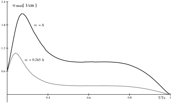
Figure 5.6: The temperature dependence at zero pressure of the peak in the signal wave attenuation due to two-phonon absorption by the $J=2^{+}$ mode for a pump wave of energy density $U=0.01\,U_{c}$ and a signal wave of frequency a) $\omega=\Delta$, and b) $\omega=0.265\Delta$.

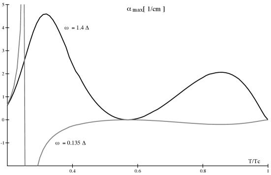
Figure 5.7: The predicted temperature dependence at zero pressure of a) the attenuation peak due to the inverse Raman effect for $\omega=1.4\Delta$, and b) the amplification peak due to stimulated Raman scattering for $\omega=0.135\Delta$. The pump wave energy density is $U=0.01\,U_{c}$.

5.7 Generation of third-harmonic and anti-Stokes waves

When we considered the three-wave resonance equations in the quasi-steady-state approximation, we noted that in addition to the terms in the nonlinear stress tensor with the frequency of the pump wave, $\omega_{1}$, and the Stokes wave, $\omega_{2}$, there are also oscillations with frequencies $2\omega_{1}-\omega_{2}$ and $2\omega_{2}-\omega_{1}$ which generate sound waves with the same frequencies. The analogous waves in nonlinear optics are known as anti-Stokes waves. These waves have much lower intensity than the pump wave and Stokes wave, which is why we neglected them earlier. Nevertheless, the anti-Stokes waves may be observable if the sound path is sufficiently short to reduce the destructive interference caused by dispersion. Our discussion is similar to Yariv’s treatment (Ref. [76], p. 421) of the effect of dispersion on optical second-harmonic generation.

The term in the nonlinear stress tensor with frequency $\omega_{a}=2\omega_{1}-\omega_{2}$ and wave vector $2{\bm{q}}_{1}-{\bm{q}}_{2}$ is

$$\delta\Pi_{a}({\bm{x}},t)=\chi_{a}\left[\tilde{N}_{1}({\bm{x}},t)\right]^{2}\,\tilde{N}_{2}({\bm{x}},t)^{*}\,,$$ (5.199)

where

$$\chi_{a} = \frac{1}{N(E_{f})^{2}(1+F_{0}^{s})\Delta^{2}}\left(\frac{c_{1}q_{1}}{\omega_{1}}\right)^{2}$$ (5.200)

$$\times \sum_{M}\,\frac{A_{M}(2\omega_{1}-\omega_{2},\omega_{1},\omega_{1}-\omega_{2})\,A_{M}(\omega_{1},\omega_{2},\omega_{1}-\omega_{2})^{*}}{\phi_{M}({\bm{q}}_{1}-{\bm{q}}_{2},\omega_{1}-\omega_{2})}\,.$$

The density oscillation generated by this driving term,

$$\delta{n}({\bm{x}},t)=N_{a}({\bm{x}},t)\,e^{-i(\omega_{a}t-{\bm{q}}_{a}\cdot{\bm{x}})}\,,$$ (5.201)

satisfies the wave equation

$$\left(\mbox{$\displaystyle\frac{\partial^{2}}{\partial t^{2}}$}-c_{1}^{2}\nabla^{2}\right)\delta{n}=2\,c_{1}^{2}\nabla^{2}\,\big{[}\delta\Pi_{a}+\delta\Pi_{L}\big{]}\,,$$ (5.202)

where $\delta\Pi_{L}$ is the contribution to the stress tensor from the linear coupling of the anti-Stokes wave to the collective modes. In the slowly varying envelope approximation the anti-Stokes wave obeys

$$\mbox{$\displaystyle\frac{\partial N_{a}}{\partial z}$}=iq_{a}\,\chi_{a}\,\left[\tilde{N}_{1}\right]^{2}\,\tilde{N}_{2}^{*}\,e^{i\Delta{q}z}\,,$$ (5.203)

where $\Delta q\equiv q_{a}-2q_{1}+q_{2}$ and $\omega_{a}=v(\omega)\,q_{a}$ where $v(\omega)$ is the frequency-dependent phase velocity for sound in the linear response limit. For frequencies away from the $J=2^{+}$ collective mode resonances the dispersion is dominated by the contributions from the excitations and off-resonant $J=2^{-}$ collective mode, and is given by

$$\frac{v(\omega)}{c_{1}}-1=\mbox{Re}\left(\frac{\delta\Pi_{L}}{\delta{n}}\right)=\frac{6\lambda(\omega)}{25(1+F_{0}^{s})}\,\frac{(\omega^{2}-4\Delta^{2})}{(\omega^{2}-12\Delta^{2}/5)}\,,$$ (5.204)

from Eq. (5.4). The wave-vector mismatch

$$\Delta{q}=\omega_{2}\left(\frac{1}{v(\omega_{2})}-\frac{1}{v(\omega_{a})}\right)-2\omega_{1}\left(\frac{1}{v(\omega_{1})}-\frac{1}{v(\omega_{a})}\right)\,,$$ (5.205)

is then nonzero because of dispersion. In order to integrate Eq. (5.203) we assume that the sound path is sufficiently short, that the attenuation of the pump and Stokes waves is sufficiently small so that their amplitudes $\tilde{N}_{1}$ and $\tilde{N}_{2}$ are nearly constant, and that the boundary condition for the anti-Stokes wave is $N_{a}(0)=0$. The solution is

$$N_{a}(z)=q_{a}\chi_{a}\,\tilde{N}_{1}(0)^{2}\,\tilde{N}_{2}(0)\,\frac{\left(e^{i\Delta{q}z}-1\right)}{\Delta{q}}\,.$$ (5.206)

and the relative intensity of the anti-Stokes wave to the Stokes wave is

$$\frac{I_{a}(z)}{I_{2}}=|{Gz}|^{2}\,J_{0}\bigg{(}{{1}\over{2}}\Delta{q}z\bigg{)}^{2}\,,$$ (5.207)

where $J_{0}(x)=\sin(x)/x$ is the zeroth-order spherical Bessel function, and $G=q_{a}\chi_{a}\tilde{N}_{1}(0)^{2}$. Thus, the anti-Stokes wave is destroyed by interference if the wave-vector mismatch or path length $L$ are sufficiently large, i.e. $\Delta{q}L\gg 1$. For frequencies $\omega_{1},\omega_{2}\sim\Delta$, the velocity mismatch is $[v(\omega_{1})-v(\omega_{2})]/c_{1}\sim 1/F_{0}^{s}$, so for low pressures, where $F_{0}^{s}$ is smallest, the wave-vector mismatch is relatively large, $\Delta{q}\sim 10\,\mbox{cm}^{-1}$. Thus, in order for anti-Stokes wave not to be destroyed by interference, the length of the sound path should be less than $1/\Delta{q}\simeq 1\,\mbox{mm}$.

The amplification of the Stokes wave was shown to be about $1\,\mbox{cm}^{-1}$ for a pump wave with energy density $0.1\,U_{c}$. Using this energy we estimate the relative intensities of the anti-Stokes and Stokes waves to be $I_{a}/I_{2}\simeq 10^{-3}$ for path lengths the order of a millimeter. Thus, although the Stokes wave is much larger than the anti-Stokes wave it may still be observable, provided it is not overdamped. If $\omega_{1}>\omega_{2}$ then the condition for stimulated Raman scattering, $\omega_{1}-\omega_{2}\simeq\sqrt{8/5}\Delta$, implies that $\omega_{a}>2\Delta$, and consequently the anti-Stokes wave would be strongly attenuated by pair breaking. On the other hand, if $\omega_{2}>\omega_{1}$ and $\omega_{2}-\omega_{1}\simeq\sqrt{8/5}\Delta$, then the anti-Stokes wave is not damped by pair breaking.

The generation of third harmonics is similarly limited by dispersion. Serene [65] has noted that the $J=2^{+}$ modes can give rise to a significant third-harmonic of the density. If there is a high-intensity sound wave, with frequency $\omega_{1}$ and wave vector ${\bm{q}}_{1}$,

$$\delta{n}({\bm{x}},t)=\tilde{N}_{1}({\bm{x}},t)\,e^{-i(\omega_{1}t-{\bm{q}}_{1}\cdot{\bm{x}})}\,,$$ (5.208)

whose second harmonic is resonant with the $J=2^{+}$ modes (i.e. $2\omega\simeq\sqrt{8/5}\Delta$), then in the quasi-steady-state approximation the amplitudes of these modes are given by

$$D^{+}_{2,M}({\bm{x}},t)=\frac{A_{M}(\omega_{1},-\omega_{1},2\omega_{1})}{N(E_{f})^{2}\,\Delta\,\phi^{M}(2{\bm{q}}_{1},2\omega_{1})}\left|\frac{c_{1}q_{1}}{\omega_{1}}\right|^{2}\Big{[}\tilde{N}_{1}({\bm{x}},t)\Big{]}^{2}+\mbox{c.c.}\,.$$ (5.209)

If this amplitude is inserted into the nonlinear stress tensor given by Eq. (5.163), together with Eq. (5.208), then a third-harmonic (frequency $3\omega_{1}$ and wavevector $3{\bm{q}}_{1}$) is obtained,

$$\delta\Pi({\bm{x}},t)=\chi_{3}\Big{[}\tilde{N}_{1}({\bm{x}},t)\Big{]}^{3}\,,$$ (5.210)

where

$$\chi_{3}=\negthickspace\negmedspace\sum_{M}\frac{1}{N(E_{f})^{2}\,(1+F_{0}^{s})\,\Delta^{2}}\negthickspace\negmedspace\left|\frac{c_{1}q_{1}}{\omega_{1}}\right|^{2}\negthickspace\negmedspace\left[\frac{A_{M}(3\omega_{1},\omega_{1},2\omega_{1})A_{M}(\omega_{1},-\omega_{1},2\omega_{1})^{*}}{\phi_{M}(2{\bm{q}}_{1},2\omega_{1})}\right].$$ (5.211)

Repeating the analysis of the of the relative intensity of the anti-Stokes waves for the third-harmonic, it follows that the ratio of the intensity of the third harmonic to that of the first harmonic is given by

$$\frac{I_{3}(z)}{I_{1}}=\left|G_{3}z\right|^{2}\,J_{0}\bigg{(}{{1}\over{2}}\Delta{q}z\bigg{)}\,,$$ (5.212)

where the wave-vector mismatch is $\Delta{q}=q_{3}-3q_{1}$, and $G_{3}=q_{3}\chi_{3}\,N_{1}(0)^{2}$. We estimate that for the third harmonic not to be destroyed by the interference, the sound path must be shorter than $1/\Delta{q}\simeq 1\,\mbox{mm}$, as in the case of the anti-Stokes wave. Similarly, for reasonable values of parameters the intensity of the third harmonic is estimated to be $I_{3}/I_{1}\simeq 10^{-4}$. Although the neglect of the third harmonic in the previous section was justified it may also be of sufficient intensity to be observable. However, in practice it may be difficult to distinguish the third harmonic signal generated by the nonlinear response of the superfluid from the signals generated by the nonlinearities in the experimental apparatus [65].

The results presented here for third-harmonic generation differ from those of Serene in two respects; (i) here we consider the detrimental effect of dispersion on the third-harmonic signal, and (ii) Serene’s estimates for the nonlinear coupling constants are several orders of magnitude larger than those presented here. This discrepancy has been resolved. Serene [66] did not evaluate the complicated integral he obtained for the coupling to the third harmonic, rather he assumed the properly scaled integral to be of order unity. However, Kopp [33] has evaluated the integral in Serene’s paper and shown that it vanishes to leading order in $1/s^{2}\sim 1/F_{0}^{s}$. The method used here to derive the collective mode equations shows that this cancellation to leading-order in $1/s^{2}$ is a consequence of gauge and Galilean invariance.

5.8 Conclusion

We have attempted to give a reasonably complete discussion of the relationship of collisionless sound propagation and attenuation to the order parameter collective modes of superfluid ³He-B. These modes, which reflect the symmetries of the normal state as well as the broken gauge and relative rotational symmetries of the condensate, play a central role in the high-frequency response of the superfluid. The acoustic spectroscopy based on the linear coupling of the $J=2^{\pm}$ modes is well developed. The Zeeman effect for both sets of $J=2$ modes has been observed, as well as the effects of gap distortion and textures on the attenuation and velocity spectra of sound. Measurements of the temperature and field dependences of the $J=2^{\pm}$ modes have been used to obtain quantitative results for the gap as well as the quasiparticle interactions that renormalize the collective mode frequencies. In short, the linear response is fairly well understood.

Much less is known about the nonlinear acoustic response of superfluid ³He. We have presented the underlying theory, based on the quasiclassical equations of superfluid ³He, of the weak nonlinear response of superfluid ³He-B for the case of a three-wave resonance between two sound waves of different frequencies and the $J=2^{\pm}$ modes, as well as the generation of higher harmonic sound waves. The $J=2^{+}$ modes couple nonlinearly to two zero-sound waves even though exact particle-hole symmetry of the normal Fermi liquid is built into the quasiclassical equations. The predictions for the nonlinear absorption and velocity anomalies resulting from the $J=2^{+}$ modes depend on relatively well understood material properties of ³He.

Acknowledgements

We thank our colleagues Bill Halperin, Thilo Kopp, John Ketterson, Dierk Rainer and Joe Serene for their many insights and helpful comments on sound propagation, collective modes and the quasiclassical theory of superfluid ³He.

5.9 Corrections to the Published Manuscript

1. The labeling of the Nambu matrices in Eq. 5.43 is corrected from $\mu=\{1,2,3,4\}$ to $\mu=\{0,1,2,3\}$.

2. Sign in Eq. 5.56 is corrected: $+\eta\rightarrow-\eta$.

3. Added subscript to Eq. 5.60.

4. In the line above Eq. 5.86, the corrected sentence reads: “… for $\sigma_{a}\neq\varepsilon^{+}$ (i.e. $a\neq 1$) …”.

5. In the sentence above Eq. 5.92, the corrected sentence reads, “… local spin rotations generated by $\hat{\Lambda}={\bm{\theta}}\cdot\hat{{\bm{\Sigma}}}$ …”.

6. Corrected coupling strength in Eq. 5.4: $\zeta(\omega)\rightarrow[\zeta(\omega)]^{2}$.

7. Corrected Eq. 5.5 line 1: $A(\omega,\nu,\omega-\nu)=-4\Delta^{2}\ldots$.

8. Corrected Eq. 5.5 line 5: $E(\omega,\nu,\omega-\nu)=\frac{-2}{\nu\Delta}\ldots$.

9. In the 2nd line of Eq. 5.159, $P_{2}(\hat{\bm{p}},\hat{\bm{s}})\rightarrow P_{2}(\hat{\bm{p}}\cdot\hat{\bm{s}})$.

10. Corrected Eq. 5.163 to agree with Eq. 5.25, which is the correct form.

11. Corrected the RHS of the 2nd line of Eq. 5.5: $A_{M}(\omega_{2},-\omega_{1},\omega_{2})$ $\rightarrow$ $A_{M}(\omega_{2},-\omega_{1},\omega_{3})$.

12. In Eq. 5.208: $e^{-(i\omega_{1}-{\bm{q}}_{1}\cdot{\bm{x}})}$ $\rightarrow$ $e^{-i(\omega_{1}t-{\bm{q}}_{1}\cdot{\bm{x}})}$.

Bibliography

[1]
Allen, L. and Eberly, J. H. (1975)).
Optical Resonance and Two Level Atoms.
Wiley, New York.
[2]
Ambegaokar, V. and Kadanoff, L. P. (1961).
Electromagnetic properties of superconductors.
Nuovo Cimento, 22, 914.
[3]
Anderson, P. W. (1958).
Coherent Excited States in the Theory of Superconductivity: Gauge
Invariance and the Meissner Effect.
Phys. Rev., 110(4), 827–835.
[4]
Anderson, P. W. (1958).
Random-Phase Approximation in the Theory of Superconductivity.
Phys. Rev., 112(6), 1900–1916.
[5]
Avenel, O., Piche, L., Rouff, M., Varoquaux, E., Combescot, R., and Maki, K.
(1985).
The Acoustic Impedance of Superfliud 3He-B.
Phys. Rev. Lett., 54, 1408.
[6]
Avenel, O., Varoquaux, E., and Ebisawa, H. (1980).
Field Splitting of the New Sound Attenuation Peak in 3He-B.
Phys. Rev. Lett., 45, 1952.
[7]
Balian, R. and Werthamer, N. R. (1963).
Superconductivity with Pairs in a Relative P-state.
Phys. Rev., 131, 1553.
[8]
Bardeen, J. (1961).
Quantization of Flux in a Superconducting Cylinder.
Phys. Rev. Lett., 7, 162–163.
[9]
Baym, G. and Pethick, C. J. (1978).
The Physics of Solid and Liquid Helium, Part 2, pp. 1–122.
Wiley, New York.
[10]
Bloembergen, N. (1965).
Non-linear Optics.
Benjamin, Reading.
[11]
Bogoliubov, N. N., Tolmachev, and Shirkov (1958).
New Methods in the Theory of Superconductivity.
Academy of Science, Moscow.
[12]
Brusov, P. N. and Popov, V. N. (1980).
Stability of the Bose Spectrum of Superfluid Systems of the 3He
Type.
Zh. Eskp. Teor. Fiz., 78, 2419.
[JETP, 51, 117 (1980)].
[13]
Bunkin, F. V., Kravstov, Yu. A., and Lyakhov, G. A. (1986).
Acoustic Analogues of Nonlinear-Optics Phenomena.
Sov. Phys. Usp., 29, 607.
[14]
Carlson, R. V. and Goldman, A. M. (1975).
Propagating Order-Parameter Collective Modes in Superconducting
Films.
Phys. Rev. Lett., 34, 11.
[15]
Combescot, R. (1982).
Dispersion Relations of the High-Frequency Modes in 3He-B.
J. Low Temp. Phys., 49, 295.
[16]
Daniels, M. E., Dobbs, E.R., Saunders, J., and Ward, P.L. (1983).
Observation of New Structure in the Collective Mode Spectrum of Zero
Sound in 3He-B.
Phys. Rev. B, 27, 6988.
[17]
Eckern, U. (1981).
Quasiclassical Approach to Kinetic Equations for Superfluid 3He:
General Theory and Application to the Spin Dynamics.
Ann. Phys., 133, 390.
[18]
Eilenberger, G. (1968).
Transformation of Gorkov’s Equation for Type II Superconductors into
Transport-Like Equations.
Zeit. f. Physik, 214, 195.
[19]
Einzel, D. (1984).
Spin-independent Transport Parameters for Superfluid 3He-B.
J. Low Temp. Phys., 54, 427.
[20]
Eliashberg, G. M. (1972).
Inelastic Electron Collisions and Nonequilibrium Stationary States
in Superconductors.
Sov. Phys. JETP, 34, 668.
[Zh. Eskp. Teor. Fiz., 61, 1254 (1971)].
[21]
Fishman, R. S and Sauls, J. A (1985, Jan).
Particle-Hole Symmetry Violation in Normal Liquid .
Physical Review B, 31(1), 251–259.
[22]
Fishman, R. S. and Sauls, J. A. (1986).
Response Functions and Collective Modes of Superfluid -B in
Strong Magnetic Fields.
Phys. Rev. B, 33, 6068.
[23]
Fisk, Z., Hess, D.W., Pethick, C.J., Pines, D., , Smith, J.L., Thompson, J.,
and Willis, J.O. (1988).
Heavy-Electron Metals: New Highly Correlated States of Matter.
Science, 239, 33.
[24]
Giannetta, R. W., Ahonen, A., Polturak, E., Saunders, J., and Zeise, E. K.
(1980).
Observation of a New Sound Attenuation Peak in Superfliud 3He-B.
Phys. Rev. Lett., 45, 262.
[25]
Halperin, W. P. (1982).
Acoustic Order Parameter Mode Spectroscopy in Superfluid 3He-B.
Physica, 109-110B, 1596.
[26]
Halperin, W. P. and Varoquaux, E. (1990).
Order Parameter Collective Modes in Superfluid .
In Helium Three (ed. W. P. Halperin and L. P. Pitaevskii), p.
353. Elsevier Science Publishers, Amsterdam.
[27]
Kaup, D. J., Reiman, A., and Bers, A. (1979).
Space-time evolution of nonlinear three-wave interactions. I.
Interaction in a homogeneous medium.
Rev. Mod. Phys., 51, 275.
[28]
Keldysh, L. V. (1965).
Diagram Technique for Nonequilibrium Processes.
Sov. Phys. JETP, 20, 1018.
[29]
Ketterson, J. B. (1983).
Coupling of Spin Waves to Zero Sound.
Phys. Rev. Lett., 50, 259.
[30]
Kieselmann, G. and Rainer, D. (1983).
Branch Conversion at Surfaces of Superfluid 3He.
Z. Phys., B52, 267.
[31]
Koch, V. E. and Wölfle, P. (1981).
Coupling of New Order Parameter Collective Modes to Sound Waves in