UAV Circumnavigation of an Unknown Target Without Location Information Using Noisy Range-based Measurements

Abstract

This paper proposes a control algorithm for a UAV to circumnavigate an unknown target at a fixed radius when the location information of the UAV is unavailable. By assuming that the UAV has a constant velocity, the control algorithm makes adjustments to the heading angle of the UAV based on range and range rate measurements from the target, which may be corrupted by additive measurement noise. The control algorithm has the added benefit of being globally smooth and bounded. Exploiting the relationship between range rate and bearing angle, we transform the system dynamics from Cartesian coordinate in terms of location and heading to polar coordinate in terms of range and bearing angle. We then formulate the addition of measurement errors as a stochastic differential equation. A recurrence result is established showing that the UAV will reach a neighborhood of the desired orbit in finite time. Some statistical measures of performance are obtained to support the technical analysis.

I Introduction

Unmanned Aerial Vehicles (UAVs) have been rapidly developing in capability and hold promise for private, military, and even commercial uses. From the transport of small goods in rural areas to the early detection of forest fires [1], UAVs will likely be a ubiquitous tool in coming years. However, navigation of UAVs is heavily dependent on the use of GPS signals for location information. Recent tests show that UAVs are vulnerable to GPS jamming and spoofing, as evidenced by [2], [3]. Hence, it is desirable to develop autonomous control schemes under GPS-denied environment.

A typical application of UAVs is to gather information from a target. In order to obtain enough information regarding a target, it is often necessary to have the UAV orbit around this target at some predetermined distance. Such a UAV motion is often called circumnavigation. While some study has been devoted to the circumnavigation mission, most control techniques use some type of location information. In [4], the GPS coordinate of the target is considered unknown but the location information of the UAV under some local coordinate frame is assumed to be available. Range measurements from the target are then used to localize the target; that is, to estimate the relative location of the target from the UAV. A control algorithm is then designed to produce the desired UAV motion. In [5], the dynamics are modeled differently which allows the use of the bearing angle for target localization, but the location information of the UAV under some local coordinate frame is still assumed.

In [6], Cao et al. exploited a trigonometric relationship in the system dynamics that allows the range rate to be used as a proxy for the bearing angle. It also enables one to transform the UAV dynamics from Cartesian to polar coordinates, reducing the state space from the 2D location plus the heading angle to simply the range and bearing angle. Control algorithms were then developed which use range and range rate measurements to drive the UAV to the desired orbit without the need for target localization nor the knowledge of the UAV’s current position. Clearly, this is advantageous in situations where GPS is unreliable or unavailable.

In this paper, we expand on the above work to develop a control algorithm for the circumnavigation task using noisy range and range rate measurements. In [6], two different control algorithms were developed; one is smooth but unsaturated, while the other is saturated but nonsmooth. Both control algorithms were defined only outside the desired orbit, meaning that zero control input is applied on the inside of the desired orbit to force the UAV to fly straight until it exits again. To improve the performance we develop a new control algorithm which is both smooth and saturated via introducing an appropriate control policy for inside the desired orbit. In addition, a recurrence result can be established; meaning that the UAV will reach a neighborhood of the desired orbit in finite time, and return if it deviates away from the neighborhood. We then employ numerous examples show the robustness of the new algorithm against measurement noise as well as wind because only range-based measurements are needed.

The rest of the paper is organized as follows. Section II describes the assumed dynamics and the relations used in the development of the control. Section III motivates and develops a new control policy based on range and range rate measurements; first by examining when the UAV is outside of a given ‘singular’ orbit corresponding to the choice of one parameter in the control algorithm, and then by examining when the UAV is inside the singular orbit. Section IV focuses on analyzing the effect of noisy range and range rate measurements on the proposed control algorithm by means of stochastic differential equations (SDEs). A recurrence result is then established, deriving an upper bound on the time for the UAV to reach some neighborhood of the desired orbit. Finally, Section V presents a simulation study of the performance of the control algorithm with noise-corrupted measurements and collect performance statistics for varying choices of the gain size. Then the effect of constant wind is simulated to demonstrate the robustness of the control algorithm when the gain is appropriately large. Finally, Section VI summarizes the paper and outlines directions for future work.

II Probem Formulation

The problem set-up is as follows. Assuming the UAV travels at a constant velocity $V$, the dynamics are given by

$$\begin{aligned} \dot{x}&=V\cos(\psi)\\ \dot{y}&=V\sin(\psi)\\ \dot{\psi}&=u\end{aligned}$$ (1)

where $[x,y]$ is the 2D location of the UAV, $\psi$ is the heading angle of the UAV, and $u$ is the heading rate to be controlled. The objective is to design a control algorithm for $u$ such that the UAV orbits some unknown stationary target at a desired radius $r_{d}$. Considering limited measurements available under GPS-denied environment, the controller has to be constructed based on range measurement $r(t)$ and range rate measurement $\dot{r}(t)$. Here $r(t)$ refers to the distance from the UAV to the target and $\dot{r}$ refers to the rate of $r(t)$.

Figure 1: Heading angle $\psi$ vs. bearing angle $\theta$ vs. reference angle $\phi$.

For the convenience of notation, we take the target $T$ as the origin of our coordinate frame. To design a control algorithm and carry out the analysis we shall make use of the reference angle $\phi$ to the UAV, as well as the local heading angle $\psi$ of the UAV and the bearing angle $\theta$ from the reference vector to the heading vector. See Figure 1 for a depiction. We note that

$$\begin{aligned} \theta=\pi-\phi+\psi.\end{aligned}$$ (2)

Then observing

$$\begin{aligned} \dot{r}&=\frac{1}{\sqrt{x^{2}+y^{2}}}\left[x\dot{x}+y\dot{y}\right]=\cos(\phi)\dot{x}+\sin(\phi)\dot{y},\end{aligned}$$ (3)

using the dynamics for $\dot{x}$ and $\dot{y}$ given by (1), and applying $\phi=\pi-\theta+\psi$ we arrive at

$$\begin{aligned} \dot{r}=-V\cos\theta.\end{aligned}$$ (4)

Thus there is a direct correspondence between the bearing angle $\theta$ and the range rate $\dot{r}$. This fundamental relation will allow us to use $\dot{r}$ as a proxy for $\theta$ to design our control.

Also, $\dot{\theta}=-\dot{\phi}+\dot{\psi}=-\dot{\phi}+u$, where

$$\begin{aligned} \dot{\phi}&=\frac{\cos(\phi)\dot{y}-\sin(\phi)\dot{x}}{\sqrt{x^{2}+y^{2}}}=-\frac{V}{r}\sin\theta\end{aligned}$$ (5)

so we can transform the system dynamics from $\{(x,y,\phi)\}$ in (1) to $\{(r,\theta)\}$ given by

$$\begin{aligned} \dot{r}&=-V\cos\theta\\ \dot{\theta}&=\frac{V\sin\theta}{r}+u\end{aligned}$$ (6)

The goal is to design a control $u(r,\dot{r})=u(r,-V\cos\theta)$ such that the dynamics drive $(r,\theta)$ to $(r_{d},\frac{\pi}{2})$.

III The Control Algorithm

The designed control algorithm is composed of two cases: (1) $r\geq r_{s}$; and (2) $r<r_{s}$, where $r_{s}<r_{a}$ is a positive constant defined next. The following two subsections detail how control algorithm is developed for the two cases.

III-A Outer Control

Suppose that $r\geq r_{s}$, i.e., the UAV is outside of the black circle as in Figure 2. The idea for the control algorithm is to drive the UAV towards the tangent point (from the UAV) of the black circle. There is a need to distinguish between the black circle which is being aimed for and the ‘actual’ red circle that is achieved, because we shall see that they are not the same (though an explicit relationship between them can be identified based on the controller proposed next). Letting $\gamma=\sin^{-1}\left(\frac{r_{s}}{r}\right)$, we want to adjust $\psi$ so that $\theta=\gamma$. Without the ability to measure $\psi$, it is not possible to make a direct adjustment. If $\dot{r}$ is measurable, it can serve as a proxy for $-V\cos\theta$. Given a preference that the UAV orbit clockwise (so that $\theta,\gamma\in[0,\pi]$), $\cos(\cdot)$ is decreasing on $[0,\pi]$. It then can be obtained that

$$-(\cos\theta-\cos\gamma)=\cos\gamma-\cos\theta=\Big{\{}\begin{array}[]{l r}\leq 0&\theta\geq\gamma\\ \geq 0&\theta\leq\gamma\end{array}$$

and thus

$$\begin{aligned} &-k\left[\dot{r}+V\cos\sin^{-1}\frac{r_{s}}{r}\right]\\ &=kV\left[\cos\theta-\cos\gamma\right]=\Big{\{}\begin{array}[]{lcr}<0&\text{for}&\theta>\gamma\\ >0&\text{for}&\theta<\gamma\end{array}.\end{aligned}$$ (7)

This motivates us to define a control for outside $r_{s}$ by

$$\begin{aligned} u_{o}(r,\dot{r})&=-k\left[\dot{r}+V\cos\sin^{-1}\left(\frac{r_{s}}{r}\right)\right]\mathbb{I}_{\{r\geq r_{s}\}},\\ &\qquad\ \text{ or equivalently }\\ u_{o}(r,\theta)&=\left[kV\cos\theta-kV\frac{\sqrt{r^{2}-r_{s}^{2}}}{r}\right]\mathbb{I}_{\{r\geq r_{s}\}}\end{aligned}$$ (8)

where $k$ is a positive constant. Note that the control is bounded by $2kV$.

Figure 2: We design a control which aims at the tangent of the orbit of radius $r_{s}$, but will ‘stabilize’ at the orbit of radius $r_{a}$. Here, $\gamma=\sin^{-1}(r_{s}/r)$.

Interestingly, the UAV cannot stabilize at an orbit of radius $r_{s}$. Assuming a stable circular orbit exists with its radius $r_{a}$, by definition, $\dot{r}=0$. The nominal angular velocity $|\frac{V}{r_{a}}|=|\dot{\psi}|=|u(r_{a},0)|$, indicating that

$$\begin{aligned} &\frac{V}{r_{a}}=kV\cos\sin^{-1}\left(\frac{r_{s}}{r_{a}}\right)=kV\frac{\sqrt{r_{a}^{2}-r_{s}^{2}}}{r_{a}}\\ &\implies\frac{1}{k^{2}}=r_{a}^{2}-r_{s}^{2}.\end{aligned}$$ (9)

Thus, given any desired actual orbit $r_{d}$, one may choose a gain size $k\in[\frac{1}{r_{d}},\infty)$ and obtain the parameter $r_{s}=\sqrt{r_{d}^{2}-\frac{1}{k^{2}}}$ for the control algorithm (8) such that a stable orbit of radius $r_{d}$ is feasible. From here throughout, we set $r_{a}=r_{d}$ so that the actual orbit is equal to the desired orbit, and take $r_{s}$ as defined by (LABEL:r_s-defn).

III-B Inner Control

When $r<r_{s}$, (8) is not well defined due to the term $\cos\sin^{-1}\left(\frac{r_{s}}{r}\right)$. So a new controller is needed for inside the black circle in Figure 2. In [6], zero control input is applied in order to drive the UAV outside the black circle. One disadvantage of such a control strategy (i.e., zero control for inside the black circle) is that the UAV has to move outside the black circle before control takes affect. As shown in Figure 4, the performance is degraded if the UAV moves inside the black circle quite often. This is particularly true when range and/or range rate measurements are noisy and $r_{d}$ is close to $r_{s}$ for large $k$. To keep the UAV from crossing across the desired orbit, similar to the trajectory depicted in Figure 4, a new control algorithm is needed for this case.

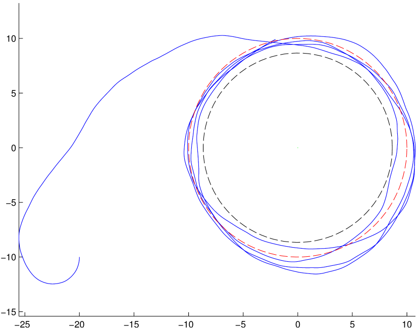
Figure 3: A sample trajectory under $u_{o}$ with small gain: $k=.2$, $r_{a}=10$, $r_{s}=8.67$, $V=1$, and additive white measurement noise $\sigma=0.5$.

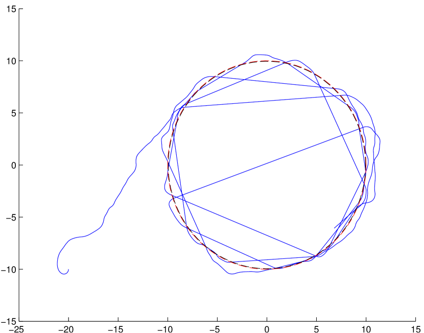
Figure 4: A sample trajectory under $u_{o}$, with large gain: $k=1$ corresponding to $r_{s}=9.95$. When measurement error nudges the UAV past the $r_{s}$ threshold, it cuts across the circle.

Note that the two terms in $u_{o}(r,\theta)=kV\cos\theta-kV\frac{\sqrt{r^{2}-r_{s}^{2}}}{r}$ work separately to adjust the bearing angle and radius. If $\theta<\frac{\pi}{2}$ (the bearing is too acute) then $kV\cos\theta$ is positive and drive the UAV counter clockwise, and does the reverse if $\theta>\frac{\pi}{2}$. And if $r>r_{s}$, then $\frac{-kV}{r}\sqrt{r^{2}-r_{s}^{2}}$ adjusts the heading in such a way that the UAV rotates toward heading the target. This suggests the following inner control as

$$\begin{aligned} u_{i}(r,\dot{r})&=-k\left[\dot{r}-\cos\sin^{-1}\left(\frac{r}{r_{s}}\right)\right]\mathbb{I}_{\{r<r_{s}\}}\\ u_{i}(r,\theta)&=\left[kV\cos\theta+\frac{kV}{r_{s}}\sqrt{r_{s}^{2}-r^{2}}\right]\mathbb{I}_{\{r<r_{s}\}},\end{aligned}$$ (10)

where the first component in (10) is the same as the first component in $u_{o}$, but the second component is negated with the nominator and denominator flipped.

Again, a stable orbit of radius $r_{i}<r_{s}$ is possible. If such an orbit exists, it must satisfy $|\frac{V}{r_{i}}|=|u_{i}(r_{i},0)|$. By computation, one can obtain

$$\begin{aligned} r_{i}^{2}&=\frac{1}{2}\left[r_{s}^{2}-\sqrt{r_{s}^{4}-\frac{4}{k^{2}}r_{s}^{2}}\right]\\ &=\frac{1}{2}\left(r_{a}^{2}-\frac{1}{k^{2}}\right)\pm\frac{1}{2}\sqrt{\left(r_{a}^{2}-\frac{1}{k^{2}}\right)\left(r_{a}^{2}-\frac{5}{k^{2}}\right)}.\end{aligned}$$ (11)

which has no solution for $k\in(\frac{1}{r_{a}},\frac{\sqrt{5}}{r_{a}})$, but otherwise has two solutions $r_{i-}\to 0$ and $r_{i+}\to r_{a}$ as $k\to\infty$. These will play some role in the recurrence analysis.

Remark 3.1:

We note that the UAV can only stabilize at one of the inner stable radii $r_{i}$ if the initial point and heading is exactly along the orbit with radius $r_{i}$ in a counter-clockwise orientation, corresponding to $(r(0),\theta(0))=(r_{i},3\pi/2)$, thus forcing the ‘$\theta$’ (or $\dot{r}$) component of the control $kV\cos\theta$ in (10) to be 0. However, any perturbation of the inputs for the control which force the UAV even negligibly off-course will cause the $\theta$ component to drive the UAV’s bearing angle towards $\pi/2$ because $(r_{i},3\pi/2)$ is an unstable equilibrium. Eventually, the UAV will be driven outside the orbit with radius $r_{s}$. In the presence of measurement errors, the UAV is driven outside the orbit with radius $r_{s}$ almost immediately as evidenced by Figure 6. Other simulations demonstrate that even if $(r(0),\theta(0))=(r_{i},3\pi/2)$ and no measurement errors exist, accumulated numerical errors will eventually drive the UAV slightly off the orbit of radius $r_{i}$ after which it immediately moves outside the orbit with radius $r_{s}$. Hence the inner stable orbits are of little practical concern for the implementation of the control algorithm.

As a summarization, the proposed control algorithm is given by $u=u_{o}+u_{i}$; that is

$$\begin{aligned} u(r,\dot{r})=&-k\dot{r}-kV\cos\sin^{-1}\left(\frac{r_{s}}{r}\right)\mathbb{I}_{\{r>r_{s}\}}\\ &+kV\cos\sin^{-1}\left(\frac{r}{r_{s}}\right)\mathbb{I}_{\{r<r_{s}\}}\end{aligned}$$ (12)

or equivalently

$$\begin{aligned} u(r,\theta)=&kV\cos\theta-\frac{kV}{r}\sqrt{r^{2}-r_{s}^{2}}\mathbb{I}_{r>r_{s}}\\ &+\frac{kV}{r_{s}}\sqrt{r_{s}^{2}-r^{2}}\mathbb{I}_{\{r<r_{s}\}}.\end{aligned}$$

As an example, Figures 6 and 6 depict the improved performance of the UAV under the proposed control algorithm (12) with $k=1$. Notice that the UAV will eventually stay close to the desired orbit as opposed to the behavior seen in Figure 4 when zero control is applied for the case $r(t)<r_{s}$.

Figure 5: A sample trajectory under $u$ with initial point outside the desired orbit

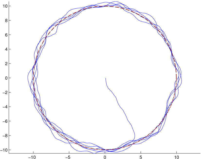
Figure 6: Sample trajectory under $u$ with initial point inside the desired orbit

IV Measurement Error Analysis

IV-A SDE Formulation

Here we formally introduce additive measurement noises in the controller. For example, range $r$ can be measured accurately, but range rate measurement is noisy $\widetilde{\dot{r}}=\dot{r}+\nu$ where $\nu\sim\mathcal{N}(0,\sigma)$. This model has practicality, as the range measurements are tremendously accurate compared to range rate measurements regardless of what method we use for the estimation. Then the noisy control input becomes

$$\widetilde{u}(r,\theta,\nu) \overset{\Delta}{=}u(r,\dot{r}+\nu)\overset{\Delta}{=}u(r,\theta)-k\nu.$$

With the noisy control input, the noisy system dynamics are modeled by the stochastic differential equation

$$\begin{aligned} d\left[\begin{array}[]{c}r\\ \theta\end{array}\right]=\left[\begin{array}[]{c}-V\cos\theta\\ \frac{V\sin\theta}{r}+u(r,\theta)\end{array}\right]dt+\left[\begin{array}[]{c}0\\ -k\sigma\end{array}\right]d\xi\end{aligned}$$ (13)

where $\xi$ is a standard Brownian motion. One can verify that the control defined by (12) has linear growth and is Lipschitz continuous (even at $r=r_{s}$), and the other coefficients also satisfy this property on domains bounded away from $r=0$. Hence (13) describes an Ito diffusion, and thus a unique Markov solution exists for the trajectory as in [8, Definition 7.1.1, Theorem 5.2.1]. The associated generator $\mathcal{L}$ of the diffusion is given by

$$\begin{aligned} &\mathcal{L}\mathcal{V}(r,\theta)=\left[-V\cos\theta\right]\frac{\partial}{\partial r}\mathcal{V}(r,\theta)\\ &+\left[\frac{V\sin\theta}{r}+u(r,\theta)\right]\frac{\partial}{\partial\theta}\mathcal{V}(r,\theta)+\frac{k^{2}\sigma_{rr}^{2}}{2}\frac{\partial^{2}}{\partial\theta^{2}}\mathcal{V}(r,\theta).\end{aligned}$$ (14)

IV-B A Recurrence Result

Let $Z(t)$ be an $\ell$-dimensional diffusion process. It is said to be regular if it does not blow up in finite time w.p.1. Suppose that $Z(t)$ is an $\ell$-dimensional diffusion process that is regular, that $D$ is an open set with compact closure, that $Z(0)=z\in D^{c}$ the complement of $D$, and that $\sigma^{z}_{D}=\inf\{t:Z^{z}(t)\in D\},$ where $Z^{z}(t)$ signifies the initial data $z$ dependence of the diffusion. The process $Z^{z}(\cdot)$ is recurrent with respect to $D$ if $P(\sigma^{z}_{D}<\infty)=1$ for any $z\in D^{c}$; otherwise, the process is transient with respect to $D$. A recurrent process with finite mean recurrence time for some set $D$ is said to be positive recurrent w.r.t. $D$; otherwise, the process is null recurrent w.r.t. $D$.

Coming back to our problem, we shall show that the trajectory of the UAV under control policy (12) with dynamics given by (13) is recurrent with respect to a neighborhood of either $r=r_{a}$ or $r=0$, as depicted in Figure 7. The recurrence is in the sense that if the initial point of the UAV is outside of the recurrent set, the UAV will enter the recurrent set in finite time almost surely.

Figure 7: The recurrent set $U_{k,\varepsilon}$.

We shall prove our result using a Lyapunov function approach. Consider the candidate function

$$\mathcal{V}(r,\theta)=\frac{k}{V}|r-r_{s}|+\frac{\theta}{V}{\operatorname{sgn}}(r-r_{s})+\frac{2\pi}{V}$$ (15)

which is everywhere positive on the domain $r\in(0,r_{s})\cup(r_{s},\infty)$ and $\theta\in[0,2\pi)$. Note that $\mathcal{V}$ by (15) is not differentiable along $r=r_{s}$. However, this will become part of the recurrent set $U_{k,\varepsilon}$ and it is only on the complement set $U_{k,\varepsilon}^{c}$ which the Lyapunov function must be smooth. On such a domain, we have that

$$\begin{aligned} \mathcal{L}\mathcal{V}&=-k\cos\theta{\operatorname{sgn}}(r-r_{s})+\frac{\sin\theta}{r}{\operatorname{sgn}}(r-r_{s})\\ &\qquad+k\cos\theta{\operatorname{sgn}}(r-r_{s})+u(r){\operatorname{sgn}}(r-r_{s})\\ &=\frac{\sin\theta}{r}{\operatorname{sgn}}(r-r_{s})-\frac{k}{r}\sqrt{r^{2}-r_{s}^{2}}\mathbb{I}_{\{r>r_{s}\}}\\ &\qquad\qquad\qquad-\frac{k}{r_{s}}\sqrt{r_{s}^{2}-r^{2}}\mathbb{I}_{\{r<r_{s}\}}.\end{aligned}$$ (16)

Theorem 4.1:

For $\varepsilon$ sufficiently small and $k$ sufficiently large, there exists

$$\begin{aligned} &r_{i-,\varepsilon}\searrow r_{i-}\quad&r_{i+,\varepsilon}\nearrow r_{i+}\qquad&r_{a,\varepsilon}\searrow r_{a}\quad&\text{ as }\varepsilon\downarrow 0\\ &\text{ where }&&&\\ &r_{i-}\searrow 0\quad&r_{i+}\nearrow r_{s}\qquad&r_{s}\nearrow r_{a}\quad&\text{ as }k\uparrow\end{aligned}$$ (17)

such that $\mathcal{L}\mathcal{V}\leq-\varepsilon$ on $U_{k,\varepsilon}^{c}$, where

$$\begin{aligned} U_{k,\varepsilon}\overset{\Delta}{=}&\{(0,r_{i-,\varepsilon})\times(\pi,2\pi)\}\cup\{(r_{i+,\varepsilon},r_{a,\varepsilon})\times(0,\pi)\}.\end{aligned}$$ (18)

With the above, using [7, Theorem 3.9], we can obtain the following corollary.

Corollary 4.2 (Recurrence Time Bound):

For $\varepsilon$ sufficiently small and $k$ sufficiently large, the trajectory of the UAV derived from (13) under control policy (12) is recurrent to $U_{k,\varepsilon}$ as defined in (18). Given an initial point $(r_{0},\theta_{0})$, the expected recurrence time $\tau_{\varepsilon}$ until the UAV reaches $U_{k,\varepsilon}$ is bounded by

$$\mathbb{E}^{(r_{0},\theta_{0})}\tau_{\varepsilon}\leq\frac{\mathcal{V}(r_{0},\theta_{0})}{\varepsilon}=\frac{k|r_{0}-r_{s}|+\theta_{0}+2\pi}{V\varepsilon}.$$ (19)

Proof of Theorem 4.1.

We see that the second and third terms of (16) are always non-positive. If $r>r_{s}$ and $\theta\in(\pi,2\pi)$ then $\mathcal{L}\mathcal{V}<0$. Similarly if $r<r_{s}$ and $\theta\in(0,\pi)$, then $\mathcal{L}\mathcal{V}<0$.

We note that $\mathcal{L}\mathcal{V}\leq 0$ for $r\geq r_{a}$, regardless of $\theta$. In particular, considering the worst case scenario $\sin\theta=1$ we can solve for $r>r_{s}$ such that

$$\begin{aligned} \mathcal{L}\mathcal{V}(r)&=\frac{1}{r}\left[1-k\sqrt{r^{2}-r_{s}^{2}}\right]\leq-\varepsilon.\end{aligned}$$

This has a solution if $\varepsilon\leq k$ (where $k$ can be taken in $[\frac{1}{r_{a}},\infty)$) and leads us to define

$$\begin{aligned} r_{a,\varepsilon}&\overset{\Delta}{=}\frac{\varepsilon+\sqrt{k^{2}r_{a}^{2}[k^{2}-\varepsilon^{2}]+\varepsilon^{2}}}{k^{2}-\varepsilon^{2}}.\end{aligned}$$ (20)

Then $\mathcal{L}\mathcal{V}(r,\theta)\leq-\varepsilon$ for $r\geq r_{a,\varepsilon}$ regardless of $\theta$. As $\varepsilon\downarrow 0$ or as $k\uparrow\infty$, we have $r_{a,\varepsilon}\downarrow r_{a}$. Thus we can force $r_{a,\varepsilon}$ arbitrarily close to $r_{a}$.

If $r<r_{s}$, then

$$\mathcal{L}\mathcal{V}=\frac{-\sin\theta}{r}-\frac{k}{r_{s}}\sqrt{r_{s}^{2}-r^{2}}.$$

Again considering the worst-case scenario $\sin\theta=-1$, we inspect the function

$$g(r)=\frac{1}{r}-\frac{k}{r_{s}}\sqrt{r_{s}^{2}-r^{2}}$$ (21)

and solve for $r_{i}$ such that $g(r_{i})=0$. This reduces to (11), which has no solutions in $(0,r_{s})$ for $k\in(\frac{1}{r_{a}},\frac{\sqrt{5}}{r_{a}})$, but otherwise has two solutions $r_{i-}\to 0$ and $r_{i+}\to r_{a}$ as $k\to\infty$. If $r_{i-}\leq r\leq r_{i+}$, then $\mathcal{L}\mathcal{V}\leq 0$. If $k<\frac{\sqrt{5}}{r_{a}}$, then $\mathcal{L}\mathcal{V}$ is always positive in a neighborhood of $\theta=3\pi/2$ for all $0<r\leq r_{s}$.

Repeating the process to solve where $g(r)=-\varepsilon$, we obtain the quartic equation

$$r^{4}+\frac{r_{s}^{2}}{k^{2}}\left(\varepsilon^{2}-k^{2}\right)r^{2}-2\varepsilon\frac{r_{s}^{2}}{k^{2}}r+\frac{r_{s}^{2}}{k^{2}}=0$$ (22)

which has two solutions $r_{i-,\varepsilon}$ and $r_{i+,\varepsilon}$ in $(r_{i-},r_{i+})$ for sufficiently small $\varepsilon$. Between $r_{i-,\varepsilon}$ and $r_{i+,\varepsilon}$ we have that $g(r)\leq-\varepsilon$ , with $r_{i-,\varepsilon}\downarrow r_{i-}$ and $r_{i+,\varepsilon}\uparrow r_{i+}$ as $\varepsilon\downarrow 0$. Then using $r_{i-}\searrow 0$, $r_{i+}\nearrow r_{s}$, and $r_{s}\nearrow r_{a}$ as $k\uparrow$, the corollary stands. ∎

Remark 4.3 ($\varepsilon$ Upper Bound):

We note that the upper bound on the recurrence time $\tau_{\varepsilon}$ given in Corollary 4.2 is inversely proportional to $\varepsilon$ (corresponding to the size of the recurrent set $U_{k,\varepsilon}$). Thus allowing for a larger neighborhood of our desired orbit will decrease the bound for the time $\tau_{\varepsilon}$ it takes to reach said neighborhood. One may wonder how large we may take $\varepsilon$ to be while still being able to solve for a recurrent set $U_{k,\varepsilon}$, off of which $\mathcal{L}\mathcal{V}\leq-\varepsilon$. To find the maximum value of $\varepsilon$ which allows for the result, one may analyze the function $g(r)=\frac{1}{r}-\frac{k}{s}\sqrt{s^{2}-r^{2}}$, where $s=\sqrt{r_{a}^{2}-k^{-2}}$ varies with $k$ but is bounded between $0$ and $r_{a}$. Heuristically, one sees that the minimum value of $g(r)$ is $-O(k)$, and thus the maximum possible value of $\varepsilon$ is $O(k)$. To find the explicit bound, one finds

$$g^{\prime}(r) =\frac{kr}{s\sqrt{s^{2}-r^{2}}}-\frac{1}{r^{2}}=0\implies r_{*}^{6}+\frac{s^{2}}{k^{2}}r_{*}2-\frac{s^{4}}{k^{2}}=0$$

which has a unique real solution $r_{*}$ in $(r_{i-},r_{i+})$ given by

$$\begin{aligned} r_{*}^{2}&=\sqrt[3]{\frac{9(sk)^{4}+\sqrt{81(sk)^{8}+12(sk)^{6}}}{18k^{6}}}\\ &\quad-\sqrt[3]{\frac{\frac{2}{3}s^{6}}{9(sk)^{4}+\sqrt{81(sk)^{8}+12(sk)^{6}}}}\end{aligned}$$ (23)

whose evaluation in $g(r_{*})$ gives the lower bound needed for the analysis inside $r<r_{s}$. Thus taking $\varepsilon<\min\{g(r_{*}),r_{a}^{-1}\}$ will yield a valid result.

Remark 4.4 ($k$ ‘Practical’ Upper Bound):

For a fixed value of $k$, one may let $\varepsilon\searrow 0$ and obtain a ‘minimal’ recurrent set

$$U_{k}=\{(0,r_{i-})\times(\pi,3\pi/2)\}\cup\{(r_{i+},r_{a})\times(0,\pi)\}.$$

While analytically one may take $k$ arbitrarily large to force $r_{i-}\searrow 0$ and $r_{i+}\nearrow r_{s}\nearrow r_{a}$ and tighten the minimal recurrent set, practically one encounters problems if the gain is too large. If the maximum control effort $2kV$ is larger than $\pi$, then (in addition to clearly violating practical turning constraints) it is possible for the UAV to spin out, resulting in significant deviations from the desired orbit. We shall observe this in the simulation study, e.g., Figure 10.

V Simulation Study

V-A Measurement Error, Windless

Here we simulate the performance of the control algorithm (12) with additive measurement errors in the absence of wind, as in (13). The desired orbit is of radius $r_{a}=10$. We take the velocity of the UAV $V=1$ and the standard deviation of the measurement error $\sigma=0.5$. We run the simulation for 350 seconds, updating the control every 0.5 seconds.

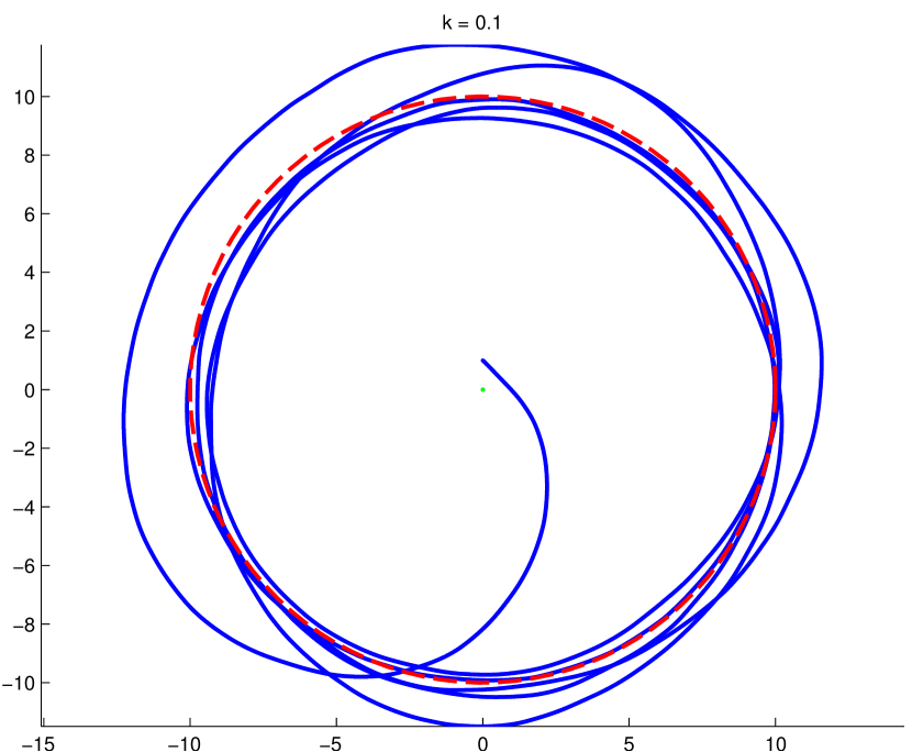
Figure 8: Trajectory with measurement error, $k=0.1$

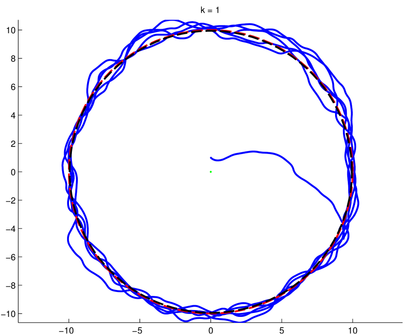
Figure 9: Trajectory with measurement error, $k=1$

Figure 9 shows the trajectory of the of UAV with gain size $k=0.1=r_{a}^{-1}$ corresponding to $r_{s}=0$, while Figure 9 shows the trajectory with gain size $k=1.0$ corresponding to $r_{s}=9.95$. We observe that the smaller gain size gives a smoother trajectory but larger deviations from the desired radius. The larger gain size adheres to the desired orbit more closely, but at the expense of a larger control effort.

We then run the simulation 20 times, increasing the gain $k$ on each iteration from the minimum value $k=0.1$ by increments of $0.15$, and collect statistics its performance. Figures 10 and 11 show the average of $(r-r_{a})^{2}$ and $\dot{r}^{2}$ respectively as the gain $k$ increases. This supports the observation from the trajectories that higher gain choices correspond to less radial error at the expense of smoothness and large control effort; though only to a point. If the maximum control adjustment $2kV$ is larger than $\pi$ (here corresponding when $k=\pi/2$), then the UAV may turn directly around instantaneously. Besides being quite impractical, this causes the UAV to over-correct and spin out of control.

Figure 10: Average mean-square error of $(r-r_{a})$

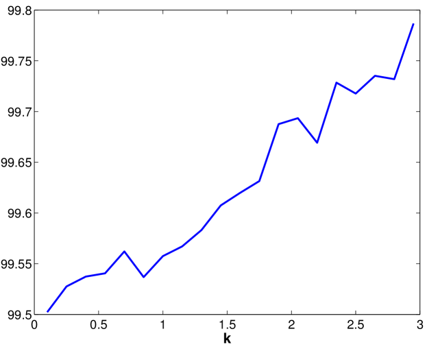
Figure 11: Average mean-square error of $\dot{r}$

V-B Measurement Error with Constant Wind

Here we examine the performance of the algorithm under the influence of measurement errors (as above) and constant wind. One may formulate the ‘windy’ system with constant wind bias of speed $W_{s}$ and direction $w_{d}$ as

$$\begin{aligned} d\left[\begin{array}[]{c}x\\ y\\ \psi\end{array}\right]=\left[\begin{array}[]{c}V\cos\psi+W_{s}\cos w_{d}\\ V\sin\psi+W_{s}\sin w_{d}\\ u\end{array}\right]dt+\left[\begin{array}[]{c}0\\ 0\\ -k\sigma\end{array}\right]d\xi.\end{aligned}$$ (24)

We simulate trajectories under such a wind model, using the same control policy $u$ as in (12). We take the windspeed $W_{s}=V/4=0.25$ and the wind direction $w_{d}=\pi/4$.

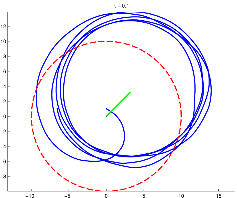
Figure 12: Trajectory with measurement error and wind, $k=0.1$

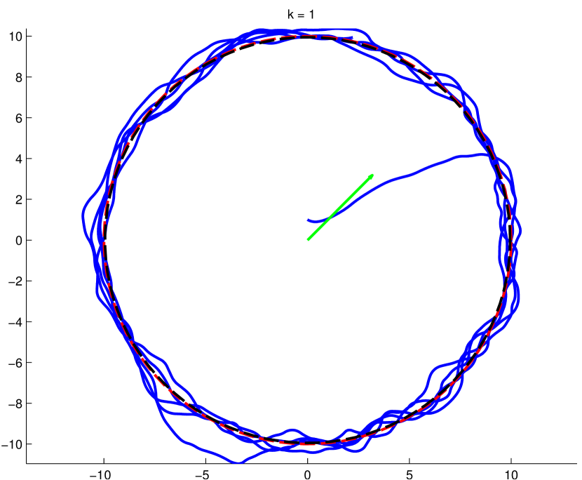
Figure 13: Trajectory with measurement error and wind, $k=1$

Figures 13 and 13 depict the windy trajectories analogous to the windy case. We note that with the minimal gain size the trajectory forms a circular orbit, but is shifted off-target in the direction of the wind. When the gain is turned up the UAV adjusts more dynamically and is able to adhere to the desired radius much better.

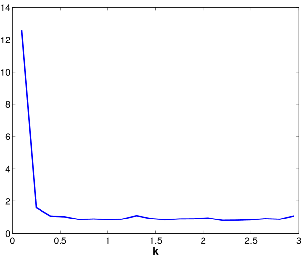
Figure 14: Average mean-square error of $(r-r_{a})$ with wind

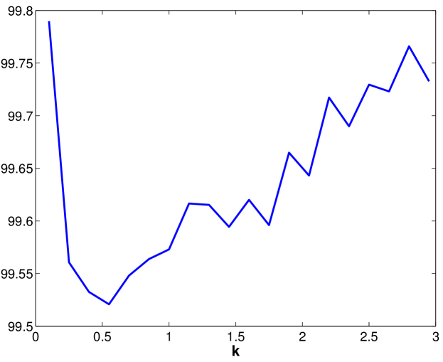
Figure 15: Average mean-square error of $\dot{r}$ with wind

Figures 14 and 15 show the mean-square error of $(r-r_{a})$ and $\dot{r}$ under the influence of wind and measurement errors.

VI Conclusion and Future Work

This paper has established a robust control policy for a UAV to circumnavigate a stationary target using noise-corrupted range and range rate measurements, without any use or assumption of location information for the UAV nor the target. Assuming additive measurement errors we established a recurrence result, bounding the time until the UAV reaches a neighborhood of the desired orbit, via a Lyapunov function approach. A simulation study was then used to collect statistics of the performance of the control policy with measurement errors, as well as with drifting bias due to the influence of wind.

Future work may attempt to establish that the trajectory is set-wise stable to the recurrent set, as simulations seem to suggest. Traditional stochastic stability results as in [7] are not applicable due to the persistence of noise (non-zero diffusion coefficient) at the ‘stability’ point $(r_{d},\pi/2)$. However, $p$th-moment set-wise stability in the sense of [9] may be possible.

Other research directions include formal analysis of the system with constant wind bias as in (24). The addition of wind terms in $\dot{x},\dot{y}$ prevent the reduction of the system to $(r,\theta)$. However, assuming one can additionally measure the heading angle $\psi$ (by addition of a magnometer), it is possible to formulate the current control and windy system dynamics in terms of $(r,\theta,\psi)$. Such conversion assumes $W_{s}$ and $w_{d}$ are known, but it may be possible to statistically estimate these quantities from a few revolutions of the target under the current control. For example, one sees in Figure 13 that with small gain there is significant bias of the orbit in direction of the wind. One may attempt to first estimate the wind direction $w_{d}$ as a statistical change-point problem from when the radius is under-biased to when it is over-biased. One may then try to estimate wind speed $W_{s}$ by the magnitude of such a change.

Finally, the addition of heading angle $\psi$ measurements may allow for other control schemes to be developed, perhaps resulting smoother trajectories and less control effort.

References

- [1] J. Gerler, ”U.S. Unmanned Aerial Systems”, Congressional Research Service Report, Jan. 2012. [Online]. Available: http://www.fas.org/sgp/crs/natsec/R42136.pdf
- [2] G. Warwick, Lightsquared tests confirm GPS jamming, Aviation Week, June 2011. [Online]. Available: http://www.aviationweek.com/aw/generic/story.jsp?id=news/awx/ 2011/06/09/awx06092011p0- 334122.xml
- [3] D. Shepard, J. Bhatti, and T. Humphreys, Drone hack: Spoofing attack demonstration on a civilian unmanned aerial vehicle, GPS World, 2012. [Online]. Available: http://www.gpsworld.com/drone-hack/
- [4] I. Shames, S. Dasgupta, B. Fidan, and B. D. O. Anderson, Circumnavigation Using Distance Measurements Under Slow Drift, IEEE Transactions on Automatic Control, vol. 57, no. 4, pp. 889 903, 2012.
- [5] M. Deghat, I. Shames, B. D. O. Anderson, and C. Yu, Target localization and circumnavigation using bearing measurements in 2D, in IEEE Transactions on Automatic Control, 2013.
- [6] Y. Cao, J. Muse, D. Casbeer, and D. Kingston, ”Circumnavigation of an Unknown Target Using UAVs with Range and Range Rate Measurements”, to appear in IEEE Conference on Decision and Control, 2013, available at arxiv.org/abs/1308.6250.
- [7] R. Khasminskii, Stochastic Stability of Differential Equations, Springer-Verlag, Berlin, 2011.
- [8] B. K. Øksendal, Stochastic Differential Equations: An Introduction with Applications, Springer-Verlag, Berlin, 2003.
- [9] D. Mateos-Núnẽz and J. Cortés, Stability of stochastic differential equations with additive persistent noise, in American Control Conference (ACC), 2013, 2013, pp. 5427 5432.