Exact, molecular-shaped vortices with fractional and integer charges in the extended Skyrme-Faddeev model

Abstract

We analytically construct vortex solutions in the integrable sector of the extended Skyrme-Faddeev model. The solutions are holomorphic type which satisfy the zero curvature condition. For the model parameter $\beta e^{2}=1$ there is a lump solution, and for $\beta e^{2}\neq 1$ new potentials are introduced for the several molecular-shaped solutions with half-integer or integer charges. They necessarily have infinite number of conserved currents and some of the examples are shown. By performing an annealing simulation with our potentials, we verify the existence of the solutions of the integrable sector.

I Introduction

The Skyrme-Faddeev model was introduced in the seventies sf as a clever generalization to $(3+1)$ dimensions of the $O(3)$ non-linear sigma model in $(2+1)$ dimensions bp . The Skyrme term, quartic in derivatives of the field, balances the quadratic kinetic term and according to Derrick’s theorem, allows the @existence of stable solutions with non-trivial Hopf topological charges. Due to the highly non-linear character of the model and the lack of symmetries, the first soliton solutions were only constructed in the late nineties using numerical methods Gladikowski:1996mb ; solfn ; sutcliffe ; hietarinta . Several physical applications based on the model have been extensively studied in many areas due mainly to the knotted character of the solutions babaev . The numerical efforts in the construction of the solutions have improved our understanding of the properties of the model improve and even the scattering of knotted solitons has been investigated hietarinta-scatter . One of the aspects of the model that has attracted considerable attention has been its connection with gauge theories. Faddeev and Niemi have conjectured that it might describe the low energy limit of the pure $SU(2)$ Yang-Mills theory fn . They based their argument on a decomposition of the physical degrees of freedom of the $SU(2)$ connection, proposed in the eighties by Cho chofn , and involving a triplet of scalar fields ${\vec{n}}$ taking values on the sphere $S^{2}$ (${\vec{n}}^{2}=1$). Gies gies has calculated the Wilsonian one loop effective action for the pure $SU(2)$ Yang-Mills theory assuming Cho’s decomposition, and found that the Skyrme-Faddeev action is indeed part of it, but additional quartic terms in the derivatives of the triplet ${\vec{n}}$ are unavoidable.

The extended version of such Skyrme-Faddeev (ESF) model,

$$\mathcal{L}=\mathcal{M}^{2}\partial_{\mu}\vec{n}\cdot\partial^{\mu}\vec{n}-\frac{1}{e^{2}}(\partial_{\mu}\vec{n}\wedge\partial_{\nu}\vec{n})^{2}$$

$$+\frac{\beta}{2}(\partial_{\mu}\vec{n}\cdot\partial^{\mu}\vec{n})^{2}-V(n_{1},n_{2},n_{3})$$ (1)

has already been studied: The static energy density (${\cal H}_{{\rm static}}=-{\cal L}$) associated to (1) is positive definite if $V>0$, $\mathcal{M}^{2}>0$, $e^{2}>0$ and $\beta<0$. That is the sector explored in Gladikowski:1996mb where Hopf soliton solutions were first constructed (for $V=0$). In addition, that is also the sector explored in Sawado:2005wa but with additional terms involving second derivatives of the ${\vec{n}}$ field, where Hopf solitons were also constructed. The static energy density of (1) is also positive definite for $V>0$ if

$$\mathcal{M}^{2}>0\,;\qquad e^{2}<0\,;\qquad\beta<0\,;\qquad\beta\,e^{2}\geq 1.$$ (2)

That is the sector that agrees with the signature of the terms in the one loop effective action calculated in gies and it is the sector that we will consider in this paper. Static Hopf solitons with the axial symmetry were constructed in Ferreira:2009gj ; Ferreira:2010zz for the sector (2) and their quantum excitations, including comparison with glue ball spectrum, were considered in quantumhopfions . An interesting feature of the Hopf solitons constructed in Ferreira:2009gj is that they shrink in size and then disappear as $\beta\,e^{2}\rightarrow 1$. Full numerical simulation was followed for the existence of such knotted solutions in Foster:2012wx .

The action (1) also possesses the vortex solutions. The first exact vortex solutions for the theory were constructed in vortexlaf , by exploring the integrability properties of a submodel of (1). In order to describe those exact vortex solutions, it is better to perform the stereographic projection of the target space $S^{2}$ onto the plane parameterized by the complex scalar field $u$ and related to ${\vec{n}}$ by

$${\vec{n}}=\left(u+u^{*},-i\left(u-u^{*}\right),\mid u\mid^{2}-1\right)/\left(1+\mid u\mid^{2}\right).$$ (3)

It was shown in vortexlaf that the field configurations of the form

$$u\equiv u\left(z,y\right),~{}~{}u^{*}\equiv u^{*}\left(z^{*},y\right)~{}~{}~{}~{}{\rm for}~{}~{}~{}~{}\beta\,e^{2}=1,~{}~{}V=0$$

are exact solutions of (1), where $z=x^{1}+i\,\varepsilon_{1}\,x^{2}$ and $y=x^{3}-\varepsilon_{2}\,x^{0}$, with $\varepsilon_{a}=\pm 1$, $a=1,2$ (the signs can be chosen independently). The $x^{\mu}$, $\mu=0,1,2,3$, are the Cartesian coordinates of the Minkowski space-time. Despite the fact that (LABEL:exactclass) constitutes a very large class of solutions, no finite energy solutions were found within it. If the dependence of the $u$ field upon the variable $y$ is in the form of phases like $e^{i\,k\,y}$, then one finds solutions with finite energy per unit of length along the $x^{3}$-axis. The simplest solution is of the form $u=z^{n}\,e^{i\,k\,y}$, with $n$ to be integer, and it corresponds to a vortex parallel to the $x^{3}$-axis and with waves travelling along it with the speed of light. More general solutions of the class (LABEL:exactclass) were constructed in newsf , including multi-vortices separated from each other and all parallel to the $x^{3}$-axis.

The vortex solutions for the model continue to exist when the condition $\beta e^{2}=1$ is relaxed by introducing a potential $V$ Ferreira:2011mz . The potential is essentially introduced to stabilize the vortex solutions. It is well known that there are some variations for the potential when it is a functional of the third component $n_{3}$ of the triplet ${\vec{n}}$, such as so-called old-baby potential (one-vacuum type; which has zero at the spatial infinity) Leese:1989gi and new-baby potential (two-vacuum type; which possesses two zeros at the origin and the infinity) Kudryavtsev:1997nw . The baby-Skyrme model is a 2+1 mimic of the Skyrme model and has the static planar solution called baby-skyrmions. The present model has close relation with the baby-Skyrme model when we restrict our analysis only in the static planar solution. In the old-baby potential, the rotational symmetry of the baby-skyrmions is spontaneously broken while in the new-baby, no such transition of the structure occurs Hen:2007in . Similar behavior has also been observed in our vortex solution Ferreira:2012cy . By using the old-baby potential, the deformation grows as $\beta e^{2}$ increases. Note that if the potential is a functional of the third component $n_{3}$ it breaks the $O(3)$ symmetry of the original Skyrme-Faddeev down to $O(2)$, the group of rotations on the plane $n_{1}-n_{2}$, and so eliminating two of the three Goldstone boson degrees of freedom.

If one allows to include all components $n_{1},n_{2}$ and $n_{3}$ in the potential, there must be many possibilities of the choice. In the easy plane potential $V=\frac{1}{2}m^{2}n_{3}^{2}$, the baby-skyrmions possess the dihedral symmetry $D_{2}$ Jaykka:2010bq . Originally, such a symmetrical solution was found by the choice of $V=\frac{1}{2}m^{2}(1-n_{3}^{2})(1-n_{1}^{2})$ Ward:2003xv . A sophisticated form of the potential $V=m^{2}|1-(n_{1}+in_{2})^{N}|^{2}(1-n_{3})~{}(N\geqq 2)$ is essentially the same as the old-baby but exhibits the $D_{N}$ symmetry Jaykka:2011ic . The baby-skyrmions or the fractional vortex states for a variant of these potentials are extensively investigated in Nitta . In general, one can get solutions with dihedral symmetries if one adopt potentials which contain terms with $n_{1}$ or (and) $n_{2}$ components. In most studies of this direction, the authors employ some potentials which are motivated by physics or mathematics, and they numerically solve the Euler-Lagrange equations or the Hamiltonian and get the desired solutions.

In Garaud:2012pn , the authors discussed a multi-band Ginzburg-Landau model. Especially, it forms several skyrmion exciations which exhibit molecular-like magnetic field configurations. The potential comprises of the standard Mexican hat and also the Josephson terms and the effects are thoroughly studied.

The method examined in Piette:1992he seems unique and independent from others. First the authors assume an existence of a static and exact $N-$centered solution. Next, they determine the form of the potential in order that the solution satisfies the Euler-Lagrange equation. They succeeded to get the analytical $N=2$ solution but failed to find $N>2$ ones and then the problem was solved only numerically. Although any guiding principle to find the solution and the potential is absent in their discussion, the idea seems promising. In this paper, we try to construct the exact $N-$centered vortex solutions and the corresponding potentials. First, we introduce the $N-$centered ansatz which is essentially similar with one proposed in Piette:1992he . Main difference is that our ansatz describes the time-dependent, travelling wave vortex solutions and these are exactly solution of the corresponding submodel equation. Plugging them into the Euler-Lagrange equation of the model and we are able to construct the potential in order that the solution of the submodel becomes one of the equations itself. As a result, we can get the analytical vortex solution of the model which possesses an infinite number of the conserved quantities. The method is straightforwardly applicable to the other related soliton models such as the baby-Skyrme model, the Skyrme model, so on.

The paper is organized as follows. In the next section we briefly describe the extended Skyrme-Faddeev model. The equations of motion are also introduced in Sec. II. The method how to get the solutions of the integrable sector of the present model is discussed in Sec. III. Sec.IV is devoted for the zero-curvature conditions and the conservation of the currents. In Sec V, we show the numerical solutions. A brief summary is presented in Sec. VI.

II The model

The Lagrangian density of the extended Skyrme Faddeev model reads (1), where unit vector $\vec{n}$, i.e. $\vec{n}\cdot\vec{n}=1$, is a triplet of real scalar fields taking values on the sphere $S^{2}$. The coupling constant $\mathcal{M}$ is dimensional whereas $e^{2}$ and $\beta$ are some dimensionless coupling constants. The potential $V$ depends on all the components of the triplet $\vec{n}$. One can introduce the complex fields $u$ and $u^{*}$ using a stereographic projection(3) which leads to the following expression for the Lagrangian

$$\mathcal{L}=4\mathcal{M}^{2}\frac{\partial_{\mu}u\partial^{\mu}u^{*}}{(1+|u|^{2})^{2}}+\frac{8}{e^{2}}\Big{[}\frac{(\partial_{\mu}u)^{2}(\partial_{\nu}u^{*})^{2}}{(1+|u|^{2})^{4}}$$

$$+(\beta e^{2}-1)\frac{(\partial_{\mu}u\partial^{\mu}u^{*})^{2}}{(1+|u|^{2})^{4}}\Big{]}-V(u,u^{*}).$$ (5)

If one set $\beta e^{2}=1$, then the model possesses some lump shaped analytical solutions in absence of the potential $V$. For the case of $\beta e^{2}\neq 1$, a potential is needed to stabilize the solution Ferreira:2011mz ; Ferreira:2010zz . In this paper, we try to find an exact form of potential for some solutions with $\beta e^{2}\neq 1$.
The Euler-Lagrange equations corresponding to (3) read

$$(1+|u|^{2})\partial^{\mu}\mathcal{K}_{\mu}-2u^{*}\mathcal{K}_{\mu}\partial^{\mu}u=-\frac{1}{4}(1+|u|^{2})^{3}\frac{\partial V}{\partial u^{*}},$$ (6)

together with the complex conjugated equation. The symbol $\mathcal{K}_{\mu}$ stands for the expression

$$\mathcal{K}_{\mu}\equiv\mathcal{M}^{2}\partial_{\mu}u+\frac{4}{e^{2}}\Bigl{[}\frac{(\partial_{\nu}u\partial^{\nu}u)\partial_{\mu}u^{*}}{(1+|u|^{2})^{2}}$$

$$+\frac{(\beta e^{2}-1)(\partial_{\nu}u\partial^{\nu}u^{*})\partial_{\mu}u}{(1+|u|^{2})^{2}}\Bigr{]}.$$ (7)

We use the dimensionless polar coordinates ($t$, $\rho$, $\varphi$, $z$) defined as follows

$$x_{0}=ct,~{}x_{1}=\rho\cos\varphi,~{}x_{2}=\rho\sin\varphi,~{}x_{3}=z.$$

Here we choose $c=1$. The metric is of the form

$$(ds)^{2}=\eta_{\mu\nu}dx^{\mu}dx^{\nu}=(dt)^{2}-(d\rho)^{2}-\rho^{2}(d\varphi)^{2}-(dz)^{2},$$

where

$$\eta_{\mu\nu}=\begin{pmatrix}1&0&0&0\\ 0&-1&0&0\\ 0&0&-\rho^{2}&0\\ 0&0&0&-1\\ \end{pmatrix},~{}~{}~{}~{}\det[\eta]=-\rho^{2}.$$

All classical configurations are characterised by the following topological charge

$$Q =\frac{1}{4\pi}\int\vec{n}\cdot(\partial_{\mu}\vec{n}\times\partial_{\nu}\vec{n})d^{2}x$$

$$=\frac{i}{2\pi}\int\frac{(\partial_{\rho}u\partial_{\varphi}u^{*}-\partial_{\varphi}u\partial_{\rho}u^{*})}{(1+|u|^{2})^{2}}\rho d\rho d\varphi.$$ (8)

This integer $Q$ is associated to the vortex, and defined as the winding number of the map from any circle on the $x$-$y$ plane centered at the $z$-axis.

III Construction of the exact solutions

III.1 The general formula

We would like to examine solutions which satisfy so called zero curvature condition Alvarez:1997ma . The zero curvature condition of the model reads

$$(\partial_{\mu}u)^{2}=0.$$ (9)

As we shall describe at Sec.IV in detail, the solution possesses an infinite set of conserved currents. Within the condition (9), the equation of motion (6) can be written as

$$\frac{\partial V}{\partial u^{*}}=\frac{1}{(1+|u|^{2})^{2}}\partial^{\mu}\biggl{[}\frac{16(\beta e^{2}-1)(\partial_{\nu}u\partial^{\nu}u^{*})\partial_{\mu}u}{e^{2}(1+|u|^{2})^{2}}\biggr{]}.$$ (10)

In order to find the explicit form of $V$, it is not straightforward, or not possible to solve the partial differential equation (10). In the following, we propose an ansatz to find a good candidate of $V$ which consists of a few steps:

• we construct a $N$-centered solution $u_{N}$ which satisfies the zero curvature condition (9),

• substituting the solution found in (i) into (10), we get the derivative of a potential

  $$\frac{\partial\bar{V}}{\partial u_{N}^{*}}$$

  $$=\frac{1}{(1+|u_{N}|^{2})^{2}}\partial^{\mu}\biggl{[}\frac{16(\beta e^{2}-1)(\partial_{\nu}u_{N}\partial^{\nu}u_{N}^{*})\partial_{\mu}u_{N}}{e^{2}(1+|u_{N}|^{2})^{2}}\biggr{]},$$

• we introduce a candidate of $V_{N}$ and examine its derivative $\dfrac{\partial V_{N}}{\partial u^{*}}$,

• we confirm that $V_{N}$ is correct by comparing $\dfrac{\partial V_{N}}{\partial u^{*}}$ and $\dfrac{\partial\bar{V}}{\partial u^{*}}$.

As a simple example, we consider a solution of the form

$$u_{N}=\frac{\rho e^{i\varphi}-\xi_{1}}{a}\frac{\rho e^{i\varphi}-\xi_{2}}{a}\frac{\rho e^{i\varphi}-\xi_{3}}{a}\cdots\frac{\rho e^{i\varphi}-\xi_{N}}{a}$$ (11)

where $\xi_{1},\xi_{2},\cdots,\xi_{N}(\in\mathbb{C})$ have a meaning of position of the center of each constituent, and $a$ is a scale parameter. For simplicity, we set the centers $\xi_{k}\equiv ce^{i(\alpha+\frac{2\pi(k-1)}{N})}$,where $k=1,\cdots,N$, and $\alpha$ and $c$ are arbitrary constants then the solution (11) is contracted in the form

$$u_{N}=\frac{1}{a^{N}}\left(\rho^{N}e^{iN\varphi}-\xi_{1}^{N}\right).$$ (12)

Substituting (12) into (10), we get

$$\frac{\partial\bar{V}}{\partial u_{N}^{*}}=-\frac{64N^{3}(\beta e^{2}-1)\Delta^{*1-\frac{2}{N}}\Delta^{2-\frac{2}{N}}}{a^{4}e^{2}\left(1+|u_{N}|^{2}\right)^{5}}\times$$

$$\biggl{[}1+|u_{N}|^{2}-N\biggl{\{}1-2\Bigl{(}\frac{\xi^{*}_{1}}{a}\Bigr{)}^{N}\biggl{(}\Delta-\Bigl{(}\frac{\xi_{1}}{a}\Bigr{)}^{N}\biggr{)}-|u_{N}|^{2}\biggr{\}}\biggr{]},$$ (13)

where $\Delta\equiv\Bigl{(}\dfrac{\rho}{a}\Bigr{)}^{N}e^{iN\varphi}$. We rewrite (13) by using

$$\Delta\to u_{N}+\left(\frac{\xi_{1}}{a}\right)^{N},~{}~{}\Delta^{*}\to u_{N}^{*}+\left(\frac{\xi^{*}_{1}}{a}\right)^{N}$$ (14)

and then

$$\dfrac{\partial\bar{V}}{\partial u_{N}^{*}}=\frac{-2\lambda}{N(1+|u_{N}|^{2})^{5}}$$

$$\times\biggl{[}\biggl{(}u_{N}+\Bigl{(}\frac{\xi_{1}}{a}\Bigr{)}^{N}\biggr{)}^{2-\frac{2}{N}}\biggl{(}u_{N}^{*}+\Bigl{(}\frac{\xi_{1}^{*}}{a}\Bigr{)}^{N}\biggr{)}^{1-\frac{2}{N}}$$

$$\times\biggl{\{}1+|u_{N}|^{2}-N\biggl{(}1-2\Bigl{(}\frac{\xi_{1}^{*}}{a}\Bigr{)}^{N}u_{N}-|u_{N}|^{2}\biggr{)}\biggr{\}}\biggr{]}$$ (15)

with

$$\lambda=\frac{-32N^{4}(\beta e^{2}-1)}{a^{4}e^{2}}.$$ (16)

Here a candidate of $V_{N}$ is introduced as

$$V_{N}=\frac{\lambda}{(1+|u_{N}|^{2})^{4}}\biggl{(}u_{N}+\Bigl{(}\frac{\xi_{1}}{a}\Bigr{)}^{N}\biggr{)}^{a}\biggl{(}u_{N}^{*}+\Bigl{(}\frac{\xi_{1}^{*}}{a}\Bigr{)}^{N}\biggr{)}^{b},$$ (17)

where $\lambda,a$ and $b$ are arbitrary constants. Comparing $\dfrac{\partial V_{N}}{\partial u^{*}}$ and $\dfrac{\partial\bar{V}}{\partial u^{*}}$, we can fix the constants and obtain the form of the potential

$$V_{N}=\frac{\lambda}{(1+|u_{N}|^{2})^{4}}\biggl{(}u_{N}+\Bigl{(}\frac{\xi_{1}}{a}\Bigr{)}^{N}\biggr{)}^{2-\frac{2}{N}}\biggl{(}u_{N}^{*}+\Bigl{(}\frac{\xi^{*}_{1}}{a}\Bigr{)}^{N}\biggr{)}^{2-\frac{2}{N}}.$$ (18)

In the next subsection, we consider the solutions with the several winding numbers (the centers) $N$ and the corresponding potentials.

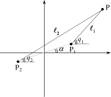
Figure 1: Schematic picture for the two-centered vortex solution. The each vortex sits on $(c,\alpha)$ and $(c,\alpha+\pi)$. Independently, they have the own radius and the azimuthal angle $(\ell_{i},q_{i}),~{}i=1,2$, which is used to describe the structure of each vortex.

III.2 Examples of the solutions and the corresponding potentials

For the construction of the solution and the potential, there have been already some studies based on the scheme Ferreira:2011mz ; Piette:1992he . First we present the results and then focus on several new multi-centered holomorphic solutions and the corresponding potentials.

III.2.1 The lump shaped solution and the corresponding potential

First we examine the case of the lump solution and see how the scheme works. The holomorphic vortex solution with the winding number $Q=1$ is vortexlaf

$$u_{1}=\Big{(}\frac{\rho}{a}\Big{)}e^{i[\varphi+k(t+z)]},$$ (19)

where $a$ is an arbitrary scale parameter. Note that it satisfies the zero curvature condition (9) and possesses an infinite set of the conserved quantities. It is easy to show that the following formulas hold

$$\partial_{\mu}u_{1}\partial^{\mu}u_{1}^{*}=-\frac{2}{\rho^{2}}|u_{1}|^{2},~{}~{}\partial^{\mu}\partial_{\mu}u_{1}=0.$$ (20)

Substituting (19) into (10), we get

$$\frac{\partial\bar{V}}{\partial u^{*}}\biggl{|}_{u=u_{1}}=-4\lambda\frac{u_{1}}{(1+|u_{1}|^{2})^{5}}.$$ (21)

On the other hand, plugging (19) into (18), we obtain

$$V_{1}=\lambda\frac{1}{(1+|u_{1}|^{2})^{4}}$$ (22)

and by taking derivative of this, we obtain

$$\frac{\partial V_{1}}{\partial u^{*}}\biggl{|}_{u=u_{1}}=-4\lambda\frac{u_{1}}{(1+|u_{1}|^{2})^{5}}.$$ (23)

(21) and $(\ref{pot_1center})$ are apparently equal and then (22) is valid in this case. In fact, it is the same as the one which was found in Ferreira:2011mz .

III.2.2 The two-centered solution and the potential

The solution with two-center can be written as a straightforward generalization of (19) such as

$$u_{2} =\Bigl{(}\frac{\ell_{1}}{a}\Bigr{)}\Bigl{(}\frac{\ell_{2}}{a}\Bigr{)}e^{i[(q_{1}+q_{2})+k(t+z)]}\,.$$ (24)

The solution possesses two “radii $\ell_{i}$” and “azimuthal angles $q_{i}$” with a scale parameter $a$, such that $\ell_{i}$ are a distances from a reference point $P$ and $q_{i}$ are angles measured from the horizontal axis. If we assume that each center is located at $(c,\alpha)$ and $(c,\alpha+\pi)$ in polar coordinate (Fig.1), $(\ell_{i},q_{i})$ are written in terms of the coordinate of $P$: $(\rho,\varphi)$ and $(c,\alpha)$ as

$$\ell_{1} :=\sqrt{\rho^{2}-2\rho c\cos(\varphi-\alpha)+c^{2}},$$

$$q_{1} :=\arctan\biggr{[}\frac{\rho\sin\varphi-c\sin\alpha}{\rho\cos\varphi-c\cos\alpha}\biggl{]};$$

$$\ell_{2} :=\sqrt{\rho^{2}+2\rho c\cos(\varphi-\alpha)+c^{2}},$$

$$q_{2} :=\arctan\biggr{[}\frac{\rho\sin\varphi+c\sin\alpha}{\rho\cos\varphi+c\cos\alpha}\biggl{]}.$$ (25)

After a bit lengthy calculation, we find form of the solution

$$u_{2}=\tilde{\rho}^{\hskip 3.0pt2}e^{i[2\varphi+k(t+z)]}-\tilde{c}^{\hskip 3.0pt2}e^{i[2\alpha+k(t+z)]},$$ (26)

where $\tilde{\rho}=\rho/a,\tilde{c}=c/a$. In the following, we omit ‘ $\tilde{~{}}$ ’ for simplicity. The static solution of (26),i.e., the case $k=0$, was already found as a static planar solution of the baby-Skyrme model Piette:1992he , in which the authors mainly focused on the effective force between the two constituents by using the solution. Of course (26) is also a solution of our model. It is easy to show that the following formulas hold

$$\partial_{\mu}u_{2}\partial^{\mu}u_{2}^{*}=-\frac{2}{\rho^{2}}|u_{2}|^{2},~{}~{}\partial^{\mu}\partial_{\mu}u_{2}=0.$$ (27)

Substituting (26) into (10), we get

$$\frac{\partial\bar{V}}{\partial u^{*}}\biggl{|}_{u=u_{2}}=-4\lambda\frac{(u_{2}+c^{2})(-1+3|u_{2}|^{2}+4c^{2}u_{2})}{(1+|u_{2}|^{2})^{5}}.$$ (28)

On the other hand, substituting (26) into (18), we obtain

$$V_{2}=\lambda\frac{(u_{2}+c^{2})(u_{2}^{*}+c^{2})}{(1+|u_{2}|^{2})^{4}}$$ (29)

and the derivative

$$\frac{\partial V_{2}}{\partial u^{*}}\biggl{|}_{u=u_{2}}=-4\lambda\frac{(u_{2}+c^{2})(-1+3|u_{2}|^{2}+4c^{2}u_{2})}{(1+|u_{2}|^{2})^{5}}.$$ (30)

Since (28) and (30) coincide then (29) is valid. In terms of the $\vec{n}$ field, the potential has the form

$$V_{2}=\frac{\lambda}{16}\Big{\{}n_{1}+in_{2}+c^{2}e^{i[2\alpha+k(t+z)]}(1-n_{3})\Big{\}}$$

$$\times\Big{\{}n_{1}-in_{2}+c^{2}e^{-i[2\alpha+k(t+z)]}(1-n_{3})\Big{\}}(1-n_{3})^{2}$$ (31)

which coincides with the static case $k=0$ in Piette:1992he .

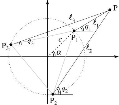
Figure 2: Schematic picture for the three-centered vortex solution. The each vortex sits on $(c,\alpha),(c,\alpha+\frac{2}{3}\pi),(c,\alpha+\frac{4}{3}\pi)$, respectively. Almost independently, they have the own radius and the azimuthal angle $(\ell_{i},q_{i}),~{}i=1,2,3$, which is used to describe the structure of the vortex.

III.2.3 The three-centered solution

We would like to apply the scheme for more complex systems. The first non-trivial case is with the three-center. Construction of a holomorphic solution with three isolated centers is not straightforward and a geometrical understanding is helpful. In Fig.2, we schematically draw a picture about the location of the core of vortices and the coordinates. As before we define a reference point $P$ which has a component $(\rho,\varphi)$ of a two dimensional polar coordinate. We consider the case that the vortices sit on the three tops of an equilateral triangle. The tops of the triangle $P_{i},i=1,2,3$ are located on a circle with the radius $c$. If $P_{1}$ has a component $(c,\alpha)$ in the polar coordinate, the remaining $P_{2},P_{3}$ are then $(c,\alpha+\frac{2}{3}\pi),(c,\alpha+\frac{4}{3}\pi)$, respectively. In order to construct the solution, according to the case of $n=1$ (19) we introduce “the radius $\ell_{i}$” and “the azimuthal angle $q_{i}$” of $P_{i}$, such that $\ell_{i}$ are distances between $P$ and $P_{i}$. $q_{i}$ are angles measured from the horizontal axis. The solution with three-center is described in terms of these coordinates such as

$$u_{3} =\Bigl{(}\frac{\ell_{1}}{a}\Bigr{)}\Bigl{(}\frac{\ell_{2}}{a}\Bigr{)}\Bigl{(}\frac{\ell_{3}}{a}\Bigr{)}e^{i[(q_{1}+q_{2}+q_{3})+k(t+z)]}.$$ (32)

The relation between the $(\ell_{i},q_{i})$ and the polar coordinate $(\rho,\varphi)$, $(c,\alpha)$ are

$$\ell_{1} :=\sqrt{\rho^{2}-2\rho c\cos(\varphi-\alpha)+c^{2}},$$

$$q_{1} :=\arctan\biggr{[}\frac{\rho\sin\varphi-c\sin\alpha}{\rho\cos\varphi-c\cos\alpha}\biggl{]};$$

$$\ell_{2} :=\sqrt{\rho^{2}+\rho c\cos(\varphi-\alpha)-\sqrt{3}\rho c\sin(\varphi-\alpha)+c^{2}},$$

$$q_{2} :=\arctan\biggr{[}\frac{2\rho\sin\varphi-\sqrt{3}c\cos\alpha+c\sin\alpha}{2\rho\cos\varphi+c\cos\alpha+\sqrt{3}c\sin\alpha}\biggl{]};$$

$$\ell_{3} :=\sqrt{\rho^{2}+\rho c\cos(\varphi-\alpha)+\sqrt{3}\rho c\sin(\varphi-\alpha)+c^{2}},$$

$$q_{3} :=\arctan\biggr{[}\frac{2\rho\sin\varphi+\sqrt{3}c\cos\alpha+c\sin\alpha}{2\rho\cos\varphi+c\cos\alpha-\sqrt{3}c\sin\alpha}\biggl{]}.$$ (33)

Finally, we write down the form of the solution as

$$u_{3}=\rho^{3}e^{i[3\varphi+k(t+z)]}-c^{3}e^{i[3\alpha+k(t+z)]}.$$ (34)

Note that the solution (34) is holomorphic and then, it satisfies the zero curvature condition (9)

$$(\partial_{\mu}u_{3})^{2} =\eta^{\mu\nu}\partial_{\mu}u_{3}\partial_{\nu}u_{3}$$

$$=(\partial_{t}u_{3})^{2}-(\partial_{\rho}u_{3})^{2}-\frac{1}{\rho^{2}}(\partial_{\varphi}u_{3})^{2}-(\partial_{z}u_{3})^{2}$$

$$=(iku_{3})^{2}-\Bigl{(}\frac{3}{\rho}\psi\Bigr{)}^{2}-\frac{1}{\rho^{2}}(3i\psi)^{2}-(iku_{3})^{2}$$

$$=0,$$ (35)

where $\psi\equiv\rho^{\hskip 3.0pt3}e^{3i\varphi}e^{ik(t+z)}$. Substituting (34) into (10), we find the potential

$$V_{3} =\frac{\lambda}{16}\Big{\{}n_{1}+in_{2}+c^{3}e^{i[3\alpha+k(t+z)]}(1-n_{3})\Big{\}}^{\frac{4}{3}}$$

$$\times\Big{\{}n_{1}-in_{2}+c^{3}e^{-i[3\alpha+k(t+z)]}(1-n_{3})\Big{\}}^{\frac{4}{3}}(1-n_{3})^{\frac{4}{3}}.$$ (36)

III.2.4 The $N$-centered solution

The generalization is now almost straightforward. We assume the center of the vortices sit on the $N$-th tops of a equilateral polygon and the $N$-centered solution should be written as

$$u_{N}=\rho^{N}e^{i[N\varphi+k(t+z)]}-c^{N}e^{i[N\alpha+k(t+z)]}.$$ (37)

The solution (37) still satisfies the zero curvature condition (9) and then has an infinite number of conserved quantities. We get the following form of the potential for $N$-centered solution

$$V_{N}=\frac{\lambda}{16}\Big{\{}n_{1}+in_{2}+c^{N}e^{i[N\alpha+k(t+z)]}(1-n_{3})\Big{\}}^{2-\frac{2}{N}}$$

$$\hskip 28.45274pt\times\Big{\{}n_{1}-in_{2}+c^{N}e^{-i[N\alpha+k(t+z)]}(1-n_{3})\Big{\}}^{2-\frac{2}{N}}$$

$$\hskip 142.26378pt\times(1-n_{3})^{\frac{4}{N}}.$$ (38)

For the special case such as $c=0$ the potential (38) becomes $V_{N}\to(1+n_{3})^{2-2/N}(1-n_{3})^{2+2/N}$, which perfectly agree with the result that we previously found in Ferreira:2011mz .

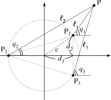
Figure 3: Schematic picture for the isosceles triangle vortex solution. Independently, they have the own radius and the azimuthal angle $(\ell_{i},q_{i}),~{}i=1,2,3$, which is used to describe the structure of the vortex.

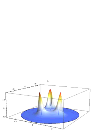
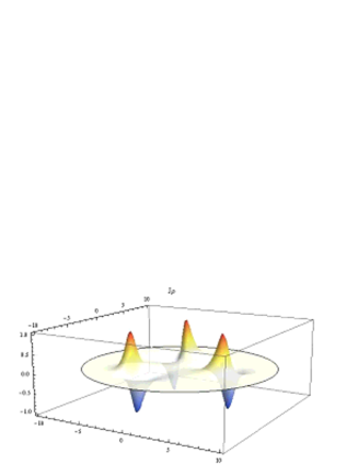
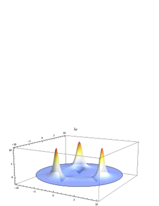
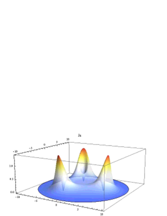
Figure 4: An U(1) current with the components $J_{t}$ (top left), $J_{\rho}$ (top right), $J_{\varphi}$ (bottom left) and $J_{z}$ (bottom right) (in unit of $-1/8{\cal M}^{2}$) with $N=3$ for $\beta=-2.0,e^{2}=-1.0,k=0.0$ and $c=1.0$.

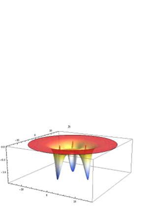
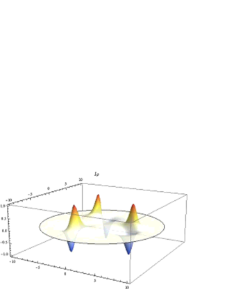
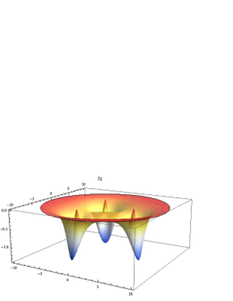
Figure 5: The components of a current which is defined by (54): $J_{t}$ (top left), $J_{\rho}$ (top right), $J_{\varphi}$ (bottom left) and $J_{z}$ (bottom right) (in unit of $-1/8{\cal M}^{2}$) with $N=3$ for $\beta=-2.0,e^{2}=-1.0,k=0.0$ and $c=1.0$.

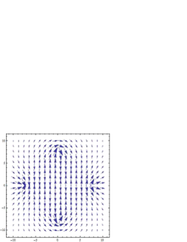
Figure 6: The arrow plot $(n_{1},n_{2})$ corresponding to the solution (43) of the $Q=2$ (top), $3$ (bottom) with $\beta e^{2}=2.0$, $k=0.0$ and $c=2.0$.

III.2.5 The isosceles triangle

Is it possible to give further generalization of the scheme of the construction such as an isosceles triangle for $N=3$? The schematic picture is shown in Fig. 3. Here the centers sit $(d_{1},d_{2}),(d_{1},-d_{2})$ and $(-c,0)$ in the cartessian coordinate. The relation between the $(\ell_{i},q_{i})$, the polar coordinate $(\rho,\varphi)$ and $(d_{1},d_{2})$ are

$$\ell_{1} :=\sqrt{c^{2}+2c\rho\cos\varphi+\rho^{2}},$$

$$q_{1} :=\arctan\biggr{[}\frac{\rho\sin\varphi}{c+\rho\cos\varphi}\biggr{]};$$

$$\ell_{2} :=\sqrt{(\rho\cos\varphi-d_{1})^{2}+(\rho\sin\varphi-d_{2})^{2}},$$

$$q_{2} :=\arctan\biggr{[}\frac{\rho\sin\varphi-d_{2}}{\rho\cos\varphi-d_{2}}\biggr{]};$$

$$\ell_{3} :=\sqrt{(\rho\cos\varphi-d_{1})^{2}+(\rho\sin\varphi+d_{2})^{2}},$$

$$q_{3} :=\arctan\biggr{[}\frac{\rho\sin\varphi+d_{2}}{\rho\cos\varphi-d_{2}}\biggr{]}.$$ (39)

Finally, we write down the form of the solution as

$$u =\Bigl{(}\frac{\ell_{1}}{a}\Bigr{)}\Bigl{(}\frac{\ell_{2}}{a}\Bigr{)}\Bigl{(}\frac{\ell_{3}}{a}\Bigr{)}e^{i[(q_{1}+q_{2}+q_{3})+k(t+z)]}$$

$$=\left(\rho e^{i\varphi}+c\right)\left(\left(\rho e^{i\varphi}-\tilde{d_{1}}\right)^{2}+\tilde{d_{2}}^{\hskip 3.0pt2}\right),$$ (40)

where $\tilde{d_{1}}=d_{1}/a,\tilde{d_{2}}=d_{2}/a$. Again we omit ‘ $\tilde{~{}}$ ’ . Note that the solution (40) is holomorphic and then, it satisfies the zero curvature condition (9). Substituting (40) into (10) and a guess of suitable form of the potential, the form is determined such as

$$V_{\tilde{3}}= -\frac{16\left(\beta e^{2}-1\right)}{e^{2}\left(1+(\mathcal{A}+c)(\mathcal{A}^{*}+c)\mathcal{B}\right)^{4}}$$

$$\times\left((d_{1}-\mathcal{A})(d_{1}-3\mathcal{A}-2c)+d_{2}^{2}\right)^{2}$$

$$\times\left((d_{1}-\mathcal{A}^{*})(d_{1}-3\mathcal{A}^{*}-2c)+d_{2}^{2}\right)^{2},$$ (41)

where $\mathcal{A}$ and $\mathcal{B}$ are defined as

$$\mathcal{A}=\frac{1}{3}(2d_{1}-c),$$

$$+\frac{\left(\sqrt{\zeta^{2}+4\tau^{3}}+\zeta\right)^{\frac{1}{3}}}{3\sqrt[3]{2}}-\frac{\sqrt[3]{2}\tau}{3\left(\sqrt{\zeta^{2}+4\tau^{3}}+\zeta\right)^{\frac{1}{3}}},$$

$$\mathcal{B}=\left((d_{1}-\mathcal{A})^{2}+d_{2}^{2}\right)\left((d_{1}-\mathcal{A}^{*})^{2}+d_{2}^{2}\right),$$

$$\zeta=27u-18d_{2}^{2}(c+d_{1})-2(c+d_{1})^{3},$$

$$\tau=3d_{2}^{2}-(c+d_{1})^{2}.$$ (42)

In the special choice $d_{1}=\frac{c}{2}$, the potential (41) perfectly agrees with (36).

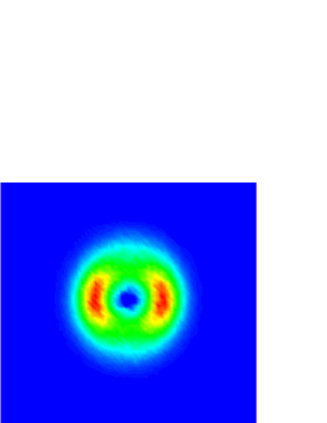
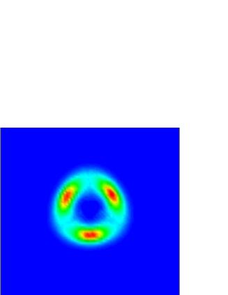
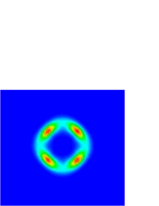
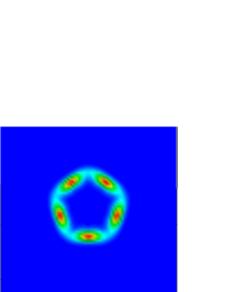
Figure 7: The hamiltonian densities of the $Q=2,3,4,5$ for $\beta=-2.0,e^{2}=-1.0,k=0.0$ and $c=1.0$.

III.2.6 The half-integer charged vortex solution and the potential

In Nitta , a fractional vortex polygons are studied in terms of a simple potential $V=n_{3}^{2}$ which is inspired in antiferromagnets and the $XY$ model. Our scheme can apply for construction of the half-integer charged vortex solution and the corresponding potential. The solution can be written as an extension of (37)

$$u=\sqrt{\rho^{\hskip 3.0ptN}e^{i[N\varphi+k(t+z)]}-c^{\hskip 3.0ptN}e^{i[N\alpha+k(t+z)]}}.$$ (43)

It is almost straightforward to check that (43) satisfies the zero curvature condition (9).

Substituting (43) into (8), one can see that the topological charge $Q=\frac{N}{2}$. Then, (43) comprises the $N-$centered solution in which a each constituent carries half integer fraction of the charge. In order to see the structure in more detail, we present the arrow plot of $(n_{1},n_{2})$ for $Q=2,3$. One can easily see that the solutions exhibit a half of winding with each vortex core. Substituting (43) into (10), we have the potential of the form

$$V_{\frac{N}{2}}= \frac{\lambda}{256}\Big{\{}\left(n_{1}+in_{2}\right)^{2}+c^{\hskip 3.0ptN}e^{i[N\alpha+k(t+z)]}(1-n_{3})^{2}\Big{\}}^{2-\frac{2}{N}}$$

$$\times\Big{\{}\left(n_{1}-in_{2}\right)^{2}+c^{\hskip 3.0ptN}e^{-i[N\alpha+k(t+z)]}(1-n_{3})^{2}\Big{\}}^{2-\frac{2}{N}}$$

$$\hskip 142.26378pt\times\frac{(1-n_{3})^{\frac{8}{N}}}{(1-n_{3}^{2})^{2}}.$$ (44)

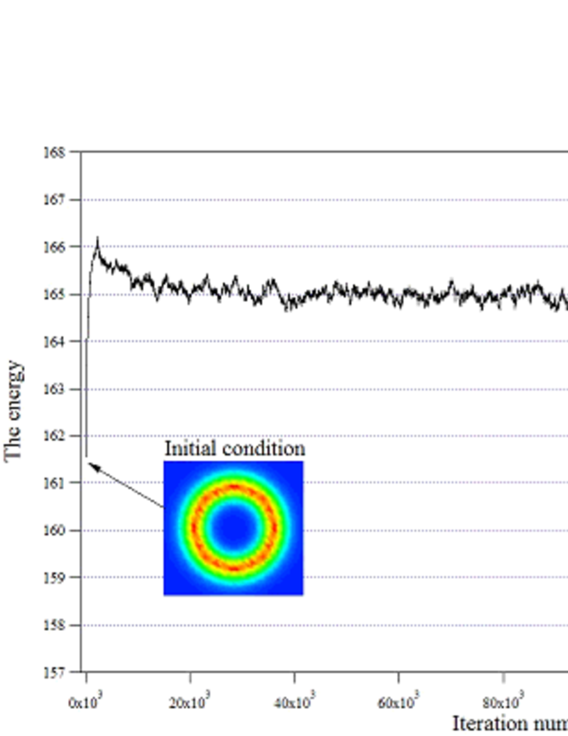
Figure 8: Energy per charge for the simulation of the $Q=3$ with $\beta e^{2}=2.0,e^{2}=-1.0,k=0.0$ and $c=1.0$.

IV The zero curvature condition

The potentials that we found in the previous section may be obtained in a slightly different way. Substituting the solution (37) into the potential (18), we get

$$V_{N}\to\frac{-32N^{4}(\beta e^{2}-1)\rho^{4N-4}}{a^{4N}\left(1+|u|^{2}\right)^{4}}.$$ (45)

On the other hand, substituting the solution (37) into the second term of order four in derivatives of the fields of the lagrangian (5), we get

$$\frac{(\beta e^{2}-1)(\partial_{\mu}u\partial^{\mu}u^{*})^{2}}{(1+|u|^{2})^{4}}\to\frac{4N^{4}(\beta e^{2}-1)\rho^{4N-4}}{a^{4N}\left(1+|u|^{2}\right)^{4}}.$$ (46)

Apparently this means that at least on the holomorphic solutions, the potential is identified to the term of order four in derivatives of the fields up to some constants. Thus we expect that when the solution is the holomorphic ones, the potential (18) can always be rewritten as

$$V_{N}\to-8\frac{(\beta e^{2}-1)(\partial_{\mu}u\partial^{\mu}u^{*})^{2}}{(1+|u|^{2})^{4}}.$$ (47)

By our zero curvature solutions, the term in the denominator of (47) generally can be calculated such as $\partial_{\mu}u\partial^{\mu}u^{*}=F(u,u^{*})$, where the $F(u,u^{*})$ is a function depends only on $u$ and $u^{*}$ (not on the derivatives). If one plugs the explicit form of $F(u,u^{*})$ into (47), one can obtain all potentials found in the previous subsections. Also, from (47) the potential is essentially equivalent to the term of order four in derivatives of the fields, and it is straightforward to see that the current is conserved in terms of the equivalence.

The zero curvature condition was first proposed in the context of the $CP^{1}$ model for integrable theories in any dimension Alvarez:1997ma , and then applied to many models with target space being the sphere $S_{2}$, or $CP^{N}$ Alvarez:2009dt . It leads to an infinite number of local conserved currents. Indeed, the equation of motion (6) implies the conserved currents given by

$$J^{G}_{\mu}\equiv\tilde{\mathcal{K}}_{\mu}\frac{\delta G}{\delta u}-\tilde{\mathcal{K}}^{*}_{\mu}\frac{\delta G}{\delta u^{*}},$$ (48)

where $G$ is assumed to be any functional of $u,u^{*}$. $\tilde{\mathcal{K}}_{\mu}$ can be defined as follows

$$\tilde{\mathcal{K}}_{\mu}=\mathcal{M}^{2}\partial_{\mu}u+\frac{4}{e^{2}}\biggl{[}\frac{(\partial_{\nu}u\partial^{\nu}u)\partial_{\mu}u^{*}}{(1+|u|^{2})^{2}}$$

$$\hskip 14.22636pt+\frac{2(\beta e^{2}-1)(\partial_{\nu}u\partial^{\nu}u^{*})\partial_{\mu}u}{(1+|u|^{2})^{2}}\biggr{]}$$ (49)

in terms of the equivalence (47).

The current is conserved because in the derivative of the current

$$\partial^{\mu}J^{G}_{\mu} =\frac{\delta^{2}G}{\delta u^{2}}\partial^{\mu}u\tilde{\mathcal{K}}_{\mu}+\frac{\delta G}{\delta u}\partial^{\mu}\tilde{\mathcal{K}}_{\mu}+\frac{\delta^{2}G}{\delta u\delta u^{*}}\partial^{\mu}u^{*}\tilde{\mathcal{K}}_{\mu}$$

$$-\frac{\delta^{2}G}{\delta u^{*2}}\partial^{\mu}u^{*}\tilde{\mathcal{K}}^{*}_{\mu}-\frac{\delta G}{\delta u^{*}}\partial^{\mu}\tilde{\mathcal{K}}^{*}_{\mu}-\frac{\delta^{2}G}{\delta u^{*}\delta u}\partial^{\mu}u\tilde{\mathcal{K}}^{*}_{\mu}.$$ (50)

The first and fourth term vanish due to the constraint (9), and the third and sixth term cancel out, and the second and fifth term vanish because now the Euler-Lagrange equation has the form

$$\partial^{\mu}\tilde{\mathcal{K}}_{\mu}=0,~{}~{}\partial^{\mu}\tilde{\mathcal{K}}_{\mu}^{*}=0.$$ (51)

Thus the current $J^{G}_{\mu}$ is conserved and leads to an infinite number of conserved quantities. If we choose the functional as

$$G:=-\frac{4i}{1+|u|^{2}},$$ (52)

one gets the corresponding conserved current

$$J_{\mu}|_{U(1)}= -4iM^{2}\frac{u\partial_{\mu}u^{*}-u^{*}\partial_{\mu}u}{(1+|u|^{2})^{2}}$$ (53)

$$-i\frac{8(\beta e^{2}-1)}{e^{2}}\frac{2(\partial_{\nu}u\partial^{\nu}u^{*})(\partial_{\mu}u^{*}u-u^{*}\partial_{\mu}u)}{(1+|u|^{2})^{4}}$$

which corresponds to the Noether current for the (1) associated to the symmetry $u\to ue^{i\alpha}$. In Fig. 4, we plot the components $J_{t},J_{\rho},J_{\varphi},J_{z}$ of the current for $N=3$. Of course we are able to compute the current corresponding to the other symmetries. As an example, we plot a current in terms of

$$G:=-\frac{4i|u|^{2}}{1+|u|^{2}}$$ (54)

in Fig. 5.

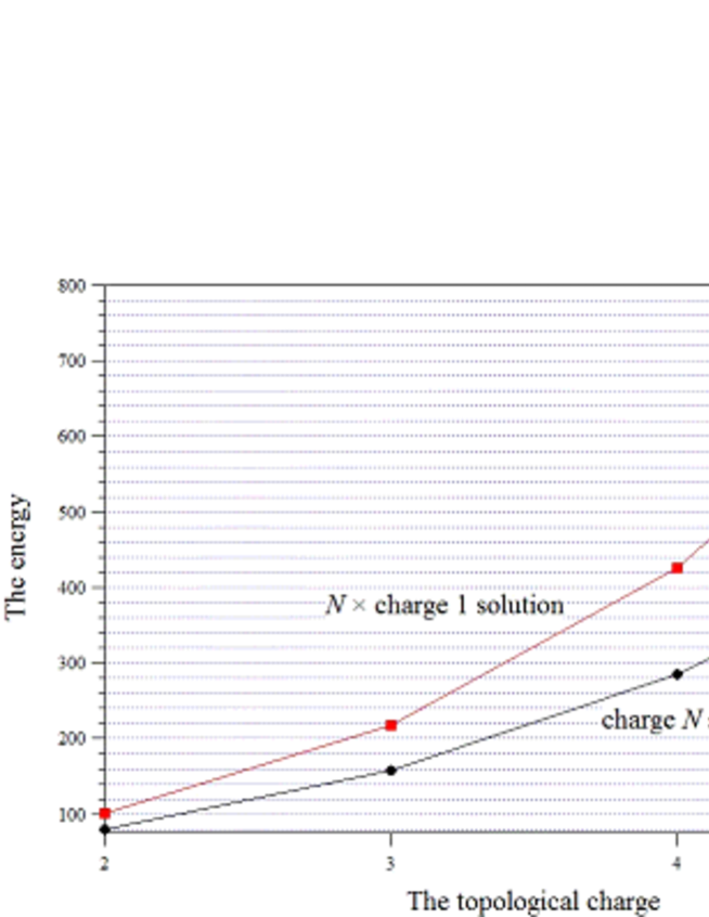
Figure 9: Energies of the solutions $Q=N=2,3,4,5$ and the ($N$ times of) the charge 1 solution with $\beta e^{2}=2.0,e^{2}=-1.0,k=0.0$, and $c=1.0$.

V The numerical study

Assuming the form of the solutions which satisfy the zero curvature condition, we have obtained the potentials (38) for general $N$. It seems not straightforward that the converse is also true, i.e., such potentials can produce solutions which we initially assumed. It is not easy question to answer and we solve the problem numerically. The simulated annealing method Hale:2000fk is a Hamiltonian minimization scheme which successfully finds the solution without any assumption for the solution. However, in order to get solutions with infinite number of conserved quantities, a few conditions are applied to our numerical analysis. First, we assume the solution can be decomposed such as

$$u={\cal U}(x,y){\cal W}(z,t)$$ (55)

where ${\cal U},{\cal W}\in\mathbb{C}$. Second, we explore the solution traveling along $z$ axis with speed of light, which is consistent with our analytical solutions. If ${\cal W}$ is a function of the light-cone coordinate, i.e., ${\cal W}(z,t)\equiv W(z\pm t)$, one can easily see that the lagrangian (5) except for the potential term becomes static. In general, the potential still has some time dependence. It also becomes static when we consider the case

$${\cal W}(z,t)\equiv e^{ik(z\pm t)}.$$ (56)

In order to get solutions with infinite number of conserved quantities, the crucial point is that the potential can be rewritten as one of the term of order four in derivatives of the field as we discussed in the last section. Thus, if the fourth order term is static, the potential should also be time independent. This clearly indicates that the ansatz (55) and (56) are valid for finding solutions with infinite number of conserved quantities. As a result, we explore solution by minimizing the static Hamiltonian based on the ansatz (55) and (56). Of course, we admit that outside these conditions there might be some solutions which still satisfy the zero curvature condition, but finding such solutions is obviously challenging but has to be quite difficult task. Thus we concentrate on analysis based on our assumption. If one evaluates the Hamiltonian density $\cal H$ for the Lagrangian (5) and then imposes the conditions (55) and (56) one obtains

$${\cal H}= \frac{4{\mathcal{M}}^{2}}{(1+|{\cal U}|^{2})^{2}}(2k^{2}|{\cal U}|^{2}+\partial_{x}{\cal U}\partial_{x}{\cal U}^{*}+\partial_{y}{\cal U}\partial_{y}{\cal U}^{*})$$

$$+\frac{8}{e^{2}(1+|{\cal U}|^{2})^{4}}\big{\{}\big{(}(\partial_{x}{\cal U})^{2}+(\partial_{y}{\cal U})^{2}\big{)}$$

$$\times\big{(}(\partial_{x}{\cal U}^{*})^{2}+(\partial_{y}{\cal U}^{*})^{2}\big{)}-2k^{2}{\cal U}^{2}\big{(}(\partial_{x}{\cal U}^{*})^{2}+(\partial_{y}{\cal U}^{*})^{2}\big{)}$$

$$-2k^{2}{\cal U}^{*2}\big{(}(\partial_{x}{\cal U})^{2}+(\partial_{y}{\cal U})^{2}\big{)}\big{\}}$$

$$+\frac{8(\beta e^{2}-1)}{e^{2}(1+|{\cal U}|^{2})^{4}}\big{\{}(\partial_{x}{\cal U}\partial_{x}{\cal U}^{*}+\partial_{y}{\cal U}\partial_{y}{\cal U}^{*})$$

$$\times\big{(}4k^{2}|{\cal U}|^{2}+(\partial_{x}{\cal U}\partial_{x}{\cal U}^{*}+\partial_{y}{\cal U}\partial_{y}{\cal U}^{*})\big{)}\big{\}}.$$ (57)

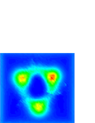
Figure 10: The hamiltonian density of the isosceles triangle of the $Q=3$ with $\beta=-2.0,e^{2}=-1.0,k=0.0$ and $c=3.0$.

Figure 11: The hamiltonian density of the half vortex of the $Q=2$ (left), 3 (right) with $\beta=-2.0,e^{2}=-1.0,k=0.0$ and $c=1.0$.

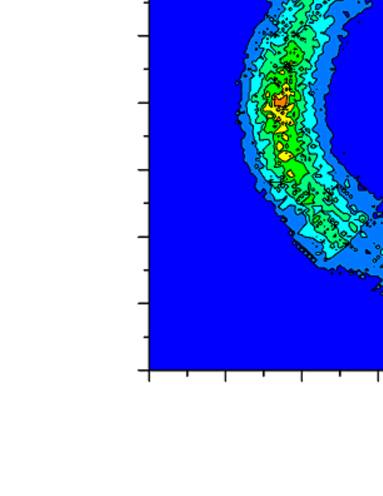
Figure 12: The zero curvature condition in terms of the annealing simulation, of the $Q=3$ with $\beta e^{2}=2.0,e^{2}=-1.0$, $k=0.0$ and $c=1.0$.

For ${\cal U}$, without loss of generality we can parameterize ${\cal U}:=F(x,y)e^{i\Theta(x,y)}$. However, for the numerical simulation it is more convenient to use a static field $\vec{m}$ than ${\cal U}$ which has of the form

$$\vec{m} = \left({\cal U}+{\cal U}^{*},-i({\cal U}-{\cal U}^{*}),|{\cal U}|^{2}-1\right)/\left(1+|{\cal U}|^{2}\right)$$ (58)

$$= \left(\sin f\cos\Theta,\sin f\sin\Theta,\cos f\right),$$

where $\sin f(x,y):=\frac{2F(x,y)}{1+F(x,y)^{2}},\cos f(x,y):=\frac{F(x,y)^{2}-1}{1+F(x,y)^{2}}$.

Substituting (58) into (57) we have a form of static Hamiltonian density

$${\cal H}_{xy}=\mathcal{M}^{2}\{{\cal P}_{x}+{\cal P}_{y}+2k^{2}(1+\cos^{2}f)\}$$

$$\hskip 14.22636pt-\frac{1}{2e^{2}}\bigg{\{}{\cal P}_{x}^{2}+{\cal P}_{y}^{2}+2(f_{x}f_{y}+\sin^{2}f\Theta_{x}\Theta_{y})^{2}$$

$$\hskip 28.45274pt+2\sin^{2}f(f_{x}\Theta_{y}-f_{y}\Theta_{x})^{2}-2k^{2}\sin^{2}f({\cal Q}_{x}+{\cal Q}_{y})\bigg{\}}$$

$$\hskip 14.22636pt-\frac{\beta e^{2}-1}{2e^{2}}({\cal P}_{x}+{\cal P}_{y})\big{(}{\cal P}_{x}+{\cal P}_{y}+4k^{2}\sin^{2}f\big{)}$$

$$\hskip 14.22636pt+V$$ (59)

where

$${\cal P}_{x,y}:=f_{x,y}^{2}+\sin^{2}f\Theta_{x,y}^{2},~{}{\cal Q}_{x,y}:=f_{x,y}^{2}-\sin^{2}f\Theta_{x,y}^{2}$$ (60)

with $f_{x}=\frac{\partial f}{\partial x},f_{y}=\frac{\partial f}{\partial y},\Theta_{x}=\frac{\partial\Theta}{\partial x}$, and $\Theta_{x}=\frac{\partial\Theta}{\partial y}$. We numerically minimize the static energy ${\cal H}_{xy}|_{k=0}$. The static potential, e.g., the case of the standard integer $N$, can be written as

$$V_{N} =\frac{\lambda}{16}\Big{\{}\sin{f}e^{i\Theta}+c^{\hskip 3.0ptN}e^{iN\alpha}(1-\cos{f})\Big{\}}^{2-\frac{2}{N}}$$

$$\hskip 28.45274pt\times\Big{\{}\sin{f}e^{-i\Theta}+c^{\hskip 3.0ptN}e^{-iN\alpha}(1-\cos{f})\Big{\}}^{2-\frac{2}{N}}$$

$$\hskip 28.45274pt\times(1-\cos{f})^{\frac{4}{N}}.$$ (61)

The simulated annealing is a Monte-Carlo simulation in which one improve the value of the fields $\vec{m}$ (or equivalently $f$ and $\Theta$) by using a random numbers so as reducing the energy. However, a more sophisticated method should be applied to the present problem. The method is the application of the Metropolis algorithm which can successfully avoids the unwanted saddle points.

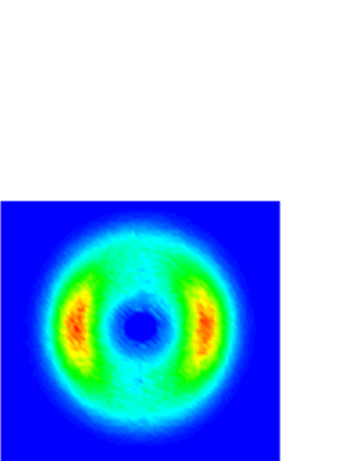
Figure 13: The hamiltonian densities with $k=0$ (left), $0.02$ (right) of the $Q=2$ with $\beta=-2.0,e^{2}=-1.0$,and $c=1.0$.

The actual computation is done on the plane ${\cal P}:=(-d_{x}\leqq x\leqq d_{x},-d_{y}\leqq y\leqq d_{y})$ of which $d_{x},d_{y}$ is a suitable size of the plane. We choose the mesh number $(N_{x},N_{y})=(80,80)$ for a good convergence. We impose the boundary conditions

$$f(1,j)=\pi,\hskip 22.76228ptf(i,1)=\pi,$$

$$f(N_{x},j)=\pi,\hskip 14.22636ptf(i,N_{y})=\pi,$$

$$\Theta(1,j)=\pi/2,\hskip 11.38092pt\Theta(i,1)=\pi/2,$$

$$\Theta(N_{x},j)=\pi/2,~{}\Theta(i,N_{y})=\pi/2$$ (62)

where $1\leqq i\leqq N_{x},~{}1\leqq j\leqq N_{y}$.

In Fig.7, we present numerical results of the static hamiltonian density of $N=2,3,4,5$. The solutions exhibit number $N$-peaks of which each have unit topological charge. In Fig. 8, we show the detail of how the simulation attained to the final answer. We plot the total energy of $N=3$ for the time step of the simulation. We start with the lump like $N=3$ solution as the initial profile, and after a certain period of heating we successfully reach the three-centered solution which has lower energy than the initial one. They do not depend on the choice of the initial profile and then we conclude the $N$-centered solution is ground state within the choice of potential $V_{N}$.

Fig. 9 shows the total energies of $N=2,3,4,5$ compared with the energy of ($N$ times of) $N=1$ solutions which are also computed using the potential $V_{N}$. Since the energy of the $N-$centered solutions are much lower than the ($N$ times of) $N=1$ solution, the solutions do not split into $N$ independent fractions.

Next we present result of the isosceles triangle. In this simulation, we begin with a $N=3$ solution of which the centers are located on a straight line, and after a certain period of heating we successfully reach the isosceles triangle solution, which of course has lower energy than the initial one.

In Fig. 10 we plot the static hamiltonian density ${\cal H}_{xy}|_{k=0}$ with the potential (41) with $d_{1}=c/\sqrt{2}$. Finally, we show the case of half-integer charged vortex. In Fig. 11, we present numerical results of the hamiltonian density of $Q=2,3$.

As we have shown that our analytical solutions satisfy the zero curvature condition and then they possess infinite number of conserved quantities. So, it is quite interesting to check whether the numerical solutions also satisfy or not. In Fig. 12, we plot the condition for our numerical solution for all the plane ${\cal P}$. Apparently the value is not zero for every point in ${\cal P}$. Note however that it mainly because of the size effect (choice of $d_{x},d_{y}$) and the mesh discretization error (which depend on the choice of both $d_{x},d_{y}$ and the mesh number $N_{x},N_{y}$). In fact, it is quite small than the net energy, i.e., the ratio is always about $\sim 10^{-8}$ which is order of the numerical uncertainty.

All the simulations shown in above are the case of $k=0$. For $k\neq 0$ it might be expected that the energy grows as $k$ increases, but it is not true. In Fig. 13, we present results of the Hamiltonian density for $k=0$ (left) and $k=0.02$ (right). The density suddenly becomes thin when we take finite $k$ and then, the solution finally becomes unstable for larger $k$. This behavior may be understood in terms of the Derrick’s argument. The stability of our vortex essentially should be discussed in planar space, i.e., the equality holds between the quartic and the potential terms. The quartic term of the Hamiltonian contains the terms with $k^{2}$ while if we employ (56), the potential does not. Then, for increasing $k^{2}$ the equality is reached by decreasing the contribution of the terms which do not contain $k^{2}$. Therefore we have to conclude that the solution proposed in vortexlaf becomes unstable if $\beta e^{2}\neq 1$, while the static solution $k=0$ certainly exists. Of course outside the assumption (56) the solution might exist because the potential may have time dependence. The study certainly is challenging because the simulation with all the coordinates including $z,t$ is required. (Such kinds of solutions might eventually be unstable as already shown in Hietarinta:2003vn .) We will report the results in a future article.

VI Summary and Outlook

In this paper, we mainly discussed how to get analytical, multi-centered vortex solutions and corresponding potentials of the extended version of the Skyrme-Faddeev model. We found forms of the potential (38) for our ansatz of the $N$-centered solutions. We confirmed that such potentials coincide with the previous studies for the one- and two-centered solutions Ferreira:2011mz ; Piette:1992he .

There are number of studies to get such multi-centered solutions using several choices of potentials. Most of the studies are based on the numerical analysis, and the solutions are static solutions Jaykka:2011ic ; Nitta . Contrary to those cases, we found the analytical, traveling wave vortex solutions going to the (minus) $z$ direction. Furthermore they have the infinite number of conserved quantities and then are in the integrable sector. Next, by examining the full-field relaxation method, we confirmed that the potentials perfectly work well to get such integrable solutions from arbitrary initial profile.

Our scheme is quite general and is easily applicable to the related two dimensional solitonic models such as the baby-Skyrme model, the $CP^{N}$ sigma model and so on. For the physical application, some vortex states in a superconductor may be possible candidates of our solutions. The model has a relationship with the standard electroweak theory, especially when one considers the case of a global $SU(2)$ and a local $U(1)$ breaking into a global $U(1)$, where the model reduces to an Abelian Higgs model with two charged scalar fields Achucarro:1999it . It is interesting to note that the vortices of such model carry the so-called longitudinal electromagnetic currents Forgacs:2006pm ; Volkov:2006ug . Furthermore, the higher winding number solutions exhibit a pipe-like structure Chernodub:2010sg .

Our model enjoys a symmetry breaking of the type $O(3)_{\rm global}\to{D_{N}}_{\rm global}$ which is complicated than $SU(2)_{\rm global}\otimes U(1)_{\rm local}\to U(1)_{\rm global}$. It is certainly interesting that we explore the conserved quantities and the nontrivial structures of a type II superconductors by our prediction.

It is also worthwhile to apply our technique to more realistic three dimensional problems. The Skyrme model is a low energy effective model of nuclei and the multi-winding number solutions exhibit the platonic symmetries Braaten:1989rg ; Battye:1997qq . The main drawback of such solutions is that the density becomes zero at the vicinity of the center and it is inconsistent with structure of the actual nuclei. There is a certain possibility that our molecule type ansatz may cure of such difficulty and it may describe the basic properties of the observed nuclei, e.g., the charge density.

Acknowledgments We are grateful to Luiz Agostinho Ferriera and Paweł Klimas for many valuable discussions. We also would like to thank to Wojtek Zakrzewski for useful comments. We thank to Masahiro Hayasaka for his support for the numerical analysis. We also thank for the kind hospitality at Instituto de Física de São Carlos, Universidade de São Paulo. YT also acknowledges the financial support of Tokyo University of Science.

References

-
(1)
L. D. Faddeev,
Princeton preprint IAS Print-75-QS70 (1975).
L. D. Faddeev, in 40 Years in Mathematical Physics , (World Scientific, 1995); - (2) A.A. Belavin and A.M. Polyakov, JETP Lett. 22 (1975) 245-247.
- (3) J. Gladikowski and M. Hellmund, Phys. Rev. D 56, 5194 (1997) [hep-th/9609035].
- (4) L. D. Faddeev and A. J. Niemi, Nature 387, 58 (1997) [arXiv:hep-th/9610193], and arXiv:hep-th/9705176.
- (5) R. A. Battye and P. M. Sutcliffe, Phys. Rev. Lett. 81, 4798 (1998) [arXiv:hep-th/9808129]; Proc. Roy. Soc. Lond. A455, 4305-4331 (1999). [hep-th/9811077].
- (6) J. Hietarinta and P. Salo, Phys. Lett. B451, 60-67 (1999). [hep-th/9811053]. Phys. Rev. D 62, 081701(R) (2000).
-
(7)
E. Babaev, L. D. Faddeev and A. J. Niemi,
Phys. Rev. B 65, 100512(R) (2002)
[arXiv:cond-mat/0106152].
E. Babaev, Phys. Rev. Lett. 88, 177002 (2002) [arXiv:cond-mat/0106360]. E. Babaev, Phys. Rev. B 79, 104506 (2009) [arXiv:0809.4468 [cond-mat.supr-con]]. -
(8)
P. Sutcliffe,
Proc. Roy. Soc. Lond. A463, 3001-3020 (2007).
[arXiv:0705.1468 [hep-th]].
J. Hietarinta, J. Jaykka, P. Salo, Phys. Lett. A321, 324-329 (2004). [cond-mat/0309499].
J. Jaykka, J. Hietarinta, Phys. Rev. D79, 125027 (2009). [arXiv:0904.1305 [hep-th]]. - (9) J. Hietarinta, J. Palmu, J. Jaykka, P. Pakkanen, [arXiv:1108.5551 [hep-th]].
- (10) L. D. Faddeev and A. J. Niemi, Phys. Rev. Lett. 82, 1624 (1999) [arXiv:hep-th/9807069].
- (11) Y. M. Cho, Phys. Rev. D 21, 1080 (1980); and Phys. Rev. D 23, 2415 (1981).
- (12) H. Gies, Phys. Rev. D 63, 125023 (2001), hep-th/0102026.
- (13) N. Sawado, N. Shiiki and S. Tanaka, Yang-Mills theory,” Mod. Phys. Lett. A 21, 1189 (2006) [arXiv:hep-ph/0511208].
- (14) L. A. Ferreira, N. Sawado and K. Toda, JHEP 0911, 124 (2009) [arXiv:0908.3672 [hep-th]].
- (15) L. A. Ferreira, N. Sawado and K. Toda, J. Phys. A 43, 434014 (2010).
- (16) L. A. Ferreira, S. Kato, N. Sawado, K. Toda, Acta Polytechnica 51, issue 1, 47-49 (2011)
- (17) D. Foster, arXiv:1210.0926 [hep-th].
- (18) L. A. Ferreira, Journal of High Energy Physics JHEP05(2009)001, arXiv:0809.4303 [hep-th].
- (19) L. A. Ferreira, P. Klimas, W. J. Zakrzewski, arXiv:1111.2338 [hep-th].
- (20) L. A. Ferreira, J. Jaykka, N. Sawado and K. Toda, Phys. Rev. D 85 (2012) 105006 [arXiv:1112.1085 [hep-th]].
- (21) R. A. Leese, M. Peyrard and W. J. Zakrzewski, Nonlinearity 3, 773 (1990). B. M. A. G. Piette, B. J. Schroers and W. J. Zakrzewski, Z. Phys. C 65, 165 (1995) [hep-th/9406160]. B. M. A. G. Piette, B. J. Schroers and W. J. Zakrzewski, Nucl. Phys. B 439, 205 (1995) [hep-ph/9410256].
- (22) A. E. Kudryavtsev, B. M. A. Piette and W. J. Zakrzewski, Nonlinearity 11, 783 (1998) [arXiv:hep-th/9709187]. T. Weidig, Nonlinearity 12, 1489 (1999) [hep-th/9811238].
- (23) I. Hen and M. Karliner, Nonlinearity 21, 399 (2008) [arXiv:0710.3939 [hep-th]].
- (24) L. A. Ferreira, M. Hayasaka, J. Jaykka, N. Sawado and K. Toda, J. Phys. Conf. Ser. 411, 012014 (2013) [arXiv:1209.6452 [hep-th]].
- (25) J. Jaykka and M. Speight, Phys. Rev. D 82, 125030 (2010) [arXiv:1010.2217 [hep-th]].
- (26) R. S. Ward, hep-th/0307036.
- (27) J. Jaykka, M. Speight and P. Sutcliffe, Proc. Roy. Soc. Lond. A 468, 1085 (2012) [arXiv:1106.1125 [hep-th]].
- (28) M. Nitta, Phys. Rev. D 86, 125004 (2012) [arXiv:1207.6958 [hep-th]]. M. Kobayashi and M. Nitta, Phys. Rev. D 87, 085003 (2013) [arXiv:1302.0989 [hep-th]]. M. Kobayashi and M. Nitta, Phys. Rev. D 87, 125013 (2013) [arXiv:1307.0242 [hep-th]].
- (29) J. Garaud, J. Carlstrom, E. Babaev and M. Speight, Phys. Rev. B 87, 014507 (2013) [arXiv:1211.4342 [cond-mat.supr-con]].
- (30) B. Piette and W. J. Zakrzewski, Nucl. Phys. B 393, 65 (1993).
- (31) O. Alvarez, L. A. Ferreira and J. Sanchez Guillen, Nucl. Phys. B 529 (1998) 689 [hep-th/9710147].
- (32) O. Alvarez, L. A. Ferreira and J. Sanchez-Guillen, Int. J. Mod. Phys. A 24, 1825 (2009) [arXiv:0901.1654 [hep-th]].
- (33) M. Hale, O. Schwindt and T. Weidig, Phys. Rev. E 62, 4333 (2000) [hep-th/0002058].
- (34) J. Hietarinta, J. Jaykka and P. Salo, Phys. Lett. A 321, 324 (2004) [cond-mat/0309499].
- (35) A. Achucarro and T. Vachaspati, Phys. Rept. 327, 347 (2000) [Phys. Rept. 327, 427 (2000)] [arXiv:hep-ph/9904229].
- (36) P. Forgacs, S. Reuillon and M. S. Volkov, Nucl. Phys. B 751, 390 (2006) [arXiv:hep-th/0602175].
- (37) M. S. Volkov, Phys. Lett. B 644, 203 (2007) [arXiv:hep-th/0609112].
- (38) M. N. Chernodub and A. S. Nedelin, Phys. Rev. D 81, 125022 (2010) [arXiv:1005.3167 [hep-th]].
- (39) E. Braaten, S. Townsend and L. Carson, Phys. Lett. B 235, 147 (1990).
- (40) R. A. Battye and P. M. Sutcliffe, Phys. Rev. Lett. 79, 363 (1997) [hep-th/9702089].