Assessing the adequacy of the bare optical potential in near-barrier fusion calculation

Abstract

We critically examine the differences among the different bare nuclear interactions used in near-barrier heavy ion fusion analysis and Coupled-Channels calculations, and discuss the possibility of extracting the barrier parameters of the bare potential from above-barrier data. We show that the choice of the bare potential may be critical for the analysis of the fusion cross sections. We show also that the barrier parameters taken from above barrier data may be very wrong.

I Introduction

The accepted view of heavy-ion fusion reactions analyses, developed over the last several decades, is a combination of one-dimensional barrier penetration model, described by an appropriate “bare” optical potential, augmented by couplings to important channels whose coupling with the entrance channel is required to account for the data Canto et al. (2006). The choice of the bare potential is important as it sets the stage for a critical assessment of the importance of including the coupling to non-elastic channels in the calculation of the fusion cross section and confronting this with the data. This is most pronounced at energies in the vicinity of the height of the Coulomb barrier, where tunneling is dominant. At higher energies the fusion cross section follows a simple geometrical form, with a linear dependence on the inverse of the collision energy in the centre of mass frame, $E$. The choice of the bare potential is also important as it dictates the angular and the linear coefficients of this 1/E dependence (see Sec. III).

Coupled channels effects on the fusion cross section at high energies manifest themselves in the form of an average energy loss. When the energy is increased further, many channels become open in the region of the so-called deep inelastic reactions, and the fusion cross section starts decreasing after reaching a maximum. In this same region competition with breakup reactions become important. This is the accepted scenario of the fusion of tightly bound nuclei which was under experimental scrutiny over many decades now.

At near or below barrier energies the fusion of these tightly bound nuclei is dictated by tunneling and the effect of the coupling to collective degrees of freedom in the participating nuclei is most important, giving rise to great enhancement of the sub-barrier fusion when compared to that calculated with just the one-channel, bare potential.

The low energy fusion of weakly bound projectiles is more challenging as the effect of the coupling to the breakup channel even at near barrier energies is very important and yet quite difficult to calculate precisely with available coupled channels codes such as the Continuum Discretized Coupled Channels (CDCC) one Hagino et al. (2000); Diaz-Torres and Thompson (2002); Diaz-Torres et al. (2003). In such a situation one relies heavily on a comparison with the data of a very precise calculation of the fusion cross section which takes into account all the important bound non-elastic channels using an appropriate bare optical potential. The difference with the data is then attributed to the effect of the coupling to the breakup channels. It then becomes very clear how important the choice of the bare potential is. A poor choice can lead to conflicting conclusions especially in the case of halo nuclei such as ⁶He.

II The bare potential

There are several bare potentials which are used in the near-barrier fusion analysis. The most frequently used ones are briefly discussed below.

1. Phenomenological

   Several analyses have been performed using the Wood-Saxon form for the bare potential. For the record we give this form,

   $$V^{\rm\scriptscriptstyle WS}(r)=\frac{V_{0}}{1+\exp\left[\left(r-R_{0}\right)/a\right]}.$$ (1)

   Usually, a similar form is taken for the imaginary part, plus a surface term which takes into account absorption at the boundary of the nuclear system.
   

2. Microscopic-inspired double folding bare potential

   The double folding form of the bare potential is inspired by a low-energy version of multiple scattering theory, with due respect given to medium modifications. Its general form is,

   $$V^{\rm\scriptscriptstyle DF}(r)=\int d{\bf r}^{\prime}\,d{\bf r}^{\prime\prime}\ \rho_{\rm\scriptscriptstyle P}({\bf r}^{\prime})\,v({\bf r}-{\bf r}^{\prime}+{\bf r}^{\prime\prime})\,\rho_{\rm\scriptscriptstyle T}(\bf{r}^{\prime\prime}),$$ (2)

   where $\rho_{\rm\scriptscriptstyle P}$ and $\rho_{\rm\scriptscriptstyle T}$ are the densities of the projectile and the target, respectively. The interaction $v$ is a configuration version of the Bruckner G-matrix Kuo and Brown (1966). The well known choice is the M3Y interaction Bertsch et al. (1977). A version of the double folding potential which takes into account the effect of Pauli non-locality in $v$ is the São Paulo (SP) potential Chamon et al. (1997, 2002), which has been used extensively in recent years in the analysis of heavy-ion collisions. It relies on the single folding potential of nucleon-nucleus interaction, with appropriate use of the non-locality ala Perey-Perey and Buck and Perey Perey and Buck (1962). The single folding potential is then folded into the density of the projectile. This gives the following form of the São Paulo potential,

   $$V^{\rm\scriptscriptstyle SP}(r)=V^{\rm\scriptscriptstyle DF}(r)\ e^{-{\rm v}^{2}(r)/4c^{2}},$$ (3)

   where ${\rm v}(r)$ is the local relative velocity. The São Paulo potential at near-barrier energies reduces to the double folding one, as the non-locality factor $\exp\left[-{\rm v}^{2}(r)/4c^{2}\right]$ becomes insignificant in this regime. The merit of the São Paulo bare potential resides in the fact that the double folding integral is evaluated exactly with any kind of density.

3. The Akyüz-Winther potential

   This bare potential is an approximation of the double folding interaction which supplies an analytical form. It invloves the use of a Fermi-type functions for the densities and the M3Y interaction. The double folding integral is then evaluated. The potential for a broad range of systems are then approximated by the WS functions,

   $$V^{\rm\scriptscriptstyle AW}(r)=C\left[\frac{R_{\rm\scriptscriptstyle P}R_{\rm\scriptscriptstyle T}}{R}\right]\frac{1}{1+\exp{[\kappa(r-R)]}},$$ (4)

   where

   $$C=-0.65.4\,{\rm MeV/fm},\qquad R=R_{\rm\scriptscriptstyle P}+R_{\rm\scriptscriptstyle T},$$

   and

   $$R_{i} = \left[1.2A_{i}^{1/3}-0.35\right]{\rm fm},\ \ (i={\rm P},{\rm T}),$$ (5)

   $$\kappa = \left[1.16+0.56\left(\frac{1}{A_{P}^{1/3}}+\frac{1}{A_{T}^{1/3}}\right)\right]{\rm fm}^{-1}.$$ (6)

   The AW bare potential is a very convenient interaction as it has an analytic form, with parameters given for any nuclear system and thus easy to use in reaction calculation.

4. The Proximity potential

   The Proximity (Prox) potential Blocki et al. (1977) is based on the approximation that the diffuseness of the nuclear surface is much smaller than the radius. This is the case for leptodermic systems. As such one can approximate the interaction between the projectile and the target at small separation by that of two slabs of nuclear matter in the sense,

   $$V^{\rm\scriptscriptstyle prox}(r)=2\pi\int_{0}^{\infty}dr_{\bot}\ r_{\bot}\,E(r_{\bot}),$$ (7)

   where $E(r_{\bot})$ is the interaction per unit area of two semi-infinite surfaces at the distance $r_{\bot}$.

   The interaction above can be put in the following form,

   $$V^{\rm\scriptscriptstyle prox}(r)=4\pi\gamma\,b\,{\bar{R}}\ \Phi(\zeta),$$ (8)

   with, $b=1$ fm, and ${\bar{R}}=1/\left(R_{\rm\scriptscriptstyle P}^{-1}+R_{\rm\scriptscriptstyle T}^{-1}\right)$, and

   $$R_{i}=\left[1.28\,A_{i}^{1/3}-0.76+0.8A_{i}^{-1/3}\right]{\rm fm}.$$ (9)

   The universal function $\Phi(\zeta)$ is given by

   $$\Phi(\zeta)=-0.5\,\left(\zeta-2.54\right)^{2}-0.0853\,\left(\zeta-2.54\right)^{3},$$ (10)

   for $\zeta\leq 1.2511$, while for $\zeta\geq 1.2511$ it is

   $$\Phi(\zeta)=-3.437e^{-\zeta/0.75}.$$ (11)

   The Proximity potential is convenient and easy to use. However, it is most appropriate to heavier systems in line with the leptodermic approximation. Nevertheless we will use the Proximity potential in the comparison with the SP and the AW ones, in the next section. The comparison among the three bare potentials, the Proximity, the SP, and the AW, will serve as a benchmark for our discussion of the fusion cross section of loosely bound nuclei.

III Coulomb barriers and fusion cross sections

In this section we look at the Coulomb barriers resulting from the bare potentials of the previous section and at their influence on the fusion cross sections. As an example, we consider the barriers for the ¹⁶O + ²⁰⁸Pb system. The results for the SP, the AW and the Proximity potentials are are shown in Fig 1.

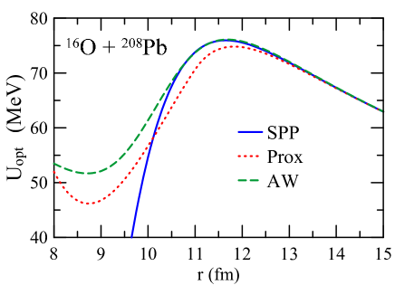
Figure 1: (Color online) Coulomb barriers for the bare potentials discussed in the text.

systen	parameter	AW	Prox	SP
	$V_{\rm\scriptscriptstyle B}$	21.1	20.0	20.8
8B+58Ni	$R_{\rm\scriptscriptstyle B}$	8.9	9.3	8.9
	$\hbar\omega$	4.6	4.0	4.1
	$V_{\rm\scriptscriptstyle B}$	20.6	19.3	21.2
4He+209Bi	$R_{\rm\scriptscriptstyle B}$	10.9	11.6	10.6
	$\hbar\omega$	5.3	4.7	5.6
	$V_{\rm\scriptscriptstyle B}$	21.6	20.6	20.9
6He+238U	$R_{\rm\scriptscriptstyle B}$	11.6	12.1	11.9
	$\hbar\omega$	4.5	3.8	4.0
	$V_{\rm\scriptscriptstyle B}$	30.4	29.0	29.8
6Li+209Bi	$R_{\rm\scriptscriptstyle B}$	11.1	11.6	11.3
	$\hbar\omega$	5.2	4.6	4.8
	$V_{\rm\scriptscriptstyle B}$	83.8	82.6	83.9
32S+100Mo	$R_{\rm\scriptscriptstyle B}$	10.8	10.9	10.7
	$\hbar\omega$	3.9	4.1	4.0
	$V_{\rm\scriptscriptstyle B}$	139.6	138.2	139.2
48Ca+154Sm	$R_{\rm\scriptscriptstyle B}$	12.0	12.1	12.0
	$\hbar\omega$	3.6	4.2	3.9

Table 1: Barrier parameters for different systems. $V_{\rm\scriptscriptstyle B}$ and $\hbar\omega$ are given in MeV and $R_{\rm\scriptscriptstyle B}$ is given in fm. We use boldface to indicate parameters which are very different for different potential models.

Clearly the Coulomb barriers generated by these potentials are quite different, especially in the inner region. They differ by their height and also by their widths. Thus, they are expected to lead to different tunneling probabilities at low energies. Similar differences can be found for other systems. To illustrate this point, Table 1 shows the barrier height ($V_{\rm\scriptscriptstyle B}$), radius ($R_{\rm\scriptscriptstyle B}$) and curvature ($\hbar\omega$) parameters for the systems: ⁸B+⁵⁸Ni, ⁴He+²⁰⁹Bi, ⁶He+²³⁸U, ⁶Li+²⁰⁹Bi, ³²S+¹⁰⁰Mo and ⁴⁸Ca+¹⁵⁴Sm. Clearly there are important differences in parameters associated with each of the bare potentials considered in our discussion.

In situations where two potentials produce very different barriers, one expects significant differences in the resulting fusion cross section. To check this point, we investigate the theoretical cross sections obtained with the above bare potentials for two systems: ⁶He + ²³⁸U and ⁴He + ²⁰⁹Bi. The barrier parameters associated with each of these potentials are considerably different, specially for the latter system.

The fusion cross section obtained by single-channel calculations (without channel-couplings) using the SP (solid lines), the AW (long-dashed lines) and the Proximity (short-dashed lines) potentials are shown in Fig. 2.

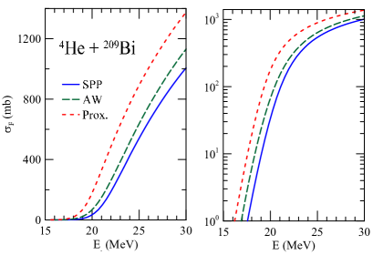
Figure 2: (Color online) Fusion cross sections for the ⁶He + ²³⁸U (top panels) and ⁴He + ²⁰⁹Bi (botom panels). The cross sections where obtained by single-channel calculations (no-couplings) using each of the bare potentials discussed in the text. To see clearly the behaviors above and below the barrier, the results are given in linear (left panels) and logarithmic (right panels) scales.

We notice clearly significant differences among the calculation with the three bare potentials. In particular the ⁴He case, the differences are indeed quite large. The fusion cross sections of the Borromean nucleus ⁶He calculated with the SP and the Proximity potential are close, but that obtained with the AW is much lower. Obviously in coupled channels analysis of fusion, the conclusions concerning the importance of the coupling is intimately related to the bare potential employed. Great care must be exercised in reaching these conclusions. What bare potentials one should use, will depend on a concomitant analysis of the cross section of other processes which are also sensitive to the barriers, such as breakup and elastic scattering.

A comparison with experimental fusion cross sections could indicate which bare potential gives more realistic results. However, comparing the above cross sections with data may be misleading, since these calculations do not incorporate coupled-channel effects, which are very important, specially for collision energies below the Coulomb barrier. Performing coupled channel calculations for the ⁶He projectile is too complicated as the continuum of the three-body system (${}^{4}{\rm He}+n+n$) is too hard to take into account. However, reliable coupled channel calculations for the ⁴He+²⁰⁹Bi system can easily be performed and the predictions of each bare potential can be compared with the experiment. We have performed coupled channel calculations including the couplings with all relevant channels, associated with the collective excited states of ²⁰⁹Bi. The results are shown in Fig. 3. The comparison indicates that the SP potential gives the best description of the data. The results of the Akÿuz-Winther potential are also quite satisfactory whereas those for the Proximity potential are much poorer.

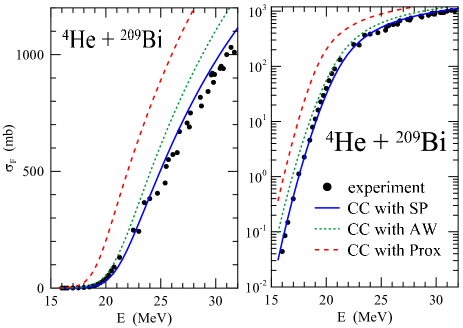
Figure 3: (Color online) Comparison of the experiment fusion cross section for the ⁴He + ²⁰⁹Bi system with theoretical cross sections obtained by coupled channel calculations using each of the bare potentials discussed in the text. As in the previous figures, the results are shown in linear (left panel) and logarithmic (right panel) scales.

To compare the above results with those involving other systems in an appropriate way, one should reduce the data, in order to eliminate the differences arising from size and charges of the collision partners. There are different proposals to reach this goal. A convenient one is to transform the cross sections into fusion functions, which depend on a dimensionless variable associated with the collision energy. One carries out the transformations Canto et al. (2009a, b):

$$E\,\rightarrow\,x=\frac{E-V_{\rm\scriptscriptstyle B}}{\hbar\omega}\ \ {\rm and}\ \ \sigma_{\rm\scriptscriptstyle F}\,\rightarrow\,F(x)=\frac{2E}{\hbar\omega\,R_{\rm\scriptscriptstyle B}^{2}}\times\sigma_{\rm\scriptscriptstyle F}.$$ (12)

If coupled channel effects can be neglected and Wong’s approximation Wong (1973) for the cross section holds, one obtains the Universal Fusion Function (UFF),

$$F_{0}(x)=\ln{\left[1+\exp{(2\pi x)}\right]}.$$ (13)

For light systems ($Z_{\rm\scriptscriptstyle P}Z_{\rm\scriptscriptstyle T}\ll 500$) Wong’s approximation is poor at sub-barrier energies. However, this approximation is much better above the barrier and the fusion functions are always close to the UFF in this energy region.

It is important to stress that the transformations of Eq. (12) depend on the barrier parameters of the bare potential. Usually, channel coupling effects have a major influence on the fusion cross section at sub-barrier energies. However, frequently, this influence is not so strong above the barrier. Thus, if the bare potential is correctly chosen, the experimental fusion function, obtained using the experimental cross section in Eq. (12), should be close to the UFF. That is,

$$\frac{2E}{\hbar\omega\,R_{\rm\scriptscriptstyle B}^{2}}\times\sigma_{\rm\scriptscriptstyle F}^{\rm\scriptscriptstyle exp}\simeq F_{0}(x).$$ (14)

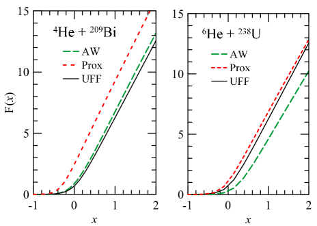
Figure 4: (Color online) Fusion functions for the AW and the Proximity potentials, obtained through single-channel calculations, as explained in the text.

We use a similar procedure to compare the cross sections of Fig. 2 in terms of fusion functions. We consider the same systems and use the barrier parameters of the SP potential to carry out the reduction. The fusion functions associated with theoretical cross sections obtained by single channel calculations with the AW and Proximity potentials are shown in Fig. 4. We leave out the fusion function associated with the SP potential itself, because it is almost indistinguishable from the UFF. This is because Wong’s approximation is very accurate in the above-barrier region shown in detail in the figure. If the AW and the Proximity potentials were equivalent to the SP one, their fusion functions would also be very close to the UFF. We see clearly the sensitivity of $F(x)$ to the bare potential employed. In the ⁴He case, the calculation of $F(x)$ with the AW bare potential is close to the UFF, while $F(x)$ calculated with the Proximity bare potential it is quite different from UFF. The situation is inverted in the ⁶He fusion case. Here the AW bare potential gives a $F(x)$ much lower than the UFF, while the Proximity potential is practically identical with the UFF. This finding only strengthens our argument that there is great sensitivity of near-barrier fusion to the bare potential. A bad choice of the bare potential may lead to wrong conclusions about the behavior of $\sigma_{\rm\scriptscriptstyle F}$.

What causes the differences among the bare potentials used in this paper? We believe the major difference resides in the fact that the SP potential, which is the double folding interaction with realistic densities, is more faithful in catching the essentials of the nucleus-nucleus interaction. In fact, it is based on experimentally determined densities and there are no approximations involved, in contrast to the AW potential, which uses an analytical form of these densities, and employs further approximations to allow an analytical evaluation of the double folding integral. The Proximity potential, being constructed for epidermic systems, with diffuseness much smaller than the radius of a given nucleus, is reasonable for the heavy targets considered, but fails for the light projectile. The systems studied in the previous figures have very unusual densities. On the one hand, ⁴He is a very compact nucleus whereas the density of ⁶He is influenced by the two neutron halo. To illustrate this point, we compare the experimental densities of ⁶He Vries et al. (1987), used in the SP potential, with a gaussian density that does not include the contribution of the halo. This schematic density is given by a gaussian normalised by the condition $A=6$ and with r.m.s. radius corresponding to that of ⁴He scaled by the factor $(6/4)^{1/3}$, as in Ref. Cardenas et al. (2003). The two densities are compared in Fig. 5 (a). They are indeed very different. The fusion cross sections obtained with the SP potential using these densities are exhibited in Fig. 5 (b). As expected, the cross sections are considerably different. This clearly shows the importance of using realistic densities in the calculation of the bare potential.

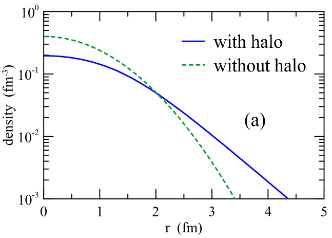
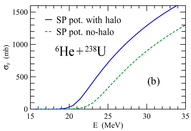
Figure 5: (Color online) panel (a): Densities of ⁶He taking into account the two-neutron halo structure (solid line), and treating it as a tightly bound nucleus. For details, see the text; panel (b): Fusion cross sections for the ⁶He+²³⁸U system obtained from single-channel calculations with the SP potential, using the two densities of the previous figure.

IV Extracting barrier parameters from above-barrier data

Attempts have been made to infer the parameters of the bare potential using fusion cross section measurements at above-barrier energies (see, e.g. Ref.  Kolata et al. (1998)). If one uses the classical approximation for the transmission factor,

$$T_{l}(E) = 1,\qquad{\rm for}\ E>V_{\rm\scriptscriptstyle B}(l)$$ (15)

$$= 0,\qquad{\rm for}\ E\leq V_{\rm\scriptscriptstyle B}(l),$$ (16)

where $V_{\rm\scriptscriptstyle B}(l)$ stands for the height of the barrier of the effective potential at the angular momentum $l$, the partial-wave series can easily be evaluated. One then gets the fusion cross section,

$$\sigma_{\rm\scriptscriptstyle F}=\pi\,R_{\rm\scriptscriptstyle B}^{2}\ \left[1-\frac{V_{\rm\scriptscriptstyle B}}{E}\right],$$ (17)

with $V_{\rm\scriptscriptstyle B}\equiv V_{\rm\scriptscriptstyle B}(l=0)$. Thus, plotting $\sigma_{\rm\scriptscriptstyle F}$ vs. $1/E$, the barrier height and radius can be immediately obtained from the interceptions of the straight line with the two axis. It intercepts the $1/E$ axis at $1/V_{\rm\scriptscriptstyle B}$ and the $\sigma_{\rm\scriptscriptstyle F}$ axis at $\pi R_{\rm\scriptscriptstyle B}^{2}$.

Before further discussions of this procedure, one has to decide how much above the barrier one should take the data. Above some critical energy, the highest angular momenta should be excluded from the partial-wave summation. This is because at these angular momenta the effective optical potential,

$$V_{l}(r)=V_{\rm\scriptscriptstyle N}(r)+V_{\rm\scriptscriptstyle C}(r)+\frac{\hbar^{2}}{2\mu\,r^{2}}\,l(l+1),$$ (18)

with $V_{\rm\scriptscriptstyle N}(r)$ and $V_{\rm\scriptscriptstyle C}(r)$ standing respectively for the bare nuclear potential and the Coulomb interaction, does not have a pocket. Thus the projectile cannot be captured and fusion does not take place. The fusion cross section is then in another energy regime, where it does not have a linear dependence on $1/E$. On the other hand, at energies just above the barrier, the classical approximation for the transmission factor is inaccurate. To choose the energy region where the cross section has the desired linear behavior, one should compare the cross section of Eq. (17) with its quantum mechanical counterpart. In order to get a system independent answer, we make this comparison using reduced cross sections. That is, we compare the UFF with its high energy limit, where tunnelling effects can be neglected. It can be easily checked that at high enough energies ($x\gg 1$) Eq. (13) can be approximated by its limit,

$$F_{0}(x\rightarrow\infty)\rightarrow F_{0}^{\rm cl}(x)=2\pi\,x.$$ (19)

Figure 6: (Color online) The Universal Fusion Fusion (solid line) and its high energy limit (dashed line).

In Fig. (6) we compare the exact form of the UFF with its asymptotic limit. The comparison indicates that the asymptotic expression can be safely used for $x>0.5$. That is, for energies $\hbar\omega/2$ above the barrier. Since $\hbar\omega\sim 4$ MeV, one should take data starting at about 2 MeV above the barrier.

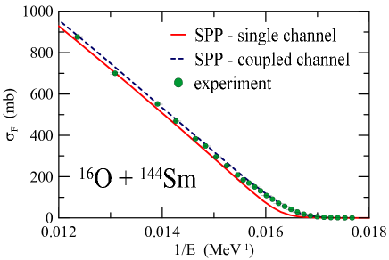
Figure 7: (Color online) Fusion cross sections for the ¹⁶O+¹⁴⁴Sm system plotted against $1/E$. The solid line corresponds to a single-channel calculation with the SP potential whereas the dashed line are results of a coupled channel calculation using the same bare potential. The experimental data of Leigh et al. Leigh et al. (1995) are also shown.

	parab. fit	single-channel	CC	data
$V_{\rm\scriptscriptstyle B}$ (MeV)	61.4	61.2	60.6	60.8
$R_{\rm\scriptscriptstyle B}$ (fm)	10.9	10.6	10.6	10.6

Table 2: Barrier parameters for the ¹⁶O+¹⁴⁴Sm system. $V_{\rm\scriptscriptstyle B}$ is given in MeV and $R_{\rm\scriptscriptstyle B}$ is given in fm.

The difficulty with this procedure is that the experimental cross section is usually influenced by channel coupling effects. Although these effects are much more important below the Coulomb barrier, they may affect the cross section at above-barrier energy. In this case, the parameter extracted from the cross section would be associated with some sort of effective barrier without any practical utility. Thus, the influence of channel couplings above the barrier should be checked.

As a first step, we consider the trivial case of the ¹⁶O+¹⁴⁴Sm system, where these effects are known to be very weak. In Fig. 7 we compare the experimental fusion cross section of Leigh et al. Leigh et al. (1995) with results of the single-channel (solid line) and coupled channel (dashed line) calculations. In both cases, we used the SP as the bare potential. As expected, the single-channel cross section is close to the coupled channel one and to the data. Fitting straight lines to the linear region of the cross section, we extracted the height and the radius of the barrier, for the two calculations and for the data. The results are shown in table 2, together with correct values of the barrier parameters. The latter was obtained fitting a parabola to the barrier of the total optical potential (sum of the bare nuclear potential with the Coulomb interaction). The radii obtained from the $1/E$ dependence of the two calculations and the data are quite close to the correct radius of the barrier. The three are identical and they differ from the exact value by 0.3 fm. The barrier heights, however, are not so close. The height extracted from the data is 0.6 MeV below the correct height. We should keep in mind that the purpose of this procedure is to extract the parameters of the bare potential from the linear fit of the data and even in this extreme case of weak coupling the barrier height differs from the correct value by 0.6 MeV. This example does not encourage the use of the method in situations where the couplings are not so weak.

Now we study another example, where coupling effects are known to influence the cross section above the barrier. We consider collisions of the halo-nucleus ⁶He with a ²⁰⁹Bi target. In Fig. 8 we show the data of Kolata et al. Kolata et al. (1998) plotted against $1/E$, and the corresponding linear fit. From this fit we have obtained the radius and the height of the barrier. The results are shown in table 3, in comparison with the barrier parameters associated with the three potentials of section II. In each case, the parameters were obtained fitting a parabola to the barrier of the total optical potential.

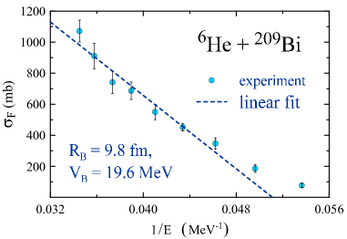
Figure 8: (Color online) Experimental fusion cross section for the ⁶He + ²⁰⁹Bi system Kolata et al. (1998), plotted against $1/E$. The dashed line corresponds to a linear fit, to the expression of Eq. (17). The barrier height and radius obtained are indicated within the figure.

	AW	Prox	SP	experiment
$V_{\rm\scriptscriptstyle B}$ (MeV)	20.0	19.0	20.9	19.6
$R_{\rm\scriptscriptstyle B}$ (fm)	11.3	11.8	11.9	9.8

Table 3: Barrier parameters extracted from above-barrier data of the ⁶He + ²⁰⁹Bi system, in comparison with the corresponding values for the three bare potentials discussed in the text.

The discrepancy between the barrier height extracted from the data and that for the SP potential is not larger than the discrepancies among the predictions of the three bare potentials. However, $1/E$ fit leads to a very wrong barrier radius. Independently of the option for the bare potential, the radius taken from the above-barrier data is $\sim 2$ fm too small. This deviation arises from the strong suppression of the fusion cross section above the barrier, arising from breakup couplings Canto et al. (2009a, b).

V Conclusions

In this paper we report on a detailed study of the bare optical potentials frequently employed in the analysis of near-barrier heavy-ion fusion reactions.

We have found that these potentials give rise to different fusion barriers. They consequently lead to different conclusions about the effect of the channel couplings when coupled channels calculation of the fusion cross section is perforrmed. We have further found that folding potentials based on realistic densities tend to be more reliable.

We have further shown that the extraction of $R_{\rm\scriptscriptstyle B}$, $V_{\rm\scriptscriptstyle B}$ from $1/E$ plots may be accurate within $\sim 0.5$ fm and $\sim 0.5$ MeV when channel coupling effects above the barrier are very small. However, if coupled channels affect the fusion cross section above the barrier, this method may lead to meaningless barrier parameters.

Acknowledgements

The authors would like to thank the financial support from CNPq, CAPES, FAPERJ, FAPESP and the PRONEX.

References

- Canto et al. (2006) L. F. Canto, , P. R. S. Gomes, R. Donangelo, and M. S. Hussein, Phys. Rep. 424, 1 (2006).
- Hagino et al. (2000) K. Hagino, A. Vitturi, C. H. Dasso, and S. M. Lenzi, Phys. Rev. C 61, 037602 (2000).
- Diaz-Torres and Thompson (2002) A. Diaz-Torres and I. J. Thompson, Phys. Rev. C 65, 024606 (2002).
- Diaz-Torres et al. (2003) A. Diaz-Torres, I. J. Thompson, and C. Beck, Phys. Rev. C 68, 044607 (2003).
- Kuo and Brown (1966) T. T. S. Kuo and G. E. Brown, Nucl. Phys. 85, 40 (1966).
- Bertsch et al. (1977) G. F. Bertsch, J. Borysowicz, H. McManus, and W. G. Love, Nucl. Phys. A284, 399 (1977).
- Chamon et al. (1997) L. C. Chamon, D. Pereira, M. S. Hussein, M. A. C. Ribeiro, and D. Galetti, Phys. Rev. Lett. 79, 5218 (1997).
- Chamon et al. (2002) L. Chamon, B. Carlson, L. Gasques, D. Pereira, C. D. Conti, M. Alvarez, M. Hussein, M. C. Ribeiro, E. R. Jr., and C. Silva, Phys. Rev. C 66, 014610 (2002).
- Perey and Buck (1962) F. Perey and B. Buck, Nucl. Phys. 32, 353 (1962).
- Blocki et al. (1977) J. Blocki, J. Randrup, W. J. Swiatecki, and C. F. Tsang, Ann. Phys. (NY) 105, 427 (1977).
- Canto et al. (2009a) L. F. Canto, P. Gomes, J. Lubian, L. Chamon, and E. Crema, J. Phys. G: Nucl. Part. Phys. 36, 015109 (2009a).
- Canto et al. (2009b) L. F. Canto, P. Gomes, J. Lubian, L. Chamon, and E. Crema, Nucl. Phys. A 821, 51 (2009b).
- Wong (1973) C. Y. Wong, Phys. Rev. Lett. 31, 766 (1973).
- Vries et al. (1987) H. D. Vries, C. D. Jager, and C. D. Vries, At. Data Nucl. Data Tables 36, 495 (1987).
- Cardenas et al. (2003) W. H. Z. Cardenas, L. F. Canto, N. Carlin, R. Donangelo, and M. S. Hussein, Phys. Rev. C68, 054614 (2003).
- Kolata et al. (1998) J. J. Kolata, V. Guimarães, D. Peterson, P. Santi, R. White-Stevens, P. A. De Young, G. F. Peaslee, B. Hughey, B. Atalla, M. Kern, et al., Phys. Rev. Lett. 81, 4580 (1998).
- Leigh et al. (1995) J. R. Leigh, M. Dasgupta, D. J. Hinde, J. C. Mein, C. R. Morton, R. C. Lemmon, J. P. Lestone, J. O. Newton, H. Timmer, J. X. Wei, et al., Phys. Rev. C52, 3151 (1995).