Data Mining using Unguided Symbolic Regression on a Blast Furnace Dataset

Abstract

In this paper a data mining approach for variable selection and knowledge extraction from datasets is presented. The approach is based on unguided symbolic regression (every variable present in the dataset is treated as the target variable in multiple regression runs) and a novel variable relevance metric for genetic programming. The relevance of each input variable is calculated and a model approximating the target variable is created. The genetic programming configurations with different target variables are executed multiple times to reduce stochastic effects and the aggregated results are displayed as a variable interaction network. This interaction network highlights important system components and implicit relations between the variables. The whole approach is tested on a blast furnace dataset, because of the complexity of the blast furnace and the many interrelations between the variables. Finally the achieved results are discussed with respect to existing knowledge about the blast furnace process.

1 Introduction

Data mining is the process of finding interesting patterns in large datasets to gain knowledge about the data and the process it originates from. This work concentrates on the identification of relevant variables which is mainly referred to as variable or feature selection ([1] provides a good overview about the field). Usually a large set of variables is available in datasets to model a given fact and it can be assumed that only a specific subset of these variables is actually relevant. Although there are often no details given on how variables are related, an identified set of relevant variables is easy to understand and can already increase the knowledge about the dataset considerably. However, determining the subset of relevant variables is non-trivial especially if there are non-linear or conditional relations. Implicit dependencies between variables further hamper the identification of relevant variables as this ultimately leads to multiple sets of different variables that are equally possible.

In this paper genetic programming (GP) [4], a general problem solving meta-heuristic, is used for data mining. GP is well suited for data mining because it produces interpretable white box models and automatically evolves the structure and parameters of the model [4]. In GP feature selection is implicit because fitness-based selection makes models containing relevant variables more likely to be included in the next generation. As a consequence, references to relevant variables are more likely than references to irrelevant ones. This implicit feature selection also removes variables which are pairwise highly correlated but irrelevant to describe a given relation. However, if pairwise correlated and relevant variables exists in the dataset, GP does not recognize that one of the variables can be removed and keeps both.

In this work symbolic regression analysis is executed multiple times to reveal sets of relevant variables and to reduce stochastic events. Additionally aggregated characteristics about the whole algorithm run are used to extract information about the dataset, instead of solely using the identified model. In section 2 a overview of metrics used to calculate the variable relevance is given and a new frequency-based variable relevance metric is proposed. Section 3 outlines the experimental setup, the blast furnace dataset and the parameters for the GP runs. Section 4 presents and discusses the achieved results and section 5 concludes the paper.

2 Variable Relevance Metrics for GP

Knowledge about the minimal set of input variables necessary to describe a given dependent variable is often very valuable for domain experts and can improve the understanding of the examined system. In the case of linear models the relevance of variables can be detected by shrinkage methods [2]. If genetic programming is used for the analysis of relevant variables not only linear relations but, based on the set of allowed symbols, also non-linear or conditional impact factors can be detected. The extraction of the variable relevance from GP runs is not straightforward and highly depends on the metrics used to measure the variable importance.

Two variants to approximate the relevance of variables for genetic programming have been described in [12]. Although both metrics have been designed to measure population diversity they can be used to estimate the variable relevance. The frequency-based approach either uses the sum of variable references in all models or the number of models referencing a variable. The second, impact-based metric uses the information present in the variable to estimates its relevance. The idea is to manipulate the dataset to remove the variable for which the impact should be calculated (e.g., by replacing all occurrences with the mean of the variable) and to measure the response differences between the original model and the manipulated one.

In [10] two different definitions of variable relevance are proposed. The presence weighted variable importance calculates the relative number of models, identified and manually selected by one or multiple ParetoGP [8] runs, which reference this variable. The fitness-weighted variable importance metric also uses the presence of variables in identified models, but additionally takes the fitness of the identified models into account [7]. As the authors state this eliminates the need of manually selecting models because the aggregated and weighted score of irrelevant variables should be much smaller than the overall score of relevant variables.

2.1 Extension of Frequency-based Variable Relevance for GP

The frequency-based variable relevance $\text{rel}_{\text{freq}}$ is also based on the variable occurrence over multiple models but in contrast to the other metrics the whole algorithm run is used to calculate the variable relevance. The frequency of a variable $x_{i}$ in a population of models is calculated by counting the references to this variable over all models $m$ (Equation 1,2). The frequency is afterwards normalized by the total number of variable references in the population (Equation 3) and the resulting frequencies are averaged over all generations (Equation 4).

$$\text{CountRef}(x_{i},m)=\begin{cases}1+\sum_{b\in\text{Subtrees}(m)}\text{CountRef}(x_{i},b)\text{ , }if\text{ Symbol}(m)=x_{i}\\ 0+\sum_{b\in\text{Subtrees}(m)}\text{CountRef}(x_{i},b)\text{ , }if\text{ Symbol}(m)\neq x_{i}\\ \end{cases}$$ (1)

$$\text{frequ}(x_{i},\text{Pop})=\sum_{m\in\text{Pop}}\text{CountRef}(x_{i},m)$$ (2)

$$\text{rel}_{\text{frequ}}(x_{i},\text{Pop})=\frac{\text{freq}(x_{i},\text{Pop)}}{\sum_{k=1}^{n}\text{freq}(x_{k},\text{Pop})}$$ (3)

$$\text{relevance}(x_{i})=\frac{1}{G}\sum_{g=1}^{G}\text{rel}_{\text{freq}}(x_{i},\text{Pop}_{g})$$ (4)

Tracing the relative variable frequencies over the whole GP run and visualizing the results is aimed to lead to insights into the dynamics of the GP run itself. Figure 1 shows the trajectories of relative variable frequency for the blast furnace dataset described in section 3.1. It can be already seen that the relevance of variables varies during the GP run. In the beginning two variables (the hot blast amount and the hot blast $O_{2}$ proportion) are used in most models, but after 100 generations the total humidity overtops these two. The advantage of calculating the variable relevance over the whole run instead of using only the last generation is that the dynamic behavior of GP is taken into account.

Because of the non-deterministic nature of the GP process the relevance of variables typically differs over multiple independent GP runs. Implicit linear or non-linear dependencies between input variables are another possible reason for these differences. Therefore, the variable relevances of one single GP run are not representative. It is desirable to analyze variable relevance results over multiple GP runs in order to know which variables are most likely necessary to explain the target variable and which variables have a high relevance in single runs only by chance. Therefore, all GP runs are executed multiple times and the results are aggregate to minimize stochastic effects.

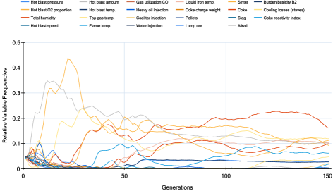
Figure 1: Relative Variable Frequencies of one single GP run for the blast furnace dataset.

3 Experiments

The frequency-based variable relevance metric and data mining approach is tested on a complex industrial system. The general blast furnace and the physical and chemical reactions occurring in the blast furnace are quite well known. However, on a detailed level many of the inter-relationships of different parameters and the occurrence of fluctuations and unsteady behavior in the blast furnace are not totally understood. Therefore, the knowledge about relevant variables and accurate approximations of process variables are of special importance and were calculated using repeated GP runs on the blast furnace dataset.

3.1 Blast Furnace Dataset

The blast furnace is the most common process to produce hot metal globally. More than 60% of the iron used for steel production is produced in the blast furnace process [6]. The raw materials for the production of hot metal enter the blast furnace via two paths. At the top of the blast furnace ferrous oxides and coke are charged in alternating layers. The ferrous oxides include sinter, pellets and lump ore. Additionally feedstock to adjust the basicity is also charged at the top of the blast furnace. In the lower area of the blast furnace the hot blast (air, $1200\,^{\circ}\mathrm{C}$) and reducing agents are injected through tuyeres. These reducing agents include heavy oil, pulverized coal, coke oven or natural gas, coke tar and waste plastic and are added to substitute coke. The products of the blast furnace are liquid iron (hot metal) and the liquid byproduct slag tapped at the bottom and blast furnace gas which is collected at the top. For a more detailed description of the blast furnace process see [9].

The basis of our analysis is a dataset containing hourly measurements of a set of variables of the blast furnace listed in Table 1. The dataset contains almost 5500 rows; rows 100–3800 are used for training and rows 3800–5400 for testing. Only the first half of the training set (rows 100–1949) is used to determine the accuracy of a model. The other half of the training set (rows 1950–3800) is used for validation and selection of the final model. The dataset cannot be shuffled because the observations are measured over time and the nature of the process is implicitly dynamic.

Group	Variables
Hot blast	pressure	amount
	$O_{2}$ proportion	speed
	temperature	total humidity
Tuyere Injection	amount of heavy oil	amount of water
	amount of coal tar
Charging	coke charge weight	amount of sinter
	amount of pellets	amount of coke
	amount of lump ore	burden basicity B2
	coke reactivity index
Tapping	hot metal temperature	amount of slag
	amount of alkali
Blast furnace top gas	temperature	gas utilization CO
Process parameters	melting rate	cooling losses (staves)

Table 1: Variables included in the blast furnace dataset.

3.2 Algorithmic Settings

Unguided symbolic regression treats each of the variables listed in Table 1 as the target variable in one GP configuration and all remaining variables are allowed as input variables. This leads to 23 different configurations, one for each target variable. For each configuration 30 independent runs have been executed on a multi processor blade system to reduce stochastic effects. Table 2 lists the algorithm parameters for the different GP configurations. The resulting model of the GP run is that one with the largest $R^{2}$ on the validation set and gets linearly scaled [3] to fit the location and scale of the target variables. The approach described in this contribution was implemented and tested in the open source framework HeuristicLab [11].

Parameter	Value
Population size	1000
Max. generations	150
Parent selection	Tournament (group size =7)
Replacement	1-Elitism
Initialization	PTC2 [5]
Crossover	Sub-tree-swapping
Mutation rate	15%
Mutation operators	One-point and Sub-tree replacement
Tree constraints	Max. expression size = 100
	Max. expression depth = 10
Model selection	Best on validation
Stopping criterion	Max. generations reached
Fitness function	$R^{2}$ (maximization)
Function set	+,-,*,/,avg,log,exp
Terminal set	constants, variable

Table 2: Genetic programming parameters for the blast furnace dataset.

4 Results

A box plot of the model accuracies ($R^{2}$) over 30 independent runs for each target variable of the blast furnace dataset is shown in Figure 2. The $R^{2}$ values are calculated from the predictions of the best model (selected on the validation set) on the test set for each run. Whiskers indicate four times the interquartile range, values outside of that range are indicated by small circles in the box-plot. Almost all models for the hot blast pressure result in a perfect approximation ($R^{2}\approx 1.0$). Very good approximations are also possible for the $O_{2}$ proportion of the hot blast and for the flame temperature. On the other hand the hot blast temperature, the coke reactivity index and the amount of water injected through tuyeres cannot be modeled accurately using symbolic regression.

Figure 2: Box-plot of $R^{2}$ value on the test set of models for the blast furnace dataset.

4.1 Variable Interaction Network

The variable interaction network obtained from the GP runs is shown in Figure 3. For each target variable the three most relevant input variables are indicated by an arrow pointing to the target variable. Arrows in both directions are an indication that the pair of variables is strongly related; the value of the first variable is needed to approximate the value of the second variable and vice versa. Variables that have many outgoing arrows play a central role in the process and can be used to approximate many other variables. In the blast furnace network central variables are the melting rate, the amount of slag, the amount of injected heavy oil, the amount of pellets, and the hot blast speed and its $O_{2}$ proportion. The unfiltered variable interaction network must be interpreted in combination with the box plot in Figure 2 because the significance (not in the statistical sense) of arrows pointing to variables which cannot be approximated accurately is rather low (e.g., the connection between the coke reactivity index and the burden basicity B2).

Figure 3: Relationships of blast furnace variables identified with unguided symbolic regression.

4.2 Detailed Results

The variable interaction network for the blast furnace process provides a good overview of the blast furnace process. Exemplary the influence factors obtained by unguided symbolic regression on the melting rate are analyzed and compared to the influences known by domain experts.

The melting rate is primarily a result of the absolute amount of $O_{2}$ injected into the furnace and is also related to the efficiency of the furnace. A crude approximation for the melting rate is

$$\frac{\text{Total amount of }O_{2}}{[220\ldots 245]}$$ (5)

When the furnace is working properly the melting rate is higher ($O_{2}/220$), when the furnace is working inefficiently the melting rate decreases ($O_{2}/245$) and high cooling losses can be observed. Additional factors that are known to affect the melting rate are the burden composition and the amount of slag. The identified models show a strong relation of the melting rate with the hot blast parameters (data not shown). The melting rate is used in models for the hot blast parameters: pressure, $O_{2}$-proportion, amount, and the total humidity which is largely determined by the hot blast. In return the hot blast parameters play an important role in the model for the melting rate.

Equation 6 shows a model for the melting rate with a rather high squared correlation coefficient of 0.89 that has been further simplified by omitting uninfluential terms and manual pruning. The generated model 6 (constants $c_{i},i=1..8$ are omitted for better readability) also indicates the known relation of the melting rate and the amount of $O_{2}$. Additionally the cooling losses, the amount of lump ore and the gas utilization of CO have been identified as factors connected to the melting rate.

$$\begin{split}\text{Melting rate}=&{}\log(c_{0}\times\text{Temp}_{\text{HB}}\times O_{2}\text{-prop}_{\text{HB}}\times\\ &(c_{1}\text{Cool. loss}+c_{2}\text{Amount}_{\text{HB}}+c_{3})+c_{4}\times\text{Gas util}_{CO}\\ &\times(c_{5}\text{Lump ore}+c_{6})\times(c_{7}\text{Amount}_{\text{HB}}+c_{8}))\end{split}$$ (6)

5 Conclusion

Many variables in the blast furnace process are implicitly related, either because of underlying physical relations or because of the external control of blast furnace parameters. Examples for variables with implicit relations to other variables are the flame temperature or the hot blast parameters. Usually such implicit relations are not known a-priori in data-based modeling scenarios but could be extracted from the variable relevance information collected from multiple GP runs.

Using an unguided symbolic regression data mining approach several models have been identified that approximate the observed values in the blast furnace process rather accurately. In some cases the data-based models approximate known underlying physical relations, but in general the statistical models produced by the data mining approach do not match the physical models perfectly. A possible enhancement could be the usage of physical units in the GP process to evolve physically correct models.

Currently the variable relevance information is used to determine the necessary variable set to model the target variable. The experiments also lead to a number of models describing several components of the blast furnace. The generated models can be used to extract information about implicit relations in the dataset to further reduce and disambiguate the set of relevant input variables. Additionally the information about relations between input variables can be used to manually transform symbolic regression models to lower the number of alternative representation of the same causal relationship. However, the implementation of software that uses such models of implicit relations or manually declared a-priori knowledge intelligently, to simplify symbolic regression models, or to provide alternative semantically equivalent representations of symbolic regression models, is left for future work.

Acknowledgments

This research work was done within the Josef Ressel-center for heuristic optimization “Heureka!” at the Upper Austria University of Applied Sciences, Campus Hagenberg and is supported by the Austrian Research Promotion Agency (FFG).

References

- [1] Guyon, I., Elisseeff, A.: An introduction to variable and feature selection. Journal of Machine Learning Research 3, 1157–1182 (March 2003)
- [2] Hastie, T., Tibshirani, R., Friedman, J.: The Elements of Statistical Learning - Data Mining, Inference, and Prediction. Springer (2009), second Edition
- [3] Keijzer, M.: Scaled symbolic regression. Genetic Programming and Evolvable Machines 5(3), 259–269 (Sep 2004)
- [4] Koza, J.R.: Genetic Programming: On the Programming of Computers by Means of Natural Selection. MIT Press, Cambridge, MA, USA (1992)
- [5] Luke, S.: Two fast tree-creation algorithms for genetic programming. IEEE Transactions on Evolutionary Computation 4(3), 274–283 (Sep 2000)
- [6] Schmöle, P., Lüngen, H.B.: Einsatz von vorreduzierten Stoffen im Hochofen: metallurgische, ökologische und wirtschaftliche Aspekte. Stahl und Eisen 4(127), 47–56 (2007)
- [7] Smits, G., Kordon, A., Vladislavleva, K., Jordaan, E., Kotanchek, M.: Variable Selection in Industrial Datasets Using Pareto Genetic Programming, Genetic Programming, vol. 9, pp. 79–92. Springer US (2006)
- [8] Smits, G.F., Kotanchek, M.: Pareto-front exploitation in symbolic regression. In: O’Reilly, U.M., Yu, T., Riolo, R., Worzel, B. (eds.) Genetic Programming in Theory and Practice II, pp. 283–299. Springer (2005)
- [9] Strassburger, J.H., Brown, D.C., Dancy, T.E., Stephenson, R.L. (eds.): Blast furnace - theory and practice. Gordon and Breach Science Publishers, New York (1969), second Printing August 1984
- [10] Vladislavleva, K., Veeramachaneni, K., Burland, M., Parcon, J., O’Reilly, U.M.: Knowledge mining with genetic programming methods for variable selection in flavor design. In: Proceedings of the Genetic and Evolutionary Computation Conference (GECCO 2010). pp. 941–948 (2010)
- [11] Wagner, S.: Heuristic Optimization Software Systems - Modeling of Heuristic Optimization Algorithms in the HeuristicLab Software Environment. Ph.D. thesis, Institute for Formal Models and Verification, Johannes Kepler University, Linz, Austria (2009)
- [12] Winkler, S.M.: Evolutionary System Identification - Modern Concepts and Practical Applications. No. 59 in Reihe C - Technik und Naturwissenschaften, Trauner Verlag, Linz (2008)