Polar plumes’ orientation and the Sun’s global magnetic field

Abstract

Aims. We characterize the orientation of polar plumes as a tracer of the large-scale coronal magnetic field configuration. We monitor in particular the north and south magnetic pole locations and the magnetic opening during 2007–2008 and provide some understanding of the variations in these quantities.

Methods. The polar plume orientation is determined by applying the Hough-wavelet transform to a series of EUV images and extracting the key Hough space parameters of the resulting maps. The same procedure is applied to the polar cap field inclination derived from extrapolating magnetograms generated by a surface flux transport model.

Results. We observe that the position where the magnetic field is radial (the Sun’s magnetic poles) reflects the global organization of magnetic field on the solar surface, and we suggest that this opens the possibility of both detecting flux emergence anywhere on the solar surface (including the far side) and better constraining the reorganization of the corona after flux emergence.

Conclusions.

1 Introduction

The plasma $\beta$ in the corona is low enough that, on time scales much greater than the wave-crossing times and on spatial scales much greater than the small-scale turbulence driven by photospheric braiding of the field lines, it is almost force free. The large-scale, slowly-evolving coronal magnetic field is then predominantly determined by the distribution of the magnetic field in the photosphere below and by the way it connects to the solar wind and parker spiral above. This is the basis for attempts to reconstruct the coronal magnetic field using photospheric vector magnetograms (for a review see Wiegelmann & Sakurai, 2012). Additional information on the spatial structure of the coronal magnetic field is contained in EUV and X-ray images of the solar corona (see Aschwanden et al., 2008), which can be used to test field extrapolations (see De Rosa et al., 2009).

For global extrapolations of the Sun’s magnetic field (for a recent review see Mackay & Yeates, 2012), the total amount of open flux Lockwood et al. (2004), the location of the heliospheric current sheet (e.g., Virtanen & Mursula, 2010; Erdős & Balogh, 2010), and the location of coronal holes (e.g., Levine, 1982) are additional constraints. For example, Wang et al. (1997) studied the evolution of the coronal streamer belt during the 1996 activity minimum and compared the results to extrapolations, including those based on the evolution of the photospheric magnetic field from a flux transport simulation (see, e.g., Mackay & Yeates, 2012). They found that changes in the structure of the streamers correspond to flux emergence, in such a way that both the longitude of emergence and the orientation of the newly emerged bipole to the pre-existing coronal fields affect the streamer’s structure.

In this paper we discuss a further constraint for models of the coronal magnetic field, which is induced by the orientation of polar plumes, predominantly elongated striations seen in coronagraphs mostly above the polar caps. The orientation of these plumes is aligned with the magnetic field and can be directly compared with the orientation of field lines from extrapolations of the coronal magnetic field. We perform an analysis related to the work of Wang et al. (1997) using EUV images from SOHO and concentrating on polar plumes. This restricts our study to times of solar activity minimum, because these are the times when the plumes are readily visible. Here, we use five parameters to characterize the orientation of all plumes visible in one hemisphere at any given time. The first two parameters are the longitude and latitude at which the inclination of the plumes is exactly radial: on the assumption that the plumes are field-aligned this corresponds to the magnetic north (or south) pole. The three other parameters characterize how rapidly the plumes tilt away from radial with increasing distance from the pole as a function of longitude. These parameters measure the magnetic opening factor of the polar cap field. To lowest order, we can determine two such opening factors in mutually orthogonal magnetic meridional planes and the longitudinal orientation of these planes. Specific details, including how these parameters were measured, are given in Section 2.

In Section 3 we give the time history of the evolution of the location of the magnetic north and south poles, as well as the opening factors. This evolution is compared with current sheet source surface extrapolations (Zhao & Hoeksema, 1995) based on surface flux transport simulations(Jiang et al., 2010). We find reasonable qualitative agreement, with the differences suggesting ways the surface flux transport model can be refined. In Section 4 we note that the orientation of the coronal plumes is thus sensitive to flux emergence anywhere on the Sun (as Wang et al., 1997, found for streamers). As with the streamers, the temporal variation of the plume orientation is sensitive to flux emergence anywhere on the disk. The changes depend on where the flux emerges, how it is oriented in relation to the pre-existing field, and how the field of the bipole and the pre-existing field interact. Although not pursued in this paper, this suggests that “far-side imaging” of flux emergence and studies of the interaction between the emerging flux and pre-existing field using coronal images is a possibility. Section 5 briefly presents our conclusions.

2 Methods

2.1 Determination of the polar coronal field inclination

The raw data for this study are sequences of EUVI and EIT images at 171 Å taken from April 3 2007 to May 8, 2008, i.e., during the minimum between cycles 23 and 24. Our aim is to use the orientation of the polar plumes as a diagnostic of the Sun’s large-scale magnetic field. The procedure is to first analyze individual images. For the STEREO/EUVI and SOHO/EIT 171Å images, we have calculate the Hough-wavelet transform as described in de Patoul et al. (2013) to measure the inclination of the plumes.

Briefly, the images have been preprocessed by suitable background subtraction and mapped into cylindrical coordinates $(r,\phi)$ with respect to the solar disk center. The images have then been transformed using a Hough-wavelet transform to a translational distance ($\rho$) and an inclination ($\theta$).

As is shown in de Patoul et al. (2013), power maxima in the transformed map are generated at singular positions ($\rho,\theta$) when the projected plume structure is inclined by angle $\theta$ with respect to the radial, and its foot point is projected to colatitude $\vartheta_{c}=\rho/\cos\theta-\Delta\tan\theta$. Here, $\Delta$ is the distance of a virtual Hough center above the solar surface in units of solar radii. Since the inclination angle $\theta$ of the plumes varies smoothly with colatitude $\vartheta_{c}$, or likewise with $\rho$, the power maxima lie in Hough space almost along a straight line $\theta=u\rho+v$. The $\rho$-value where this line crosses $\theta=0$ (intercept $-v/u$) gives the special colatitude $\tilde{\vartheta}_{c}$ of the foot-point from which a plume is projected perpendicular to the limb. The slope $u$ of this line corresponds to the change in the plume’s inclination $\iota$ with foot-point colatitude $\vartheta_{c}$. Introducing the co-inclination angle $\iota_{c}=\pi/2-\iota$ which vanishes at the pole, the parameter $u$ is, to lowest order, directly proportional to the opening factor $f_{c}=\tan\iota_{c}/\tan\vartheta_{c}$ at $\theta_{c}=\tilde{\theta}_{c}$. For a perfect dipole field, this factor has the value of 0.5.

The result for each image is thus two parameters, the intercept $-v/u$ and the slope $u$. For each spacecraft, we have a sequence of images so that we obtain a time series for these two parameters. They are shown in Figs. 1, where the time series from the STEREO spacecraft (which have different view directions onto the Sun) have been corrected by a time shift according to the spacecraft’s angular distance from Earth so as to make the time series comparable to the SOHO/EIT viewpoint. The results from the different space craft data are indicated by different colors. Where they overlap well, the residual scatter in the parameters is due to image noise. Enhanced scatter reveals intrinsic changes in the polar cap plume configuration.

In principle we could have used these projection parameters from simultaneous observations of the SOHO and the two STEREO spacecrafts to reconstruct the instantaneous three-dimensional pole position on the surface by stereoscopy. This would have limited the method, however, to times when observations from multiple vantage points are available. To make this method wider applicability, we instead maked the assumption that, for most of the time, the magnetic field does not change rapidly compared with the solar rotation. This allows us to use the solar rotation to obtain different projections on the plane of the sky and to derive the three-dimensional parameters from the time variation of their projections. Infrequent rapid time changes in the projections that hint at emergence events will show up as sudden changes in the measured parameters, and so are readily visible.

2.2 Determination of the solar poles

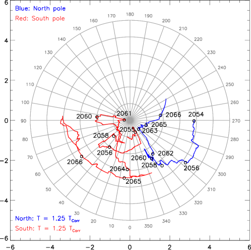
Figure 2: The evolution of the location of the Sun’s magnetic poles in a reference frame corotating with respect to the polar cap. North and south poles are drawn in blue and red, respectively. The concentric circles mark colatitudes from the heliographic pole in 1 degree steps. In the upper panel, the pole path is derived from the parameters displayed in Fig. 1. The rotational period that eliminates the average longitudinal drift of the north pole is 34.09 days. The lower panel shows the same evolution based on a surface flux transport simulation and a current sheet source surface extrapolation, in black. The rotational period of the nonaxisymmetric field was found in the simulation to be 28.67 days. The red and blue lines correspond to the model that includes artificial sunspots as discussed in the text.

When the surface field only varies slowly, the time dependence of the intercept $-v/u$ will be dominated by the Sun’s rotation. The intercept value should then oscillate with the Sun’s rotation frequency and with an amplitude that corresponds to the colatitude of the pole’s position. Its longitude is related to the phase of this oscillation: at the time when the intercept parameter is zero and rising, the pole is tilted towards Earth. To lowest order, this is what we observe in the recordings of the intercept $-v/u$ in Figs. 1a and b. Smooth changes in amplitude and phase indicate gentle motions of the pole (secular variation), and rapid changes allude to a rapid reorganization of the polar and probably of the whole coronal field. For these latter instances, our determination of the pole position is not rigorously valid. For the time period studied, the intercept parameter showed a mean period of $34.09$ days, and the location of the poles derived from an instantaneous oscillation amplitude and phase is shown in the upper panel of Fig. 2.

Similarly, the time variation of the slope parameter displays an oscillation with nearly twice the solar rotation frequency with a mean offset (see Fig. 1 c and d). Again for a stationary field, the minima and maxima of this oscillation are related to the minimum and maximum opening factors of the coronal pole field. To lowest approximation, these opening factors are defined in two orthogonal magnetically meridional planes that, except for a tilt of the magnetic pole towards or away from the observer, come close to the observer’s plane of the sky at times when the slope parameter assumes a maximum or a minimum.

2.3 Surface flux transport modeling and current sheet source surface model

As mentioned in the introduction, as an illustrative application of the method, we compare the observations with the magnetic field derived from surface flux transport simulations and a current sheet source surface extrapolation at each time step. For simplicity we used the results described in detail in (Jiang et al., 2010) and references therein. The source term for these simulations is based on the recorded sunspot records (again see Jiang et al., 2010, for details). Since the observations were taken during activity minima, relatively few sunspots were recorded for this period. From this model we extracted the field orientation at $1.19$ R_⊙ and on the plane of the sky. Similar to the processing of the plume orientations, the projected field orientations were transformed into cylindrical coordinates $(r,\phi)$ with respect to the solar disk center and subsequently processed by the Hough-wavelet transform. The resulting time series for the same time period covered by the observations is shown in Fig. 3. The solar rotation period derived from the simulated data was 28.67 days. To test how the magnetic pole location is sensitive to the emergence of sunspots, we artificially introduce a sunspot group at 2064 Carrington rotation. Two cases of sunspots are considered with different strengths and with same location. Their respective magnetograms are shown in Fig. 4, where we can see that the artificial sunspot groups are comparable to the other groups that were present at that time. The magnetic pole location and the opening factor are calculated and shown in Fig. 3. The location of the poles is derived and shown in Fig. 2 (bottom panel).

3 Discussion

The evolution of the magnetic poles position in the simulated case (bottom panel of Fig. 2, in black) is particularly simple: the poles rotate at a rate of 28.67 days and slowly drift towards the rotational pole (especially apparent in the southern hemisphere). This simple evolution reflects that no sunspots emerged during this time and so that no newly emerged flux were included for this time period in the simulation. The slow drift of the magnetic pole towards the rotational pole is due to the decay of a previously existing non-axisymmetric field as it is dispersed over all longitudes by differential rotation. When artificial sunspot groups are included in the simulation, the results show a clear change in the $-u/v$ parameter in Fig. 3 and in the magnetic pole locations in Fig. 2, which demonstrates that the magnetic pole location is sensitive to the flux emergence anywhere on the solar surface.

The evolution of the magnetic pole derived from the plume observations is more complicated. First, the the rotational period of 28.67 days is only a mean value, and there are times when the pole rotates faster and times when it rotates slower. This, in part, reflects that the rotation rate of magnetic fields do vary in time (Singh & Prabhu, 1985). Second, there is a more erratic behavior than in the simulations, with abrupt changes in the latitude of the poles. This directly reflects the amplitude changes of the oscillation of the intercept $-v/u$ seen in the left hand panels of Fig. 1. As in Wang et al. (1997), these changes in the coronal magnetic field are the result of small-scale flux emergences, which modifies the global magnetic field of the entire corona within an Alfvén transit time scale. An examination of SOLIS magnetograms covering this period showed, as expected, several small-scale flux emergence events that did not produce sunspots and therefore were not included in the surface flux transport simulations. This explains why the model intercept parameter $-v/u$ has a much cleaner periodic signal than the one based on the observations. On the other hand, it demonstrates the sensitivity of the parameters derived here to the structure of the coronal field.

Newly emerging flux, wherever it occurs on the Sun, produces a signature in the coronal magnetic field Wang et al. (1997) and, in particular, in the orientation of the polar plumes. Presently, the imaging of flux emergence on the far side of the Sun is made possible by complex inversion calculations of front-side helioseismology data (Lindsey & Braun, 2000). Although not pursued in this paper, our study suggests that a continuous monitoring of the orientation of polar plumes might improve our capability of far-side imaging of flux emergence.

The other parameters we measured were the opening factors. Their average corresponds to the mean slope parameter $<u>$, which reflects how much the polar field spreads out with distance from the solar surface. This parameter is about 50% larger in our observations than in the simulations. This indicates that the observed polar fields expand more rapidly from the photosphere than our simulations predict. A possible explanation for the discrepancy is a higher concentration of the photospheric field towards the poles of the Sun. The enhanced concentration suggests that the meridional velocity on the Sun is more efficient in convecting the magnetic field to the (rotational) poles than assumed in our flux transport simulations. These velocities are indeed poorly constrained by observations and in the flux transport simulations used here (Jiang et al., 2010). The meridional flow was simply assumed to vanish at 15 degrees from the poles. In this regard the observed average opening factor provides a sensitive constraint on the meridional flow near the poles where it is difficult to measure.

4 Conclusion and summary

We have carefully characterized the orientation of polar plumes and derived the time-dependent locations of the north and south magnetic poles. By comparing these results against surface flux transport simulations coupled with current sheet source surface models, we found that these properties are sensitive to the global magnetic field configuration, so are potentially useful in both understanding how the large-scale field reorganizes after flux emergence, and constraining the properties of flux emergence on the far side of the Sun. The average opening factor of the polar fields is suggested as a constraint on the strength of the near-polar meridional flow, which should be considered in future studies.

Our study supplements the earlier work of Wang et al. (1997), who used the orientation of streamers above the coronal belt to monitor reconfigurations of the coronal magnetic field. Using the orientation of plumes instead has the disadvantage that they are only observed during the solar activity minimum. Since flux emergence events occur most often at low and middle latitudes, the polar cap field is modified less by these distant sources, and the polar cap field sees more of an integral effect rather than local emergences. Definite advantages of our approach is that it is readily automated, it is continuously sensitive to all longitudes, and it can distinguish between temporal and spatial changes.

(a)

(b)

(c)

(d)

Figure 1: Time series of the intercept $-v/u$ (a and b) and the slope parameter $u$ (c and d) calculated for the north and south poles from data of EUVI A (in red), EUVI B (in blue), and EIT (in green) in the wavelength of 171 Å. The contributions of the different instruments are indicated by different colors. As explained in the text, the intercept is proportional to the projected heliographic colatitude $\tilde{\vartheta}_{c}$ of the magnetic pole location. The slope is a measure of the projected opening factor $f_{c}$ of the polar magnetic field at the respective pole (see labeling of the respective right ordinate axes).

Figure 3: Time series of the intercept $-v/u$ (upper panel) and the opening factor parameter $u$ (bottom panel) as in fig. 1 but calculated from the surface flux transport/current sheet source surface model (in black). The blue and red curves are the results from the model with extra sunspot groups corresponding to the synoptic magnetograms in Fig. 4, upper and middle panels, respectively. We only display the results for the northern hemisphere here.

Figure 4: Original synoptic magnetograms (bottom row) and two simulated magnetograms (top and central rows) with artificial sunspots of different strength. The left panels show the magnetograms with the sunspots at the time of their emergence, the right panels the magnetograms 54 days after emergence.