A Long XMM-Newton Observation of An Extreme Narrow Line Seyfert 1: PG 1244+026

Abstract

We explore the origin of the strong soft X-ray excess in Narrow Line Seyfert 1 galaxies using spectral-timing information from a 120ks XMM-Newton observation of PG 1244+026. Spectral fitting alone cannot distinguish between a true additional soft X-ray continuum component and strongly relativistically smeared reflection, but both models also require a separate soft blackbody component. This is most likely intrinsic emission from the disc extending into the lowest energy X-ray bandpass. The RMS spectra on short timescales (200-5000s) contain both (non-disk) soft excess and power law emission. However, the spectrum of the variability on these timescales correlated with the 4-10 keV lightcurve contains only the power law. Together these show that there is fast variability of the soft excess which is independent of the 4-10 keV variability. This is inconsistent with a single reflection component making the soft X-ray excess as this necessarily produces correlated variability in the 4-10 keV bandpass. Instead, the RMS and covariance spectra are consistent with an additional cool Comptonisation component which does not contribute to the spectrum above 2 keV.

1 Introduction

The spectral energy distribution (SED) of Active Galactic Nuclei (AGN) is powered by a mass accretion rate, $\dot{M}$, onto a central super-massive black hole of mass $M\sim 10^{6-9}M_{\odot}$. To the first-order approximation, as seen in the stellar mass black hole binaries, the state of the accretion flow is determined by $L/L_{Edd}$, where $L=\eta\dot{M}c^{2}$, $\eta$ is the efficiency set by black hole spin and the nature of the accretion flow, and $L_{Edd}=1.3\times 10^{38}M$ is the Eddington limit.

The highest Eddington ratio accretion flows, with $L/L_{Edd}\sim 1$, are found in the subset of broad line AGN known as Narrow-Line Seyfert 1s (NLS1s, e.g. Leighly 1999) which have permitted line widths only slightly broader than those of their forbidden lines (Osterbrock & Pogge 1985, Boroson & Green 1992), indicating relatively low black hole masses ($10^{6-7}M_{\odot}$: Boroson 2002). This combination of properties means that their accretion disc spectra should peak in the EUV/soft X-ray bandpass rather than the far UV peak expected for more typical Broad Line Seyfert 1 (BLS1)/QSOs which have $10^{8}M_{\odot}$, $L/L_{Edd}\sim 0.1$.

However, it has long been known that the spectra of AGN are more complex than expected from simple disc models. Standard QSO template spectra show substantial hard and soft X-ray emission as well as a ‘big blue bump’ from a standard disc (Elvis et al. 1994; Richards et al 2006). There is a power law which dominates in the 2-10 keV bandpass, and a soft X-ray excess over the low energy extrapolation of the power law emission which appears to be ubiquitous in all AGN. The power law ‘coronal’ emission is commonly seen also in black hole binaries (BHB), but the soft X-ray excess has no clear counterpart in the stellar mass systems. This could be a true additional continuum component seen only in AGN (Laor et al. 1997; Magdziarz et al. 1998; Gierliński & Done 2004), but the characteristic temperature of this component remains remarkably stable across objects of very different mass (Czerny et al. 2003; Gierliński & Done 2004), making this solution fine-tuned. The only current alternative model in the literature is that the soft excess instead arises as result of reflection and reprocessing from partially ionised material (Crummy et al. 2006; Walton et al. 2013). The decrease in opacity in this material below the Oxygen K and iron L edges at $\sim 0.7$ keV give a physical reason for the fixed energy of this feature. However, this requires similar fine tuning of the ionisation state of the reflecting material in order to always be dominated by the opacity at $\sim 0.7$ keV (Done & Nayakshin 2007). Also, the strong soft X-ray lines predicted by this model are not seen in the data, requiring extreme relativistic effects (high spin and highly centrally concentrated illumination) to smear these into a pseudo-continuum (Crummy et al. 2006; Walton et al. 2013).

These two very different ideas for the origin of the soft X-ray excess can be tested via variability. In the simplest reflection interpretation, both soft and hard X-rays are connected together by a single, partially ionised reflection component. Instead, if the soft X-ray excess is a true additional continuum component, this does not extend into the hard X-ray band and the soft and hard X-rays are decoupled. Previous work has addressed this via a range of different techniques mostly aimed at separating the spectrum into constant and variable components. In particular, the variable component can be quantified by calculating the excess variance in each (binned) energy channel (Edelson et al. 2002). These RMS spectra reveal a bewildering range of shapes (e.g. the compilation of Gierliński & Done 2006). These appear to be correlated with complexity of the X-ray spectra. The RMS spectra become more uniform after excluding NLS1 which show deep X-ray minima (these are the spectra which can be interpreted as being dominated by extreme relativistic reflection: Gallo 2006), and all objects where there is a strong warm absorber. Then, the remaining ‘simple’ AGN show RMS spectra where the low energy variability is strongly suppressed. These are consistent with a two component spectrum, where there is a stable soft component dominating at low energies, and a variable power law which dominates at high energies. This is seen in both NLS1 (Middleton et al. 2009; Jin et al. 2009) and BLS1 (Mehdipour et al. 2011; Noda et al. 2011; 2013).

Here we use an archetypal ‘simple’ NLS1 PG 1244+026 to further test these ideas on the origin of the soft X-ray excess and the shape of the SED. PG 1244+026 was selected by Jin et al. (2012a) (hereafter: J12a) as one of the brightest un-obscured Type 1 AGN with both XMM-Newton and SDSS spectra. From an analysis of optical spectra, PG 1244+026 can also be seen to have the narrowest H$\beta$ line (830 km s^-1) and the fourth smallest H$\beta$ equivalent width (41Å) of all of the PG quasars (Boroson & Green 1992). Previous X-ray observations of this source with ASCA revealed possible complexity around oxygen/iron L shell energies (Fiore et al. 1998; Ballantyne, Iwasawa & Fabian 2001), but the data were limited. Here we report on a new 120ks XMM-Newton observation which allows us to study the spectrum and variability of the source in detail.

This paper is organized as follows. We first describe the data quality and our data reduction procedure for this new XMM-Newton observation. Then in section 3 we try various models to fit the 0.3-10 keV spectra and report the results. Section 4 will focus on the variability of PG 1244+026, especially the light-curve, power spectral density (PSD) and the frequency-differentiated RMS spectra. In section 5, we will present the frequency-dependent covariance spectra and discuss their properties. In section 6, we will discuss issues such as broadband SED and black hole mass. The summary and conclusions are in Section 7.

Table 1: The model expression in xspec v12.7.1 for the four spectral fitting methods in Figure 1.

Model Name	Model Expression in xspec v12.7.1	seed photons
COMP-BBODY	CONSTANT*WABS*ZWABS*( BBODY + NTHCOMP + COMPTT + KDBLUR*PEXMON )	$kT_{bb}$ in bbody for comptt and nthcomp
COMP-COMPTT	CONSTANT*WABS*ZWABS*( BBODY + NTHCOMP + COMPTT + KDBLUR*PEXMON )	$kT_{e}$ in comptt for nthcomp
REFL	CONSTANT*WABS*ZWABS*( BBODY + NTHCOMP + KDBLUR*RFXCONV*NTHCOMP )	$kT_{bb}$ in bbody for nthcomp
IONPCF	CONSTANT*WABS*ZWABS*ZXIPCF*( BBODY + NTHCOMP )	$kT_{bb}$ in bbody for nthcomp

Figure 1: Four methods of X-ray spectral fitting for PG 1244+026. In each panel, black, blue and orange points are the spectra from EPIC PN, MOS1, and MOS2 respectively. Model components are the blackbody (red solid line) and intrinsic coronal emission (black dashed line). In Panel-a and b, the dash-dotted line is the soft excess described by Comptonisation, while the dotted line is the neutral reflection. In Panel-a, the seed photons for the high temperature Comptonisation are from the blackbody component, while in Panel-b they are from the soft X-ray Comptonisation component. In Panel-c, the dotted line is the smeared, ionised reflection component. In Panel-d, the dotted line is the fraction of power-law component after absorption by the partial-covering material. The data/model ratio is also plotted below each panel.

2 Data Reduction

PG 1244+026 was observed for $\sim$123 ks with the XMM-Newton satellite on the Christmas Day (Dec. 25th) 2011 (OBS ID: 0675320101). All three EPIC cameras were in small window mode to avoid the photon pile-up effect. We used SAS v12.0.1 and the latest calibration files, and followed the standard procedures to reduce the data. The entire observation period is free of high background flares, therefore the resulting good exposure time is $\sim$86 ks for the PN (due to the 71% live time in PN small window mode) and $\sim$120 ks for MOS (97.5% live time in MOS small window mode). We chose the source extraction region to be a circular region of radius 45″for each EPIC camera. For the PN, the background region was chosen to be a circle of radius 15″ as far as possible from the source while remaining on the same CCD chip. However, for the MOS cameras, the background region was taken from a different CCD chip as the central chip is fully occupied by the PSF of the source. The total source count rates are 11 ct s^-1, 2.2 ct s^-1 and 2.2 ct s^-1 for PN, MOS1 and MOS2 respectively, which are all well below the threshold count rates of causing photon pile-up effect in the small window mode of each EPIC camera.

We selected data with PATTERN $\leq$ 12 for MOS1 and MOS2, and PATTERN $\leq$ 4 for pn. Spectra were extracted from source and background regions separately. The response matrices were produced using RMFGEN and ARFGEN. The areas of source and background were calculated using BACKSCALE. Source spectra were rebinned by GRPPHA with a minimum of 25 counts per bin. All spectral fittings were performed in xspec v12.7.1 (Arnaud 1996). Lightcurves were also extracted from both source and background regions. Then the background lightcurve was subtracted from the source lightcurve using LCMATH in FTOOLS. Note that the mean background count rate within 0.3-10 keV is less than 0.3% of source count rate for every EPIC camera, and less than 20% even at $\sim$ 10 keV.

We also used the pipeline RGS order spectrum to check for narrow atomic features, grouped to a minimum of 10 counts/bin so that $\chi^{2}$ fitting is appropriate.

The OM UVW2, UVM2, UVW1, U, V band filters were used during the observation period, with 5 exposures in every filter, each exposure lasted 4600 seconds. We searched the merged OM source list file to find the count rate in each filter associated with the source, and pasted this into the OM data file template ‘om_filter_default.pi’ for use with the ‘canned’ response files in spectral fitting (see Section 6.2). We also extracted high resolution lightcurves from individual exposure files, combined and rebinned to 100s (see Section 4).

3 Time-averaged X-ray Spectral Modeling

We assume that the 0.3-10 keV spectrum contains an intrinsic coronal component which dominates the 2-10 keV bandpass. We also assume that there can be a contribution from the accretion disc itself, as the low mass, high mass accretion rate of NLS1 such as PG 1244+026 means that the disc can extend up to the soft X-ray bandpass (Done et al 2012: hereafter D12). We assume this disc emission above 0.3 keV can be approximated as a blackbody (bbody in xspec). The existence of a soft component close to the X-ray bandpass means that the coronal emission is not likely to remain as an unbroken power law at soft energies. If the disc or soft X-ray excess is the source of seed photons then the downturn in the Comptonised continuum is close to or within the observed soft X-ray bandpass. We use the Comptonisation model nthcomp in xspec (Zdziarski et al. 1996) so that this low energy turn-down is treated correctly.

We then include additional model components in order to describe the soft X-ray excess and remaining spectral features. We assume that all components are absorbed by the Galactic column of $N_{H}=1.87\times 10^{20}$ cm^-2 (Kalberla et al. 2005), but include an additional column of neutral absorption intrinsic to PG 1244+026 as a free parameter (zwabs with $z=0.048$). We assume an inclination of $30^{\circ}$ for all reflection fits, as is probably appropriate for a type 1 AGN. The total model is multiplied by a constant to account for the slight difference in the normalization between the EPIC PN, MOS1 and MOS2 spectra (it was fixed at unity for the PN).

The models are discussed in detail below, with results plotted in Figure 2 and best-fit parameters listed in Table 2.

3.1 Comptonisation

3.1.1 Seed photons from the disc (comp-bbody)

The blackbody and coronal emission alone give an unacceptable fit, with $\chi^{2}_{\nu}=3969/1805$. Including a cool, optically thick Comptonisation component (COMPTT model in xspec: Titarchuk 1994) with seed photon temperature tied to the blackbody temperature reduces this to $2312/1802$, showing clearly that the soft excess is broader than a single blackbody. This continuum model has $\Gamma=2.32\pm 0.02$. Adding neutral, relativistically smeared reflection (kdblur*pexmon Laor 1991, recoded as a convolution model, Nandra et al. 2007) gives a significantly better fit with $\chi^{2}_{\nu}=2261/1800$ for $\Omega/2\pi\sim 1.5$ for solar abundance, and $R_{in}=16R_{g}$, steepening the intrinsic continuum to $\Gamma=2.50_{-0.02}^{+0.04}$.

The expression of the total model in xspec is listed in Table 1, along with best-fit free parameters listed in Table 2. The unfolded spectra are plotted in Figure 1a. The 2-10 keV photon index (hereafter: $\Gamma_{2-10keV}$) is 2.50, which is among the steepest hard X-ray slope in all NLS1s (e.g. Grupe 2004; Jin et al. 2012c). The temperature for the low temperature Comptonisation is 0.16 keV, similar to the $\sim$0.2 keV temperature seen for this component in all high mass accretion rate AGN (Czerny et al. 2003; Gierliński & Done 2004). The blackbody temperature is below the bandpass at 60 eV but the Wien tail from this is significantly detected in the data (removing the bbody increases $\chi^{2}_{\nu}$ to $2361/1802$).

3.1.2 Seed photons from Comptonisation (comp-comptt)

We then assume that the seed photons for the coronal Comptonisation component are from the comptt component, as appropriate for the geometry sketched in D12 where the soft excess represents incomplete thermalisation in the inner disc, and the corona is above the inner disc. This mainly increases the norm of both the blackbody and cool compton components as the higher seed photon temperature reduces the low energy coronal flux. We show this fit in Figure 1b, with best fit parameters in Table 2.

The neutral reflection in both fits is rather larger than expected for isotropic illumination. We caution that the lack of signal-to-noise at high energies means that the preference for a larger reflection fraction is probably driven by a preference for a steep power law in the 0.5-5 keV bandpass, and that this in turn is dependent on the detailed model assumed for the soft X-ray excess (single electron temperature, single optical depth, single seed photon temperature and seed photons with a Wien spectrum). Better high energy data is required to test how much reflection is really present in these data.

3.1.3 Iron L emission line

The models above are a good fit to the data, but there are significant residuals at iron L, as seen previously (Fiore et al. 1998). Including a Gaussian line gives $\chi^{2}_{\nu}=2129/1797$ (i.e. $\Delta\chi^{2}=132$ for 3 additional degrees of freedom) for a centroid energy of $0.92$ keV with intrinsic width of 80 eV (so the line is too broad to be seen in the RGS) and equivalent width of 12 eV. This line energy is consistent with iron L emission, suggesting the presence of ionised material, whereas the model here only includes neutral reflection. Hence we investigate the ionised reflection models as the origin of the soft X-ray excess.

3.2 Ionised Reflection (refl)

The fits above assumed that the soft excess was a true continuum component, but an ionised reflector also includes a strong rise at low energies due to the decrease in soft X-ray opacity of partially ionised material and should also include features from iron L and Oxygen emission (e.g. Fabian et al. 2009). We remove the comptt and pexmon components and allow both the soft X-ray excess and iron K$\alpha$ line to be fit by the same partially ionised reflector with super-solar iron abundance (e.g. as seen in 1H 0707-495, Fabian et al. 2009). We model this using rfxconv, which is based on the ionised reflection tables of Ross & Fabian (2005), recoded into a convolution model (Kolehmainen, Done & Diaz Trigo 2011). The associated atomic features are not seen in the data, so the model requires extreme relativistic smearing to match the observed, mostly smooth continuum form. We follow previous work and allow the emissivity to be a free parameter as well as $R_{in}$ (Crummy et al. 2006). This gives $\chi^{2}_{\nu}=2322/1802$, for an emissivity of $4$, $R_{in}=3R_{g}$, a 2x overabundance of iron and ionisation parameter of $\log\xi=3$, subtending a solid angle $\Omega/2\pi\sim 1.5$, where the requirement for a large solid angle is mainly driven by the soft X-ray excess.

This reflection dominated model for the soft X-ray excess gives a very different spectral decomposition around the iron K line than the comp-bbody and comp-comptt models. Here there is a substantial amount of partially ionised, strongly smeared reflection in the 4-10 keV spectrum, whereas before there was a smaller amount of neutral, moderately smeared reflection. However, the signal-to-noise in the high energy bandpass is not sufficient to distinguish between these two models.

Overall the fit is not as good as those derived above from allowing an additional soft excess component and a free iron L line, showing that a single ionised reflector is not able to simultaneously describe the shape of the soft excess, iron K alpha line and iron L line. Part of this may be because the low energy line emission in the ionised reflection models is predominantly Oxygen rather than iron L. However, the specifics of the line emission depend on the underlying thermal structure of the reflector. The Ross & Fabian (2005) models assume that the reflector has no net flux entering from below, whereas reflection from the disc would have an additional ionisation level from collisional processes as well as photo-ionisation.

3.3 Partially ionised, partial covering absorption: ionpcf

Another scenario to model the X-ray spectrum is partial-covering absorption by clumpy material along the line of sight (e.g. Miller et al. 2007; Tatum et al. 2012). If this material is structured in a wind then there can also be a contribution from scattering (e.g. Sim et al. 2010). Such material could also be partially ionized since it is directly illuminated by the central ionizing flux. We used xspec model zxipcf (Reeves et al. 2008) to multiply the intrinsic power law to produce the partially absorbed power law.

Adding a single partially ionised, partial covering component does not describe the data well, with $\chi^{2}_{\nu}=3777/1802$, mainly due to the failure of partial covering model to follow the curvature of the soft excess around 1 keV. The inferred power law index is extremely steep, with $\Gamma=3.6$, but the only clear atomic features predicted by the model are some iron K alpha absorption lines around 6.6 keV.

Including a second partial-covering component gives a better, but still not acceptable fit, with $\chi^{2}_{\nu}=3430/1801$ and the spectrum is still extremely steep, at $\Gamma=3.6$.

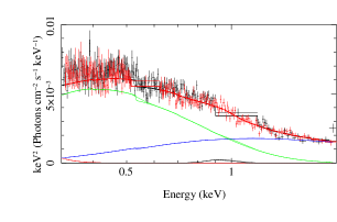
Figure 2: The RGS1 (black) and 2 (red) spectra, devolvolved using the best fit comp-comptt model (diskbb: red line, comptt: green line, nthcomp: blue line, gaussian: black line, see Section 3.1.3). This broad iron L line emission is consistent with the data, and there are no significant narrow absorption or emission features.

Table 2: The best-fit value of the parameters in the four spectral fitting in Figure 1. The upper and lower limits give the 90% confidence range.

Model	Component	Parameter	Value
COMP	$\chi^{2}_{\nu}~{}=~{}2261/1800~{}=~{}1.26$
:BBODY	ZWABS	NH (1022 $cm^{-2}$)	0 ${}^{+0.001}_{-0}$
	BBODY	kT (keV)	0.058$\pm 0.002$
	BBODY	norm	1.3$\pm 0.1\times 10^{-4}$
	NTHCOMP	$\Gamma$	2.50 ${}^{+0.04}_{-0.02}$
	NTHCOMP	kTseed (keV)	tied
	NTHCOMP	kTe (keV)	100 fixed
	NTHCOMP	norm	2.29$\pm 0.05\times 10^{-3}$
	COMPTT	kTseed (keV)	tied
	COMPTT	kT (keV)	0.160 $\pm 0.003$
	COMPTT	$\tau$	96 ${}_{-60}^{+100}$
	COMPTT	norm	0.072 ${}_{-0.004}^{+0.06}$
	KDBLUR	Rin ($R_{g}$)	16 ${}^{+9}_{-6}$
	PEXMON	Relrefl	-1.5 ${}^{+0.3}_{-0.2}$
COMP	$\chi^{2}_{\nu}~{}=~{}2263/1800~{}=~{}1.26$
:COMPTT	ZWABS	NH (1022 $cm^{-2}$)	0 ${}^{+0.001}_{-0}$
	BBODY	kT (keV)	0.062 ${}^{+0.001}_{-0.002}$
	BBODY	norm	1.8 ${}^{+0.1}_{-0.2}\times 10^{-4}$
	NTHCOMP	$\Gamma$	2.53 ${}^{+0.02}_{-0.03}$
	NTHCOMP	kTseed (keV)	tied to kTe
	NTHCOMP	norm	2.1 $\pm 0.1\times 10^{-3}$
	COMPTT	kTe (keV)	0.15 ${}^{+0.003}_{-0.003}$
	COMPTT	$\tau$	38 ${}^{+150}_{-20}$
	COMPTT	norm	0.16 $\pm 0.01$
	KDBLUR	Rin ($R_{g}$)	16 ${}^{+8}_{-6}$
	PEXMON	Relrefl	-1.76 ${}^{+0.32}_{-0.26}$
REFL	$\chi^{2}_{\nu}~{}=~{}2322/1802~{}=~{}1.29$
	ZWABS	NH (1022 $cm^{-2}$)	0.015 ${}^{+0.004}_{-0.003}$
	BBODY	kT (keV)	0.053 ${}^{+0.004}_{-0.004}$
	BBODY	norm	1.3 ${}^{+2.3}_{-0.3}\times 10^{-4}$
	NTHCOMP	$\Gamma$	2.58 ${}^{+0.01}_{-0.01}$
	NTHCOMP	norm	1.61 ${}^{+0.09}_{-0.07}\times 10^{-3}$
	KDBLUR	Index	3.97 ${}^{+0.22}_{-0.13}$
	KDBLUR	Rin ($R_{g}$)	3.04 ${}^{+0.08}_{-0.02}$
	RFXCONV	Relrefl	-1.52 ${}^{+0.14}_{-0.56}$
	RFXCONV	Feabund	1.95 ${}^{+0.11}_{-0.09}$
	RFXCONV	log$\xi$	3.06 ${}^{+0.02}_{-0.02}$
IONPCF	$\chi^{2}_{\nu}~{}=~{}3430/1801~{}=~{}1.91$
	ZWABS	NH (1022 $cm^{-2}$)	0.088 ${}^{+0.002}_{-0.001}$
	BBODY	kT (keV)	0.050 fixed
	BBODY	norm	$8.9\times 10^{-5}$ fixed
	NTHCOMP	$\Gamma$	3.61 ${}^{+0.01}_{-0.02}$
	NTHCOMP	norm	0.091 ${}^{+0.006}_{-0.010}$
	ZXIPCF	NH,1 (1022 $cm^{-2}$)	13 ${}^{+0.62}_{-0.39}$
	ZXIPCF	log$\xi_{1}$	0.83 ${}^{+0.12}_{-0.14}$
	ZXIPCF	fcover,1	0.80 ${}^{+0.002}_{-0.011}$

3.4 High resolution spectra

We fit the high resolution RGS data with the best fit comp-comptt model discussed in Section 3.1.2. All parameters were frozen at the best fit values given in Table 2, but a constant offset (best fit value of 0.92) was allowed, to take into account possible calibration differences between the gratings and CCDs. This gives a good fit, with $\chi^{2}_{\nu}=4268/4205$. We then include the iron L line, again fixed that seen in the CCD detectors, and find $\chi^{2}_{\nu}=4256/4205$, so this weak, broad feature is consistent with the grating spectra. Figure 2 shows the RGS data de-convolved with this model. It is clear that there are no narrow absorption features evident by eye. We quantify this fitting a warm absorber zxipcf, assumed to cover the entire source. We allow this to be outflowing to a maximum velocity of $0.1$ c. This model is only tabulated down to columns of $5\times 10^{20}$ cm^-2, but the fit pegs to this value, giving $\Delta\chi^{2}$ of $5$ worse than no absorption at all for $\log\xi=3$. The fit becomes progressively worse at lower ionisations, with $\Delta\chi^{2}$ increased to $15$ at $\log\xi=2.4$ and $110$ for $\log\xi=1.6$.

Thus it is clear that none of the curvature below 2 keV seen in the CCD spectra is due a classic ‘warm absorber’, though we note that the ionpcf fits in Section 3.3 (which model the complexity around the iron K$\alpha$ line by partial covering) do not predict any features below 2 keV.

3.5 Summary of spectral fits

The main question addressed in this paper is the origin of the soft X-ray excess, whether it is predominantly a separate soft continuum component, or extremely smeared reflection or due to the spectral curvature associated with complex absorption. These models are not necessarily mutually exclusive, nor are they the only models which can be envisaged. For example, we used neutral reflection in the models where the soft excess was fit by a separate components (comp-bbody and comp-comptt). The reflector could instead be ionised, giving some contribution to the soft X-ray excess, while there may be an additional true soft continuum which contributes to the refl or ionpcf fit. There could also be multiple reflectors (e.g Fabian et al 2002) or absorbers (e.g. Miller et al 2007). We do not explore these composite models further as we are concerned with the origin of the majority of the soft X-ray excess. The spectral fits alone rule out complex absorption as a major contributor to the soft X-ray excess, so in what follows we use variability to try to distinguish between a separate soft component and an extremely smeared reflection origin for the majority of the soft X-ray excess.

4 Lightcurve and Variability

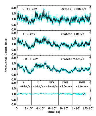
Figure 3: The 100s binned light-curves in each X-ray energy band and the five OM filters, divided by the mean count-rates given in the bracket. Error-bars are shown in cyan.

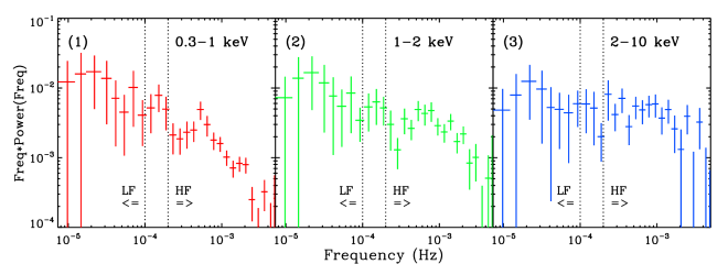
Figure 4: The power spectrum of each energy band after subtracting the Poisson counting noise, calculated by FTOOL task POWSPEC, rebinned as a geometrical series with geometrical step equal to 1.2.

4.1 Power spectra

Figure 3 shows the light-curves in both soft, medium and hard X-ray, together with the simultaneous optical/UV data from the OM. These is no significant variability in the optical/UV but the X-rays show fluctuations on all time-scales from tens to thousands of second, with subtle changes in the amount of variability with energy. We study this in more detail by taking the power spectral density (PSD).

Each X-ray light-curve shown in Figure 3 was a combination of three 100s-binned background subtracted light-curves from the three EPIC cameras separately. The FTOOL task LCMATH was used to perform this light-curve merging. Then FTOOL task POWSPEC was used to perform a DFT on each of these three light-curves to derive the periodogram, which is a realisation of the intrinsic continuous PSD (e.g. Vaughan et al. 2003). The norm parameter of POWSPEC was set to $-2$, such that white noise is subtracted and the remaining power integrates to give the excess variance in the lightcurve. These PSDs are plotted as $fP(f)$ in Figure 4.

These show differences between the PSD shapes at each energy, with the 2-10 keV bandpass showing more power at the highest frequencies than the lowest energy band. This is a common feature of NLS1 power spectra (e.g. M^cHardy et al. 2004). There is also some potential structure in the PSD of the 0.3-1 keV lightcurve (left panel in Figure 4) around ${\sim}5{\times}10^{-3}$Hz, possibly resembling the double Lorentzian fit to the PSD of Ark 564 (M^cHardy et al. 2007) though the statistical significance of this would require widespread simulations to assess, which are beyond the scope of this paper.

4.2 Frequency-dependent Fractional RMS Spectra

We have divided the 0.3-10 keV into different energy bands and explored their PSDs. But we can also divide the observed frequency range into bands, and explore the more detailed energy-dependence of the fractional variability for each frequency band, i.e. the RMS spectrum (e.g. Edelson et al. 2002; Markowitz, Edelson & Vaughan 2003; Vaughan et al. 2003).

There are two ways to calculate the RMS spectra in the literature. The most straightforward is where the light curve (length $T$, bin time $\Delta t$) is divided into $M$ segments. The excess variance in each segment is averaged together to give a measure of the RMS over a frequency range from $M/T$ to $1/(2\Delta t)$, with error given in Vaughan et al (2003). However, red noise leak can be an issue with this if there is substantial variability power at frequencies lower than $M/T$. We instead use the alternative approach, which calculates the RMS by integrating the power spectrum of the full lightcurve (from $1/T$ to $1/(2\Delta t)$) only over the frequency range of interest, as this suppresses red noise leak. We calculate errors following Poutanen, Zdziarski & Ibragimov (2008). This uses Poisson errors, so non-gaussianity of low counts is not an issue at high energy, but it is not clear how to treat a zero count bin. We choose the smallest energy bands which are compatible with not having more than 10% of the bins with zero counts.

We also tested whether the background subtraction would affect our calculation, especially at high energies above 4 keV where the count rate is low. We found the background count rate was only 10-20% of the source count rate in the 8-10 keV bin, and much less at lower energies. The background subtracted source RMS in the HF band is 0.13$\pm$0.02, not significantly different to the non-background subtracted HF RMS in this band of 0.14$\pm$0.02. Therefore, we conclude that our results were not affected by background subtraction.

The fractional RMS spectrum for the whole observed frequency band i.e. from $8\times 10^{-6}-5\times 10^{-3}$ Hz (123ks-200s) is shown as the black points in Figure 5. The total RMS spectrum is relatively flat, with a small dip at 3$\sim$4 keV. This is an unusual shape, as it is not similar to the 1-2 keV peaked shape seen in the extreme low state NLS1, which may indicate that the spectra are dominated by reflection (e.g. Fabian et al 2004), nor is it similar to the high state NLS1 (e.g. RE J1034+396) where the low energy variability is strongly suppressed, which may indicate that the soft excess is a separate component (Middleton et al. 2009; Jin et al. 2009).

However, RE J1034+396 showed different RMS at different frequencies (Middleton et al. 2009). We explore whether the same is true for PG 1244+026, by dividing the data into two frequency bands, i.e. low frequency ([$8\times 10^{-6}$Hz, $1\times 10^{-4}$Hz] or [10ks, 123ks], hereafter: LF, red points), and high frequency ([$2\times 10^{-4}$Hz, $5\times 10^{-3}$Hz] or [200s, 5ks], hereafter: HF, blue points). The RMS spectra for these bands are shown in Figure 5. It is clear that at LF, the soft X-rays are more variable than the hard X-rays; while the opposite is true at HF. This clearly shows the reason for the unusual total RMS spectrum, which is because it is the sum of two very different spectral behaviours at high and low frequencies.

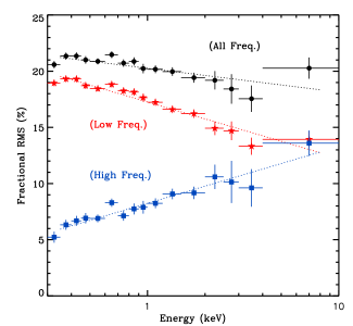
Figure 5: The fractional RMS spectrum for each frequency band. Dotted lines are simple linear fitting to every spectrum to highlight the spectral trend.

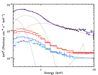
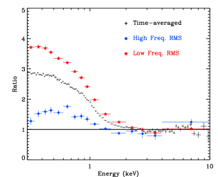
Figure 6: a) Comparison between the time-average spectrum (black) and RMS spectra for HF (blue) and LF (red), respectively. The black lines show the best fit model components to the time averaged spectrum, with blackbody, cool, optically thick Comptonisation, hot, optically thin Comptonisation and neutral reflection shown as the dotted lines. The blue and red solid lines show the total model scaled by 0.1 and 0.15 respectively to match the HF and LF power law. The dashed blue and red lines show the model assuming both blackbody and soft excess are further scaled by a factor 0.6 and 1.3 for HF and LF respectively. b) Ratio of each spectrum to its best fit 2-10 keV power law highlighting the changing strength of the soft X-ray excess with variability timescale.

4.3 Frequency-dependent Absolute RMS Spectra

We explore the frequency dependent spectral behaviour in more detail by multiplying the fractional RMS in each energy bin by the mean count rate in that bin to produce absolute RMS spectra. These can then be fit directly in xspec using the standard instrument response (e.g. Revnivtsev et al. 2006; Sobolewska & Życki 2006; Middleton et al. 2011). PN and MOS produced identical lightcurves, but they have different response files and slightly different spectral normalisation. Therefore we only used the mean count rate from the PN time-averaged spectrum to calculate the absolute RMS, and used the PN response file in xspec fitting.

We compare the absolute RMS spectra with the PN time-averaged spectrum in Figure 6a using the comp-comptt model from Section 3.1.2, multiplied by 0.1 and 0.15 (for HF and LF, respectively). Plainly, this over-predicts the soft X-ray variability in the HF and under-predicts it in the LF. Figure 6b illustrates this dependence of the soft X-ray excess on variability timescale by showing the ratio of each spectrum with the best fit 2-10 keV power law. The soft X-ray excess is much stronger relative to the power law emission in the low frequency variability spectrum than in the fast variability spectrum. This is as expected from the power spectral results (Figure 4), as these show that there is more variability in the hard band than the soft at high frequencies, and more variability in the soft band than the hard at low frequencies. The dashed lines in Figure 6a show the model assuming that the blackbody and soft excess are scaled by a factor 1.3 relative to the coronal emission in the LF (red dashed), and a factor 0.6 in the HF (blue dashed). This models the variability well, though the HF RMS are slightly over-predicted at the softest energies, perhaps indicating that the blackbody is not varying as strongly as the soft X-ray excess.

The alternative refl models (section 3.2) can also match these data, this time by changing the amount of ionised reflection (to $\Omega/2\pi\sim 2.5$ and $1$ for LF and HF respectively, compared to $1.5$ in the time averaged spectrum. These models give a slightly better match to the rise in the final HF RMS spectral bin between 4-10 keV (as discussed in Section 5.1), though we caution that the lack of statistics (in particular the number of bins with zero counts) may be an issue here.

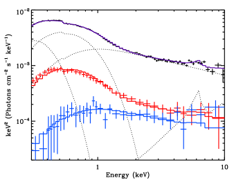
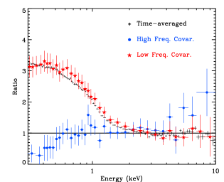
Figure 7: a) As for Figure 6 a and b, but with the 4-10 keV covariance spectra for HF (blue) and LF (red), respectively. The 4-10 keV HF covariance spectrum clearly shows no component of the soft X-ray excess or soft blackbody emission.

5 Frequency-dependent Covariance Spectra

The RMS spectrum shows the total variability at a specific frequency range in every energy bin, but the very limited signal-to-noise at high energies prevented us from reducing the width of energy bin further in the RMS spectrum. One way to increase the spectral resolution of variability is to look only for the correlated variability via the ‘covariance spectrum’, a technique developed by Wilkinson & Uttley (2009). A ‘reference band’ can be chosen to give a high signal-to-noise lightcurve and cross-correlated with the lightcurve in each individual band. The correlated variability in each energy band has much smaller error bars as it removes the uncorrelated white noise variance. This makes it a more sensitive technique so it can be used to explore the variability at higher energies. It also has obvious advantages in that it explicitly pulls out the correlated variability. Both the power law and its reflection contribute to the 0.3-1 keV and 4-10 keV bands if reflection makes the soft X-ray excess, whereas these energies are connected only by the power law in the Comptonisation models.

We derive the covariance spectrum for the HF and LF frequency ranges again using the power spectra. We used a DFT to transform the light-curve into a periodogram; then kept a specific frequency range while letting all the power outside this range be zero; then used the inverse DFT to transform the band-limited periodogram back to a new light-curve. This new light-curve has the same mean count-rate as the original light-curve, but only contains variability over the chosen frequency range. We applied the frequency filter to the light-curve in every energy bin, and then followed the procedure in Wilkinson & Uttley (2009) to derive the covariance spectrum without dividing the light-curve into small segments. The resultant covariance spectrum is only for the specific frequency range, and so is frequency-dependent. When the energy bin for which the covariance is being calculated is within the reference band, we recalculate the reference band lightcurve excluding that channel so that Poisson errors are never included in the correlated signal.

This should also pull out any correlated variability which has a short (with respect to the binning) time lag/lead. Recent studies of the similar mass and mass accretion rate object 1H 0707-495 have shown a lag of 30s of the soft band behind the high energy variation at high frequencies (Fabian et al. 2009). This is within our bin time of 100s so we would include any component which lags or leads on this timescale in our covariance spectrum.

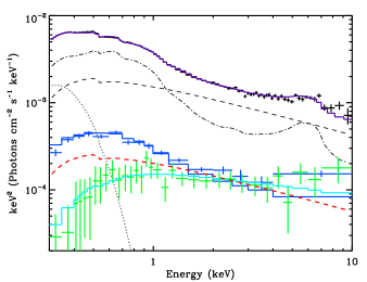
Figure 8: Comparison between the time-average spectrum (black), HF RMS spectrum (blue) and the HF 4-10 keV covariance spectrum (green). The time-averaged spectrum is shown decomposed with the refl model. The HF RMS spectrum does show variability in the soft X-ray excess but the lack of this in the HF covariance component shows that none of this fast variability in the soft excess can correlate with the 4-10 keV flux changes, ruling out the refl model. Furthermore, the turndown in the covariance spectrum below 1 keV clearly shows that the seed photons for the continuum are at soft excess energies rather than from the disc component as assumed in the refl model (dashed red line).

5.1 High Energy Covariance: 4-10 keV reference band

We choose 4-10 keV as the reference band, as this is the one where the Comptonisation and reflection models for the soft X-ray excess show most difference. This band contains both the soft excess component (ionised, blurred reflection) and the continuum in the refl model, but does not contain any of the soft X-ray excess in the comp-comptt model.

Figure 7(a) shows the LF (red) and HF (blue) covariance spectra, compared to the time averaged spectrum, while (b) shows the ratio of each spectrum to its best fit 2-10 keV power law. The LF covariance spectrum is very similar to the time averaged spectrum, but the HF covariance is completely different, lacking all soft excess and blackbody components. Thus on timescales of 5000-200s none of the soft excess variability seen in the HF RMS spectrum correlates with the hard X-ray lightcurve.

We show this in more detail by showing the HF RMS (blue) and covariance (green) spectra together with the time averaged spectrum (black) in Figure 8. There is clearly more soft variability in the RMS spectrum than in the covariance spectrum. Thus there is some fast variability in the soft excess (as shown by the power spectra), but this is uncorrelated with the fast variability in hard X-rays (or correlated with a lag/lead much longer than the 100s bin time). The black lines show the best fit reflection model to the time averaged spectrum. The blue solid line shows the best fit model of these components to the HF RMS spectrum, resulting in the blackbody normalisation going to zero, while the amount of reflection reduces to $\Omega/\pi\sim 1$ (as discussed in Section 4.3). The red dashed line shows a similar fit to the HF covariance spectrum (green). Even with the blackbody and reflection normalisations set to zero, the intrinsic power law in the reflection fit is too steep to match the correlated spectrum. The cyan solid line shows instead the coronal ‘power law’ emission from the Comptonisation model for the soft X-ray excess (comp-comptt). Plainly this is a much better fit to the slope of the covariance spectrum, as well as having the downturn for seed photons at the correct energy assuming that these are from the soft excess.

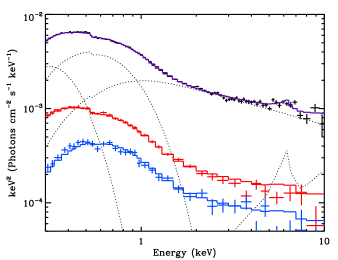
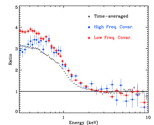
Figure 9: As in Fig 6a and b but using 0.3-1 keV as the reference energy band. a) The blue and red solid lines show the total model scaled by 0.08 and 0.16 respectively to match the HF and LF power law, except that the hot, optically thin Comptonisation was further scaled down by 0.85 in both HF and LF models, and blackbody was removed from the HF model. b) the ratio of the spectra to their 2-10 keV best fit power law. The LF and HF components are very similar except for the drop in HF covariance at the lowest energies, indicating the physical reality of the additional blackbody component.

The key issue is the difference between the RMS and covariance spectra shows that there is variability in the soft X-ray excess which is not correlated with variability in the 4-10 keV bandpass. Yet in reflection models, the soft X-ray excess variability contributes to variability in the 4-10 keV bandpass so these cannot be uncorrelated. Another difference is that the intrinsic ‘power law spectrum’ in the reflection model is significantly steeper than in the Comptonisation model. Yet the covariance spectrum alone fit to a hot (temperature fixed at 100 keV) Comptonisation component gives $\Gamma=2.25\pm 0.2$, significantly flatter than the $\Gamma=2.58\pm 0.01$ derived from the time averaged spectrum reflection fit, but consistent with the overall (including reflection) spectral index of $\Gamma=2.32\pm 0.02$ seen in the Comptonisation model. The seed photon energy of $0.13\pm 0.04$ keV is also consistent with the soft excess being the source of seed photons for the hot corona, and not with the lower temperature disc.

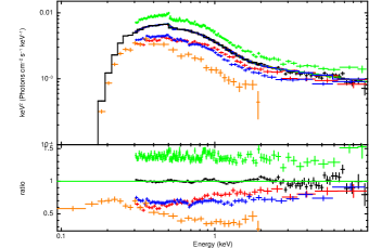
Figure 10: The short and long term X-ray variability. The black spectrum is the time-averaged XMM-Newton EPIC PN spectrum from the 2011 observation, with the blue and green spectra extracted from all time intervals of count rates ${\leq}$0.75 and ${\geq}$1.25 of the mean count rate separately. The red spectrum is the time-averaged XMM-Newton EPIC PN data from the 2001 observation. The orange spectrum is from the 1991 ROSAT PSPCB observation. The lower panel shows the ratio between these spectra and the best-fit Comptonisation model to the black spectrum.

5.2 Low energy covariance: 0.3-1 keV reference band

The difference between the HF RMS and 4-10 keV HF covariance spectra shows that the soft excess varies independently from the high energy continuum. Figure 9(a) shows the HF and LF covariance spectra extracted with a reference band 0.3-1 keV to focus on this variability, while (b) shows these as a ratio to the (scaled) high energy power law emission. The difference between the HF and LF covariance spectra is much less dramatic using the low energy lightcurve as the reference band. The only significant difference between the LF and HF 0.3-1 keV covariance spectra are that the HF covariance spectrum dips at the lowest energies, indicating that there is a separate component, described here as an additional blackbody, which contributes only below 0.5 keV.

We fit the covariance spectra using the comp-comptt model. Fig 9(a) shows this best fit time average model scaled by 0.16 (LF, red) and 0.08 (HF, blue), respectively, but with the blackbody component removed from the HF model. This matches the downturn seen in the HF covariance spectrum at the lowest energies, showing clearly that the soft X-rays are composed of two components, in addition to the extrapolated high energy emission. This softest emission component is most plausibly the disc for this low mass, high mass accretion rate NLS1 (see section 6).

Table 3: Parameters of the four spectra in Figure 10. obs1: pn spectrum on 2001; obs2: pn spectrum on 2011; obs2-l: pn spectrum from time-intervals with count rates $\leq$0.75$\bar{x}$; obs2-h: pn spectrum from time-intervals with count rates $\geq$1.25$\bar{x}$. $\Gamma_{0.5-2}$: the 0.5-2 keV power law photon index. $R_{0.5keV}$: the data/model ratio at 0.5 keV, the model is the extrapolation of the best-fit power law to the 2-10 keV spectrum of obs2. R_f-10keV: the 2-10 keV flux ratio between other spectra and obs2, the absolute 2-10 keV flux for obs2 is $3.07{\times}10^{-12}~{}ergs~{}cm^{-2}~{}s^{-1}$; HR: hardness-ratio defined as (H-S)/(H+S), where S is the photon number in 0.5-2 keV and H is the photon number in 2-10 keV.

Spec	$\Gamma_{2-10}$	$\Gamma_{0.5-2}$	R0.5keV	Rf2-10	HR
obs1	2.45${}^{+0.12}_{-0.12}$	2.95${}^{+0.64}_{-0.57}$	2.20$\pm$0.12	0.79	-0.840
obs2	2.37${}^{+0.03}_{-0.03}$	3.16${}^{+0.14}_{-0.14}$	2.64$\pm$0.03	1	-0.853
obs2-l	2.21${}^{+0.09}_{-0.08}$	3.15${}^{+0.56}_{-0.50}$	2.40$\pm$0.11	0.72	-0.847
obs2-h	2.39${}^{+0.06}_{-0.06}$	3.18${}^{+0.33}_{-0.31}$	2.92$\pm$0.08	1.29	-0.863

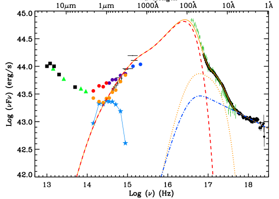
Figure 11: The broadband SED of PG 2144+026, corrected for both Galactic and intrinsic reddening/extinction. Data includes (from high to low energy) XMM-Newton EPIC spectra (black), ROSAT PSPCB spectrum (green) spectrum above 100Å); GALEX photometry (blue circles); XMM-Newton OM photometry (black), SDSS fiber spectrum (black) SDSS ugriz photometry: PSF magnitude (purple circles), Petrosian magnitude (orange circles) and their discrepancy (cyan stars); UKIDSS YJHK photometry: Aper-3 magnitude (red circles), Petrosian magnitude (red circles) and their discrepancy (cyan stars); WISE 4-band photometry (green triangles); Spitzer IRS continuum (black squares). Orange solid line is the best-fit model to the XMM-Newton EPIC spectra, OM points, ROSAT spectrum and SDSS spectrum, using optxagnf model in xspec which includes accretion disc (red dashed line), low temperature Comptonisation (orange dotted line) and high temperature Comptonisation (blue dash-dotted line). Note that the cyan stars form a typical spectral shape of host galaxy contamination.

6 Multi-wavelength spectral energy distribution

In this section, we construct the multiwavelength SED from non-simultaneous observations. Hence we first have to assess the effect of long term variability.

6.1 Long term variability

The XMM-Newton observation has provided high quality simultaneous data in both X-ray and optical/UV for PG 2144+026. We also made use of the SDSS spectrum to help define the optical continuum. Although there was a 10 year interval between the SDSS (obs-date: 2001-04-25) and XMM-Newton observation, we found that they were fairly consistent with the OM optical data. There is a previous XMM-Newton dataset taken in 2001-06-17 (60ks of good exposure in every EPIC camera), close in time to the SDSS data, but the OM was switched off for this observation.

Instead we extract the X-ray data from the 2001 XMM-Newton observation (blue: Fig 10) and compare this with the time-averaged X-ray spectra from our 2011 XMM-Newton data (black: Fig 10). While the flux at 10 keV remains almost the same, the flux below 0.5 keV is lower by a factor 0.75 in the 2001 observation. We compare this to the short timescale variability seen within our single observation by accumulating a high flux spectrum (green: where the flux is more than 25% higher than the mean) and a low flux spectrum (red: where the flux is more than 25% lower than the mean). Plainly the blue and red spectra are quite similar, so the long timescale variability over decades is of similar amplitude to the short timescale variability seen within a single observation. Hence it seems likely that there is no dramatic change in the SED over the timescales spanned by the multi-wavelength data. Details of these X-ray spectra are given in Table 3.

There is also archival data from ROSAT PSPCB which can be used to extend the X-ray spectrum down to 0.1-0.2 keV. This was taken on 1991-12-22. We extracted this using XSELECT v2.4b and followed the standard procedure to reduce the data and extract the source and background spectrum. This is also shown on the long term X-ray variability figure, where it is a factor 0.44 below the time averaged 2011 XMM-Newton data although its shape is similar in the 0.3-2 keV region of overlapping bandpass.

Table 4: The parameters of the optxagnf model in Fig 12. nH_int is the best-fit intrinsic extinction; $z$ is the redshift; R_cor is the coronal radius; T_e is the electron temperature for the soft X-ray Comptonisation; $\tau$ is the optical depth of the low temperature electron population; F_pl is the fraction of luminosity contained in the hard X-ray Comptonisation compared to the total coronal luminosity. FWHM was measured from the H$\beta$ line profile after subtracting the narrow component.

Name	nHint	$z$	$\Gamma_{2-10keV}$	Lbol	MBH	L/LEdd	Rcor	Te	$\tau$	Fpl	H$\beta$ FWHM
	(10+20)			(erg s-1)	(M⊙)		(Rg)	(keV)			(km s-1)
PG 1244+026	3.12	0.048	2.37$\pm$0.03	1.66$\times 10^{45}$	1.62$\times 10^{7}$	0.79	12	0.212	16.9	0.290	940

6.2 Modelling the SED

We use the broadband SED model for AGN (optxagnf in xspec, D12) to fit the optical/UV and X-ray data, so as to recover the spectrum in the unobservable UV region due to the inevitable Galactic extinction. We allow a constant normalisation offset between the ROSAT and 2011 XMM-Newton spectra due to long-term variability, but assumed an identical spectral shape. The broadband SED after corrected for both Galactic and intrinsic reddening/extinction is plotted in Figure 11, and best-fit parameters listed in Table 4.

We also collected other archived data in optical, UV and infrared wavelengths to build a more complete broadband SED. First we put the SDSS ugriz photometric points (PSF magnitude) on the SED (purple circles in Figure 11). These points appear higher than the spectral data, which is mainly due to the inclusion of host galaxy emission in the big aperture. Once we used the Petrosian magnitudes, the aperture effect disappeared. The difference between PSF magnitude and Petrosian magnitude was consistent with a typical host galaxy spectrum (cyan stars in Figure 11). Then we put YJHK photometry points from UKIDSS LAS on the plot, including both Aperture-3 magnitude (2″diameter, red circles in Figure 11) and Petrosian magnitude (obs-date: 2009-06-05). The difference between these two magnitudes is again due to the host galaxy contamination, which is also consistent with SDSS. Other data points in Figure 11 were from GALEX photometry (the two blue circles in Figure 11, obs-date: 2004-04-15), WISE 4 bands photometry (the four green triangles in Figure 11, obs-date: averaged over 13 observations between 2010-01-17 and 2010-06-27) and Spitzer IRS continuum (the five black squares in Figure 11, obs-date: 2006-01-31; Veilleux et al., 2009).

The broadband SED of PG 1244+026 shows that the disc emission extends into the soft X-ray range, making the separate soft X-ray component seen at the lowest X-ray energies. This connects smoothly to the (starlight subtracted) optical/UV disc emission, and is the most prominent spectral component. The 1$\mu$m minimum feature also emerges after subtracting the host galaxy (Landt et al. 2011). The spectrum rises towards the infrared beyond 1$\mu$m, which is the standard signature of the inner region of dusty torus (the modeling of which is beyond the scope of this paper). Although the data came from various facilities at different observation times, they combine to give a smooth continuum. This implies that the optical and infrared emission from PG 1244+026 is not strongly variable.

The optxagnf code of D12 connects the soft X-ray excess and hot corona energetically to the cool disc. This takes as free parameters the mass and spin of the black hole as well as the mass accretion rate, parameterised as $L/L_{Edd}$. Besides these physical free parameters, the model assumes that the flow thermalises to a colour temperature corrected blackbody only down to a radius $R_{cor}$ ($>R_{isco}$) so that the remaining accretion energy can power the hot corona and cool soft excess components. We set the spin to be zero (see also the companion paper to this: Done et al. 2013, hereafter D13) get a best fit mass of $1.6{\times}10^{7}M_{\sun}$ for $L/L_{Edd}\sim 0.8$ and $R_{cor}=12R_{g}$. For this mass and mass accretion rate, the standard disc emission already extends into the softest observable X-ray band. Substantial spin overpredicts the observed soft X-ray emission, so showing the potential to constrain black hole spin via disc continuum fits in this object (D13).

We note that the best fit optxagnf model, together with blurred pexmon reflection, gives $\chi^{2}=2277/1801$ when fit to the X-ray spectra used in Section 3, showing that this is a comparably good fit to the data as the more phenomenological models where the blackbody (inner disc) temperature is a free parameter.

6.3 Independent estimates of Black Hole Mass

PG 1244+026 has the narrowest Balmer line width among all PG quasars with z $\leq$0.5. A three-Gaussian fitting to the H$\alpha$ and H$\beta$ line found FWHM $=~{}810$ km s^-1 and $3040$ km s^-1 for the intermediate and broad components, respectively. The direct FWHM measurement on the combined profile was $940$ km s^-1 (Figure 12; see J12a and Jin, Ward & Done (2012b) for detailed line fitting procedure). The monochromatic luminosity at 5100Å was $4.52{\times}10^{43}$ ergs s^-1. Therefore, using Equation 5 in Vestergaard & Peterson (2006), we obtained a black hole mass of $4.8_{-1.2}^{+4.6}\times 10^{6}M_{\sun}$. However, the implied high $L/L_{Edd}$ means that radiation pressure can be important. Using Equation 9 in Marconi et al. (2008) then gives a mass of $1.8{\times}10^{7}M_{\sun}$, consistent with the mass from SED fitting.

Another way to estimate mass is via the excess variance. Ponti et al. (2012) presented the correlation between hard X-ray excess variance and black hole mass. These are tabulated for different lightcurve lengths in Table 5. The 40ks 2-10 keV excess variance (100s binned) is $0.0338\pm 0.0016$, corresponding to $0.5-1.5\times 10^{7}M_{\odot}$ by comparison to the reverberation mapped sample of Ponti et al. (2012). Therefore, our mass estimates from radiation pressure corrected H$\beta$ FWHM, X-ray variability and SED fitting are all broadly consistent.

Table 5: Excess Variances (in percentage) of the lightcurves in Figure 3 for different segment lengths. To compare with Ponti et al. (2012), we also list the results for 250s binned lightcurves in 0.3-0.7keV, 0.7-2keV and 2-10keV bands.

Seg.	10ks	20ks	40ks	80ks
$\sigma^{2}_{100s}$
0.3-1keV	$1.74\pm 0.03$	$2.88\pm 0.04$	$3.56\pm 0.04$	$4.41\pm 0.05$
$\sigma^{2}_{100s}$
1-2keV	$1.83\pm 0.06$	$2.98\pm 0.07$	$3.60\pm 0.08$	$4.30\pm 0.11$
$\sigma^{2}_{100s}$
2-10keV	$2.05\pm 0.13$	$2.85\pm 0.15$	$3.38\pm 0.16$	$3.90\pm 0.20$
$\sigma^{2}_{250s}$
0.3-1keV	$1.71\pm 0.03$	$2.84\pm 0.04$	$3.52\pm 0.04$	$4.36\pm 0.05$
$\sigma^{2}_{250s}$
1-2keV	$1.73\pm 0.06$	$2.87\pm 0.07$	$3.49\pm 0.08$	$4.20\pm 0.10$
$\sigma^{2}_{250s}$
2-10keV	$1.82\pm 0.11$	$2.61\pm 0.13$	$3.13\pm 0.14$	$3.62\pm 0.18$

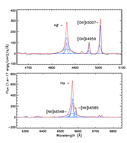
Figure 12: The Multi-Gaussian fit to the nearby region of H$\alpha$ and H$\beta$ line in the SDSS spectrum of PG 1244+026. The blue line shows Gaussian components separately, except for the narrow components and [NII]$\lambda$6585/6548 doublets which instead uses the same profile as the whole [OIII]$\lambda$5007 line. FeII lines have been subtracted (see Jin et al. 2012a)

7 Summary

In this paper, we presented a detailed spectral and timing analysis on a 123ks XMM-Newton observation of PG 1244+026, a NLS1 with very narrow Balmer lines and extreme mass accretion rate. The X-ray spectrum of PG 1244+026 contains a very steep hard X-ray power law and a strong/smooth soft X-ray excess. We show that the soft X-ray excess can be fit with an additional cool Comptonisation component or by extremely smeared, partially ionised reflection, but that both models require additional blackbody emission at the softest X-ray energies.

We then use a detailed timing analysis to distinguish between these two physical models for the soft X-ray excess. We derive the frequency-dependent fractional RMS and covariance spectra. For the fastest variability, the RMS spectrum has a clear soft excess, though this is smaller relative to the power law than in the time averaged spectrum. However, the spectrum of the variability correlated with the 4-10 keV lightcurve shows no soft excess over the same timescales. This clearly shows that the majority of the soft X-ray excess varies incoherently with the hard X-ray flux on fast timescales ($<5000$ s). A similar drop in coherence between hard and soft variability on the fastest timescales has previously also been seen in NGC4051 (M^cHardy et al. 2004). Here, combining the variability information with spectral models rules out a single reflection component making both the soft X-ray excess and the iron K line features as this predicts correlated flux variability in both hard and soft bands. However, it does not rule out more complex models, where there are multiple reflectors or some (small) contribution of ionised reflection to the soft bandpass as well as an additional soft X-ray component which emerges only below 1 keV.

By contrast, the spectrum of fast variability correlated with the 0.3-1 keV lightcurve has more soft X-ray excess than that of the HF RMS, as it includes all the soft excess variability seen in the HF RMS which is uncorrelated with the 4-10 keV emission. However, the drop in HF 0.3-1 keV covariance below 0.5 keV confirms the reality of the separate blackbody component required from the spectral fits.

Thus the fast variability data are clearly consistent with the spectral model in which the soft X-ray excess is a separate Comptonised component which provides the seed photons for the higher energy power law emission, but where the very softest energies are dominated by the disc itself. Conversely, it is inconsistent with a single reflection component producing the majority of the soft X-ray excess and the 4-10 keV emission.

The slower variability does not show a clear difference between the RMS and covariance spectra, showing that the source spectrum varies coherently on timescales longer than 10 ks. This could be interpreted in the spectral decomposition above in terms of propagation of fluctuations from the disc, through the soft X-ray excess region and into the high energy region (see e.g. Arévelo & Uttley 2006; Fabian et al. 2009).

We also assemble a broadband SED for PG 1244+026 from far infrared to hard X-ray, showing that this is dominated by the disc emission and that this extends into the soft X-ray bandpass, consistent with the spectral decomposition above. This system, and other NLS1 with similar spectral properties (e.g. RE J1034+396, RX J0136.9-3510), can then be used to constrain to the black hole spin via disc continuum fitting, as high black hole spin over-predicts the observed soft X-ray flux (D13).

References

- Arévalo & Uttley (2006) Arévalo P., Uttley P., 2006, MNRAS, 367, 801
- Arnaud (1996) Arnaud K. A., 1996, ASPC, 101, 17
- Ballantyne, Iwasawa & Fabian (2001) Ballantyne D. R., Iwasawa K., Fabian A. C., 2001, MNRAS, 323, 506
- Boroson & Green (1992) Boroson T. A., Green R. F., 1992, ApJS, 80, 109
- Boroson (2002) Boroson T. A., 2002, ApJ, 565, 78
- Crummy et al. (2006) Crummy J., Fabian A. C., Gallo L., Ross R. R., 2006, ApJ, 365, 1067
- Czerny et al. (2003) Czerny B., Nikołajuk M., Różańska A., Dumont A.-M., Loska Z., Zycki P. T., 2003, A&A, 412, 317
- Done & Nayakshin (2007) Done C., Nayakshin S., 2007, MNRAS, 377, L59
- Done et al. (2012) Done C., Davis S. W., Jin C., Blaes O., Ward, M., 2012, MNRAS, 420, 1848
- Done et al. (2013) Done C., Jin C., Middleton M., Ward M., 2013, MNRAS, accepted (arXiv:1306.4786) (D12)
- Edelson et al. (2002) Edelson R., Turner T. J., Pounds K., Vaughan S., Markowitz A., Marshall H., Dobbie P., Warwick R., 2002, ApJ, 568, 610
- Elvis et al. (1994) Elvis M., et al., 1994, ApJS, 95, 1
- Fabian et al. (2002) Fabian A. C., Ballantyne D.R., Merloni A., Vaughan S., Iwasawa K., Boller Th., 2002, MNRAS, 331, L35
- Fabian et al. (2004) Fabian A. C., Miniutti G., Gallo L., Boller Th., Tanaka Y., Vaughan S., Ross R. R., 2004, MNRAS, 353, 1071
- Fabian et al. (2009) Fabian A. C., et al., 2009, Nature, 459, 540
- Fiore et al. (1998) Fiore F., Matt G., Cappi M., Elvis M., Leighly K. M., Nicastro F., Piro L., Siemiginowska A., Wilkes B. J.,1998, MNRAS, 298, 103
- Gallo (2006) Gallo L. C., 2006, MNRAS, 368, 479
- Gierliński & Done (2004) Gierliński M., Done C., 2004, MNRAS, 349, L7
- Gierliński & Done (2006) Gierliński M., Done C., 2006, MNRAS, 371, L16
- Grupe (2004) Grupe D., 2004, AJ, 127, 1799
- Jin et al. (2009) Jin C., Done C., Ward M., Gierliński M., Mullaney J., 2009, MNRAS, 398, L16
- Jin, Ward & Done (2012b) Jin C., Ward M., Done C., 2012b, MNRAS, 422, 3268 (J12b)
- Jin, Ward & Done (2012c) Jin C., Ward M., Done C., 2012c, MNRAS, 425, 907 (J12c)
- Jin et al. (2012a) Jin C., Ward M., Done C., Gelbord J., 2012a, MNRAS, 420, 1825 (J12a)
- Kalberla et al. (2005) Kalberla P. M. W., Burton W. B., Hartmann D., Arnal E. M., Bajaja E., Morras R., Pöppel W. G. L., 2005, A&A, 440, 775
- Kolehmainen et al. (2011) Kolehmainen M., Done C., Díaz Trigo M., 2011, MNRAS, 416, 311
- Landt et al. (2011) Landt H., Elvis M., Ward M. J., Bentz M. C., Korista K. T., Karovska M., 2011, MNRAS, 414, 218
- Laor (1991) Laor A., 1991, ApJ, 376, 90
- Laor et al. (1997) Laor A., Fiore F., Elvis M., Wilkes B. J., McDowell J. C., 1997, ApJ, 477, 93
- Leighly (1999) Leighly K. M., 1999, ApJS, 125, 317
- Magdziarz et al. (1998) Magdziarz P., Blaes O. M., Zdziarski A. A., Johnson W. N., Smith D. A., 1998, MNRAS, 301, 179
- Markowitz et al. (2003) Markowitz A., Edelson R., Vaughan S., 2003, ApJ, 598, 935
- Marconi et al. (2008) Marconi A., Axon D. J., Maiolino R., Nagao T., Pastorini G., Pietrini P., Robinson A., Torricelli G., 2008, ApJ, 678, 693
- McHardy et al. (2004) McHardy I. M., Papadakis I. E., Uttley P., Page M. J., Mason K. O., 2004, MNRAS, 348, 783
- McHardy et al. (2007) McHardy I. M., Arévalo P., Uttley P., Papadakis I. E., Summons D. P., Brinkmann W., Page M. J., 2007, MNRAS, 382, 985
- Mehdipour et al. (2011) Mehdipour, M., Branduardi-Raymont, G., Kaastra, J. S., et al. 2011, A&A, 534, A39
- Middleton et al. (2011) Middleton M., Uttley P., Done C., 2011, MNRAS, 417, 250
- Middleton et al. (2009) Middleton M., Done C., Ward M., Gierliński M., Schurch N., 2009, MNRAS, 394,250
- Miller et al. (2007) Miller L., Turner T. J., Reeves J. N., George I. M., Kraemer S. B., Wingert B., 2007, A&A, 463, 131
- Nandra et al. (2007) Nandra K., O’Neill P. M., George I. M., Reeves, J. N., 2007, MNRAS, 382, 194
- Noda et al. (2011) Noda H., Makishima K., Yamada S., Torii S., Sakurai S., Nakazawa K., 2011, PASJ, 63, 925
- Noda et al. (2013) Noda H., Makishima K., Nakazawa K., Uchiyama H., Yamada S., Sakurai S., 2013, PASJ, 65, 4
- Osterbrock & Pogge (1985) Osterbrock D. E., Pogge R. W., 1985, ApJ, 297, 166
- Ponti et al. (2012) Ponti G., Papadakis I., Bianchi S., Guainazzi M., Matt G., Uttley P., Bonilla N. F., 2012, A&A, 542, A83
- Poutanen et al. (2008) Poutanen J., Zdziarski A. A., Ibragimov A., 2008, MNRAS, 389, 1427
- Reeves et al. (2008) Reeves J., Done C., Pounds K., Terashima Y., Hayashida K., Anabuki N., Uchino M., Turner M., 2008, MNRAS, 385, L108
- Revnivtsev & Gilfanov (2006) Revnivtsev M. G., Gilfanov, M. R., 2006, A&A, 453, 253
- Richards et al. (2006) Richards G. T. et al., 2006, ApJS, 166, 470
- Ross & Fabian (2005) Ross R. R., Fabian A. C., 2005, MNRAS, 358, 211
- Sim et al. (2010) Sim S. A., Proga D., Miller L., Long K. S., Turner T. J., 2010, MNRAS, 408, 1396
- Sobolewska & Życki (2006) Sobolewska M. A., Życki P. T., 2006, MNRAS, 370, 405
- Tatum et al. (2012) Tatum M. M., Turner T. J., Sim S. A., Miller L., Reeves J. N., Patrick A. R., Long K. S., 2012, ApJ, 752, 94
- Titarchuk (1994) Titarchuk L., 1994, ApJ, 434, 570
- Vaughan et al. (2003) Vaughan S., Edelson R., Warwick R. S., Uttley P., 2003, MNRAS, 345, 1271
- Veilleux et al. (2009) Veilleux et al., 2009, ApJS, 182, 628
- Vestergaard & Peterson (2006) Vestergaard M., Peterson B. M., 2006, ApJ, 641, 689
- Walton et al. (2013) Walton D. J., Nardini E., Fabian A. C., Gallo L. C., Reis R. C., 2013, MNRAS, 428, 2901
- Wilkinson & Uttley (2009) Wilkinson T., Uttley P., 2009, MNRAS, 397, 666
- Zdziarski et al. (1996) Zdziarski A. A., Johnson W. N., Magdziarz P., 1996, MNRAS, 283, 193