A Probabilistic Analysis of Kademlia Networks

Abstract

Kademlia [3] is currently the most widely used searching algorithm in p2p (peer-to-peer) networks. This work studies an essential question about Kademlia from a mathematical perspective: how long does it take to locate a node in the network? To answer it, we introduce a random graph ${\cal K}$ and study how many steps are needed to locate a given vertex in ${\cal K}$ using Kademlia’s algorithm, which we call the routing time. Two slightly different versions of ${\cal K}$ are studied. In the first one, vertices of ${\cal K}$ are labeled with fixed ids. In the second one, vertices are assumed to have randomly selected ids. In both cases, we show that the routing time is about $c\log n$, where $n$ is the number of nodes in the network and $c$ is an explicitly described constant.

1 Introduction to Kademlia

A p2p (peer-to-peer) network [4] is a computer network which allows sharing of resources like storage, bandwidth and computing power. Unlike traditional client-server architectures, in p2p networks, a participating computer (a node) is not only a consumer but also a supplier of resources. Nowadays, major p2p services in the internet often have millions of users. For an overview of p2p networks, see Steinmetz [5].

The huge size of p2p networks raises one challenge—among millions of nodes, how can a node find another one efficiently? To address this, a group of algorithms called dht (Distributed Hash Table) [6] was invented in the early 2000s, including Pastry [7], can [8], Chord [9], Tapestry [10], and Kademlia [3]. Created by Maymounkov and Mazières in 2002, Kademlia has become the de facto standard searching algorithm for p2p services. It is used by BitTorrent [11] and the Kad network [12], both of which have more than a million nodes.

Kademlia assigns each node an id chosen uniformly at random from $\{0,1\}^{d}$, the $d$-dimension hypercube, where $d$ is usually $128$ [12] or $160$ [11]. Thus we always refer to a node by its id. Given two ids $x=(x_{1},\ldots,x_{d})$ and $y=(y_{1},\ldots,y_{d})$, Kademlia defines their xor distance by

$$\delta(x,y)=\sum_{i=1}^{d}(x_{i}\oplus y_{i})\times 2^{d-i},$$

where $\oplus$ denotes the xor operation

$$u\oplus v=\begin{cases}1&\hbox{ if $u\neq v$,}\cr 0&\hbox{ otherwise.}\cr\end{cases}$$

Note that distance and closeness always mean xor distances between ids in this work.

Since it is almost impossible for a node to know where all other nodes are located, in Kademlia a node, say $x$, is only responsible for maintaining a table (a routing table) for a small number of other nodes ($x$’s neighbors). Roughly speaking, $\{0,1\}^{d}$ is partitioned into $d$ subsets, such that nodes in the same subset have similar distances to $x$. Within each subset, up to $k$ nodes’ information is recorded in a list (a $k$-bucket), where $k$ is a constant which usually equals $8$ [11], $10$ [12] or $20$ [13]. All of $x$’s $k$-buckets form $x$’s routing table.

When $x$ needs to locate node $y$ which is not in its routing table, $x$ sends queries to $\alpha$ of its neighbors which are closest to $y$, where $\alpha$ is a constant, sometimes chosen as $3$ [14] or $10$ [13]. A recipient of $x$’s message returns locations of $k$ of its own neighbors with shortest distance to $y$. With this information, $x$ again contacts $\alpha$ nodes that are closest to $y$. This approach (routing) repeats until no one closer to $y$ can be found. The efficiency of routing is critical for the overall performance of Kademlia. Its analysis is the topic of this work.

2 Our model

Consider a Kademlia network of $n$ nodes $X_{1},\ldots,X_{n}$. Writing ids as strings consisting of zeros and ones, from higher bits to lower bits, we can completely represent $X_{1},\ldots,X_{n}$ in a binary trie, as depicted in Fig. 1. A trie is an ordered tree data structure invented by Fredkin [15]. For more on tries, see Szpankowski [16]. Paths are associated with bit strings—$0$ corresponds to a left child, and $1$ to a right child. The bits encountered on a path of length $d$ to a leaf is the id, or value, of the leaf. In this manner, the binary trie, has height $d$, and precisely $n$ leaves of distance $d$ from the root.

Let $x=(x_{1},\ldots,x_{d})$ and $y=(y_{1},\ldots,y_{d})$ be two ids (leaves) in the trie. Let $\ell(x,y)$ be the length of the path from the root to $x$ and $y$’s lowest common ancestor, i.e., the length of $x$ and $y$’s common prefix. We have

$$\ell(x,y)=\max\{i:x_{1}=y_{1},\ldots,x_{i}=y_{i}\}\enspace.$$

It is easy to verify that $\ell(x,y)$ bounds the distance of $x$ and $y$ by

$$2^{d-\ell(x,y)-1}\leq\delta(x,y)<2^{d-\ell(x,y)}\enspace.$$

Thus if we partition $\{0,1\}^{d}\setminus\{x\}$ according to distances to $x$ as follows

$${{\cal D}}_{i}(x)=\{y:2^{i-1}\leq\delta(x,y)<2^{i}\},\quad i=1,\ldots,d,$$

then ${{\cal D}}_{i}(x)$ is equivalent to a subtree in the trie, in which each node shares a common prefix of length $i$ with $x$. Therefore, we have the equivalent definition

$${{\cal D}}_{i}(x)=\{y:\ell(x,y)=d-i\},\quad i=1,\ldots,d\enspace.$$

Let ${{\cal B}}_{i}(x)$ be the set of ids in the $k$-bucket of $x$ corresponding to ${{\cal D}}_{i}(x)$. In our model, we assume that if $|{{\cal D}}_{i}(x)|\leq k$, then ${{\cal B}}_{i}(x)={{\cal D}}_{i}(x)$. Otherwise, for all $A\subset{{\cal D}}_{i}(x)$ with $|A|=k$, we have

$${\tenmsbm P}\left\{{{\cal B}}_{i}(x)=A\right\}={{|{{\cal D}}_{i}(x)|}\choose k}^{-1}\enspace.$$

In other words, we fill up each $k$-bucket uniformly at random without replacement.

Figure 1: An example of Kademlia id trie and $k$-buckets. Given an id $x=(1,0,0)$, the trie is partitioned into subtrees ${\cal D}_{1}(x),{\cal D}_{2}(x),{\cal D}_{3}(x)$. Node $x$ maintains a $k$-bucket for each of these subtrees containing the information of up to $k$ nodes in the subtree, which we denote by ${\cal B}_{1}(x),{\cal B}_{2}(x),{\cal B}_{3}(x)$ respectively.

Consider a directed graph ${\cal K}$ with vertex set ${{\cal V}}=\{X_{1},\ldots,X_{n}\}$. Let its edge set be

$${\cal E}=\{(u,v):u,v\in{\cal V},\,v\in\cup_{i=1}^{d}{{\cal B}}_{i}(u)\}\enspace.$$

Put differently, we add a directed edge $(u,v)$ in ${\cal K}$ if and only if $v$ is in one of $u$’s $k$-buckets. When $\alpha=1$, only one node is queried at each step of routing, the search process starting at $x$ for $y$ can be seen as a path $\rho_{xy}$ in ${\cal K}$ (the routing path). It starts from vertex $x$, then jumps to the vertex that is closest to $y$ among all $x$’s neighbors. From there, it again jumps to the adjacent vertex that is closest to $y$. Let $y^{*}$ be the unique vertex with the shortest distance to $y$ in ${\cal K}$. Since the distance between the current vertex and $y^{*}$ decreases at each step until zero, $\rho_{xy}$ has no loop and always ends at $y^{*}$. In fact, ${\cal K}$ is always strongly connected.

Let $T_{xy}$ be the path length of $\rho_{xy}$. Since $T_{xy}$ equals the number of rounds of messages $x$ needs to send before routing ends, we call it the routing time. Our first main result assumes that $X_{1}=x_{1},\ldots,X_{n}=x_{n}$, where $x_{1},\ldots,x_{n}$ are all fixed $d$-bit vectors, which we call the deterministic id model. The randomness thus comes only from the filling of the $k$-buckets. We always assume that $d\geq\log_{2}n$, and we let $n\to\infty$ (and thus $d\to\infty$) in our asymptotic results. (Note that in this work $\log n$ denotes the natural logarithm of $n$.)

Theorem 2.1

In the deterministic id model, we have

$$\sup_{x_{1},\ldots,x_{n}}\sup_{x}\,\sup_{y}{\tenmsbm E}\left[T_{xy}\right]\leq({c_{k}}+o(1)){{\log n}},$$

$$\sup_{x_{1},\ldots,x_{n}}\sup_{x}{\tenmsbm E}\left[\sup_{y}T_{xy}\right]\leq({c_{k}^{\prime}}+o(1)){{\log n}},$$

$$\sup_{x_{1},\ldots,x_{n}}{\tenmsbm E}\left[\sup_{x}\,\sup_{y}T_{xy}\right]\leq({c_{k}^{*}}+o(1)){{\log n}},$$

where ${c_{k}},{c_{k}^{\prime}},{c_{k}^{*}}$ are constants depending only on $k$. In particular, we have ${c_{k}}=1/H_{k}$, where $H_{k}=\sum_{i=1}^{k}1/i$, also known as the $k$-th harmonic number.

The first inequality in this theorem gives an upper bound over the expected routing time between two fixed nodes. Since $c_{k}\leq c_{1}\leq 1/\log 2$, the first bound is better than the $\left\lceil\log_{2}n\right\rceil$ bound described by Maymounkov and Mazières in the original Kademlia paper [3]. The second inequality considers the expectation of the maximal routing time when the starting node is fixed, and a look-up is performed for each of the $n$ destinations. The third one considers the expectation of the maximal routing time in the whole network if all $n$ nodes were to look up all $n$ destinations.

Our second main result considers the situation when $X_{1},\ldots,X_{n}$ are selected uniformly at random from $\{0,1\}^{d}$ without replacement (the random id model). Given an id $x$, let $\widehat{x}$ denote the id that is farthest away from $x$ ($x$’s polar opposite). Since by symmetry ${T_{X_{1}{\widehat{X}_{1}}}},{T_{X_{2}{\widehat{X}_{2}}}},\ldots{T_{X_{n}{\widehat{X}_{n}}}}$ are identically distributed, we only need to study ${T_{X_{1}{\widehat{X}_{1}}}}$, which we denote by $\widehat{T}$.

Theorem 2.2 ([17])

In the random id model, we have

$${\widehat{T}\over{\log n}}\to{1\over g(k)}\qquad\hbox{in probability},$$

as $n\to\infty$, where $g(k)=H_{k}+O(1)$ is a function of $k$.

Since $\widehat{T}={T_{X_{1}{\widehat{X}_{1}}}}$, we see that

$${1\over g(k)}\leq{1\over{H_{k}}}\enspace.$$

However, we have almost identical behavior because $g(k)=H_{k}+O(1)$ as $k\to\infty$. Let $d=d(n)\geq\log_{2}n$. By the probabilistic method, Theorem 2.2 implies that for every $\epsilon>0$, there exists for every $n$ a non-repetitive sequence $(x_{1}(n),\ldots,x_{n}(n))\in(\{0,1\}^{d})^{n}$ of deterministic ids such that with probability going to one,

$${T_{X_{1}{\widehat{X}_{1}}}}\geq\left({1\over{g(k)}}-\epsilon\right)\log n\enspace.$$

In view of $g(k)=H_{k}+O(1)$, we thus see that the first bound of Theorem 2.1 is almost tight.

Recall that $y^{*}$ denotes the node that is closest to id $y$. If we look at the lowest common ancestor of $y^{*}$ and each hop of $\rho_{xy}$, then searching $y$ from $x$ can be seen as travelling downwards along the path from the root to the leaf $y^{*}$ in the trie, with the distance of each hop being random. In the random id model, when $n$ is large, we can approximate this process in a full binary trie with infinite depth. In Sect. 4, we sketch the proof of Theorem 2.2 which uses this method. This does not work in the deterministic id model as the structure of the id trie can be unbalanced. But in Sect. 3, we show that there is another way to bound the routing time.

Due to its success, Kademlia has aroused great interest among researchers. But this is the first time that it is studied from a mathematical perspective. Our results point out one important reason for the success of Kademlia — its routing algorithm, while being extremely simple, works surprisingly well. This work also shows that probabilistic methods together with the right choice of a data structure, a trie in our case, could significantly simplify the analysis of a problem which was previously considered too troublesome to analyze rigorously.

3 The deterministic ID model

In this section, we assume that $X_{1}=x_{1},\ldots,X_{n}=x_{n}$, where $x_{1},\ldots,x_{n}$ are fixed $d$-bits vectors. Note that the distribution of $T_{xy}$ is decided only by distances between vertices and the distance between $x$ and $y$. Thus, by rotating the hypercube, we can always assume $y$ to be a specific id, which we choose $\bar{1}=(1,1,\ldots,1)$.

Figure 2 depicts the first hop of $\rho_{x\bar{1}}$ as jumping from one leaf to another in the id trie. It is easy to see that if we always arrange branches representing $1$ to the right hand side, which we take as a convention, then the closer a leaf is to the right, the closer it is to $\bar{1}$. Thus the rightmost leaf in the trie, which we always denote by $y^{\prime}$, is closest to $\bar{1}$ and is thus the end point of $\rho_{x\bar{1}}$.

Write $\rho_{x\bar{1}}=(z_{0},z_{1},\ldots)$ where $z_{0}=x$. Let $i=d-\ell(z_{0},\bar{1})$. We can see from Fig. 2 that $z_{1}$, the first hop, must belong to ${\cal D}_{i}(z_{0})$, the highest subtree on the right hand side of $z_{0}$, which we denote by $S_{0}$. Since being $z_{0}$’s neighbor implies membership in one of $z_{0}$’s $k$-buckets, we have $z_{1}\in{\cal B}_{i}(z_{0})\subseteq S_{0}$. Recalling how ${\cal B}_{i}(z_{0})$ is decided, we can think of the first hop as selecting up to $k$ leaves from $S_{0}$ uniformly at random and choosing the rightmost one as $z_{1}$. Thus we can define of $\rho_{x\bar{1}}$ recursively as follows:

• Let $z_{0}=x$. Repeat the following step.

• Given $z_{t}$ and $t\geq 0$, let $S_{t}$ be highest subtree on the right hand side of $z_{t}$. If $S_{t}=\emptyset$, terminate. Otherwise select up to $k$ leaves from $S_{t}$ uniformly at random without replacement, and let the rightmost one be $z_{t+1}$.

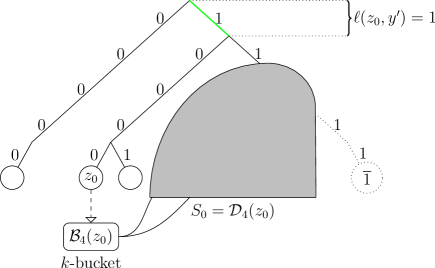
Figure 2: An example of the first hop of $\rho_{x\bar{1}}$ with $d=5$, $k=2$. Since $d-\ell(z_{0},y^{\prime})=4$, $z_{1}$ must be in subtree $S_{0}={\cal D}_{4}(z_{0})$, which is the highest subtree to the right of $z_{0}$. We choose up to $k$ leaves from $S_{0}$ uniformly at random without replacement, and let $z_{1}$ be the rightmost one.

Since $S_{0}\supset S_{1}\supset\dots\supset S_{T_{x\bar{1}}}=\emptyset$, by studying how quickly the sequence ${{(|S_{t}|)_{t\geq 0}}}$ decreases to $0$, we can bound how big $T_{x\bar{1}}$ could be. Although it is difficult to write the distribution of ${{(|S_{t}|)_{t\geq 0}}}$, we can approximate it with another sequence ${{(W_{t})_{t\geq 0}}}$. Let $B(k)$ be the minimum of $k$ independent uniform $[0,1]$ random variables. Let ${{(B_{t})_{t\geq 0}}}$ be a sequence of i.i.d. random variables with distribution $B(k)$. We define $W_{t}=|S_{0}|\times\prod_{s=1}^{t}B_{s}$.

Given two random variables $A$ and $B$, we say $A$ is stochastically smaller than $B$, denoted by $A\preceq B$, if and only if

$${\tenmsbm P}\left\{A\geq r\right\}\leq{\tenmsbm P}\left\{B\geq r\right\}\qquad\hbox{for all }r\in{\tenmsbm R},$$

where ${\tenmsbm R}$ is the set of real numbers. The random variable $W_{t}$ is stochastically larger than $|S_{t}|$, as there is a “trimming” effect at each hop. For example, the number of leaves between $z_{1}$ and $y^{\prime}$ has a distribution similar to $\lfloor W_{1}\rfloor$. But some of these leaves might not belong to $S_{1}$.

Figure 3: The “trimming” effect.

Lemma 1

For all $t\geq 1$, we have $|S_{t}|\preceq W_{t}$.

Lemma 2

For all $t\in{\tenmsbm N}$, we have:

$$\hbox{(i) }\qquad\sup_{x_{1},\ldots,x_{n}}\sup_{x}\sup_{y}{\tenmsbm P}\left\{T_{xy}\geq t\right\}\leq{\tenmsbm P}\left\{nB_{1}\ldots B_{t}\geq 1\right\},$$

$$\hbox{(ii) }\qquad\sup_{x_{1},\ldots,x_{n}}\sup_{x}{\tenmsbm P}\left\{\sup_{y}T_{xy}\geq t\right\}\leq n\times{\tenmsbm P}\left\{nB_{1}\ldots B_{t}\geq 1\right\},$$

$$\hbox{(iii)}\qquad\sup_{x_{1},\ldots,x_{n}}{\tenmsbm P}\left\{\sup_{x}\sup_{y}T_{xy}\geq t\right\}\leq n^{2}\times{\tenmsbm P}\left\{nB_{1}\ldots B_{t}\geq 1\right\}\enspace.$$

A beta random variable $B(a,b)$ has probability density function

$$f(x)={{\Gamma(a+b)}\over{\Gamma(a)\Gamma(b)}}\,x^{a-1}(1-x)^{b-1},\quad 0\leq x\leq 1,$$

where $\Gamma(z)$ is the gamma function $\Gamma(z)=\int_{0}^{\infty}e^{-t}t^{z-1}\,{\rm d}t.$ In order statistics theory, a basic result [18, chap.2.3] is that the $r$-th smallest of $m$ i.i.d. uniform random variables has beta distribution $B(r,m+1-r)$. Plugging in $r=1,m=k$, we have $B_{t}\,{\buildrel{\cal L}\over{=}}\,B(k)\,{\buildrel{\cal L}\over{=}}\,B(1,k)$ for all $t\in{\tenmsbm N}$. (For more about beta distribution, see [19, chap.25].) It is easy to check that for all $r>0$ and $t\in{\tenmsbm N}$, we have

$${\tenmsbm E}\left[\left(B_{1}\cdots B_{t}\right)^{r}\right]={\tenmsbm E}\left[B_{1}^{r}\right]^{t}={\tenmsbm E}\left[B(1,k)^{r}\right]^{t}=\left({{k!}\over{\prod_{i=1}^{k}(r+i)}}\right)^{t}\enspace.$$ (1)

By applying this moment bound, we have the following theorem:

Theorem 3.1

There exist constants ${c_{k}}$, ${c_{k}^{\prime}}$ and ${c_{k}^{*}}$ such that: (i) for all $c>{c_{k}}$,

$$\sup_{x_{1},\ldots,x_{n}}\sup_{x}\sup_{y}{\tenmsbm P}\left\{T_{xy}\geq c\log n\right\}\to 0\qquad\hbox{as }n\to\infty;$$

(ii) for all $c>{c_{k}^{\prime}}$,

$$\sup_{x_{1},\ldots,x_{n}}\sup_{x}{\tenmsbm P}\left\{\sup_{y}T_{xy}\geq c\log n\right\}\to 0\qquad\hbox{as }n\to\infty;$$

(iii) for all $c>{c_{k}^{*}}$,

$$\sup_{x_{1},\ldots,x_{n}}{\tenmsbm P}\left\{\sup_{x,y}T_{xy}\geq c\log n\right\}\to 0\qquad\hbox{as }n\to\infty\enspace.$$

In particular, we have ${c_{k}}=1/H_{k}$ where $H_{k}$ is the $k$-th harmonic number.

It is easy to check that $c_{1}^{\prime}=e$, since ${(r+1)/{\log(1+r)}}$ takes minimum value $e$ when $r=e-1$. But unlike ${c_{k}}$, we do not have closed forms for ${c_{k}^{\prime}}$ and ${c_{k}^{*}}$. Table 1 shows the numerical values of ${c_{k}},{c_{k}^{\prime}},{c_{k}^{*}}$ for $k=1,\ldots,10$.

Table 1: The numerical values of ${c_{k}},{c_{k}^{\prime}},{c_{k}^{*}}$ for $k=1,\ldots,10$.

$k$ ${c_{k}}$ ${c_{k}^{\prime}}$ ${c_{k}^{*}}$ 1 1 2.718281828 3.591121477 2 0.6666666667 1.673805050 2.170961287 3 0.5454545455 1.302556173 1.668389781 4 0.4800000000 1.105969343 1.403318015 5 0.4379562044 0.9817977138 1.236481558 6 0.4081632653 0.8950813294 1.120340102 7 0.3856749311 0.8304602569 1.034040176 8 0.3679369251 0.7800681679 0.9669189101 9 0.3534857624 0.7394331755 0.9129238915 10 0.3414171521 0.7058123636 0.8683482160

Lemma 3

We have

$$\lim_{k\to\infty}{c_{k}}\log k=\lim_{k\to\infty}{c_{k}^{\prime}}\log k=\lim_{k\to\infty}{c_{k}^{*}}\log k=1\enspace.$$

Remark 1

We are not providing precise inequalities with matching lower bounds. This can be done, but in that case, one could have to distinguish between many choices for $d$. We have already noted that $d\geq\log_{2}n$. We always have

$$T_{xy}\leq d\enspace.$$

Therefore, for $d$ very large, there is a danger of having routing times that are super-logarithmic in $n$. Our analysis shows that this is not the case. However, the precise behavior of $T_{xy}$, uniformly over all $x$,$y$ and $d$, requires additional analysis. The behavior for $d$ near $\log_{2}n$, $d=\Theta(\log n)$, and $d/\log n\to\infty$ is quite different.

Remark 2

The performance bounds of this section are of the form $c_{k}\log n$ with $c_{k}=1/H_{k}$. Although formulated for fixed $k$, they remain valid if $k$ is allowed to depend upon $n$. For example, if $k=\log n$—that is, the routing table size grows as $d\times\log n$—the expected routing time is bounded by

$$(1+o(1)){{\log n}\over{\log k}}\sim(1+o(1)){{\log n}\over{\log\log n}}\enspace.$$

Even more important is the possibility of having $O(1)$ routing time. With $k\sim n^{\theta}$ for $\theta\in(0,1)$, the routing table size for one computer grows as $d\times n^{\theta}$, and

$${\tenmsbm E}\left[\sup_{x}\sup_{y}T_{xy}\right]\leq{1\over\theta}+o(1)\enspace.$$

The parameter $\theta$ can be tweaked to obtain an acceptable compromise between storage and routing time.

4 The random ID model

In this section, we assume that $X_{1},\ldots,X_{n}$ are chosen uniformly at random from $\{0,1\}^{d}$ without replacement. Recall that $\widehat{X}_{1}$ denotes the id that is farthest from $X_{1}$. We sketch the proof that the distribution of $\widehat{T}\,{\buildrel{\rm def}\over{=}}\,{T_{X_{1}{\widehat{X}_{1}}}}$ has concentrated mass.

Since rotating the hypercube does not change the distribution of the routing time, we can always assume that $X_{1}=\bar{0}$ and $\widehat{X}_{1}=\bar{1}$, where $\bar{b}$ denotes the all-$b$ vector $(b,b,\ldots,b)$.

Write the routing path $\rho_{X_{1}\widehat{X}_{1}}=(z_{0},z_{1},\ldots)$. Let $a_{t}$ be the lowest common ancestor of $z_{t}$ and $y^{\prime}$, i.e., the rightmost leaf in the trie and the destination of routing. Then the sequence $(a_{0},a_{1},\ldots)$ can be seen as travelling downwards along the path from the root to $y^{\prime}$, i.e., the rightmost branch of the trie, with the distance of each hop being random.

This sequence can be defined equivalently as follows. Let $a_{0}$ be the root of the id trie. Let $z_{0}=\bar{0}$. From the right subtree of node $a_{t}$, select up to $k$ paths to the bottom uniformly at random without replacement. (This is equivalent to the choice of $k$ nodes to fill one $k$-bucket of $z_{t}$, the $t$-th hop in the search.) If that right subtree is empty, then the search terminates at $a_{t}$. Let $z_{t+1}$ be the leaf corresponding to the rightmost one of these selected paths. Let $a_{t+1}$ be the lowest common ancestor of $z_{t+1}$ and $y^{\prime}$. Let $L_{t+1}$ be the distance from $a_{0}$ to $a_{t+1}$. Let $R_{t+1}=L_{t+1}-L_{t}$, i.e., the distance of the $(t+1)$-th hop, which is also the distance between $a_{t}$ and $a_{t+1}$. Note that $\widehat{T}=t$ if and only if $\sum_{i=1}^{t}R_{i}=d$. Therefore, we can bound $\widehat{T}$ by studying the properties of ${(R_{t})_{t\geq 1}}$.

Now instead of the id trie of depth $d$, consider a full binary trie with infinite depth. Definite $(a_{0}^{\prime},a_{1}^{\prime},\ldots)$, the counterpart of $(a_{0},a_{1},\ldots)$ in this infinite trie, as follows. Let $a_{0}^{\prime}$ be the root of the infinite trie. From the right subtree of node $a_{t}^{\prime}$, select exactly $k$ infinite downwards paths uniformly at random. (Since the probability of selecting the same path more than once is zero, “without replacement” is not necessary anymore.) Let $z_{t+1}^{\prime}$ be the rightmost of these selected paths. Let $a_{t+1}^{\prime}$ be the lowest common node of $z_{t+1}^{\prime}$ and $\bar{1}$. Let $L_{t+1}^{\prime}$ be the distance from $a_{0}^{\prime}$ to $a_{t+1}^{\prime}$. Let $G_{t+1}=L_{t+1}^{\prime}-L_{t}^{\prime}$, i.e., the distance of $(t+1)$-th hop, which is also the distance between $a_{t}^{\prime}$ and $a_{t+1}^{\prime}$.

When $n$ is large (and thus $d$ is large), the behavior of ${(R_{t})_{t\geq 1}}$ and ${(G_{t})_{t\geq 1}}$ are very similar. But it is easy to see that, since each subtree of the infinite trie has exactly the same structure, ${(G_{t})_{t\geq 1}}$ is a sequence of i.i.d. random variables with distribution

$${\tenmsbm P}\left\{G_{1}\leq i\right\}=\left(1-{1\over{2^{i}}}\right)^{k}\qquad\hbox{for all }i\in{\tenmsbm N}.$$ (2)

In other words, ${(G_{t})_{t\geq 1}}$ is much easier to analyze. (Note that when $k=1$, $G_{1}$ is simply the geometric distribution.) And it is possible to couple the random variables $G_{t}$ and $R_{t}$.

When the downwards travel reaches the depth of $\log_{2}n$, the routing can not last much longer. In fact, in the id trie, a subtree whose root has depth at least $\log_{2}n$ has only $o(\log n)$ leaves with high probability [17]. Therefore, we define

$$T_{n}=\min\left\{t:t\geq 1,\sum_{i=1}^{t}G_{i}\geq\log_{2}n\right\}.$$

Lemma 4

We have

$${\tenmsbm E}\left[{T_{n}}\over{\log n}\right]\to{1\over{\log(2)\times{\tenmsbm E}\left[G_{1}\right]}},$$

as $n\to\infty$, and also

$${{T_{n}}\over{\log n}}\to{1\over{\log(2)\times{\tenmsbm E}\left[G_{1}\right]}}\qquad\hbox{in probability},$$

as $n\to\infty$.

Then, by coupling, we can show Lemma 5:

Lemma 5

We have

$${{\widehat{T}-T_{n}}\over{\log n}}\to 0\qquad\hbox{in probability},$$

as $n\to\infty$.

We omit the proof of these two lemmas due to space limitations. For details, see [17]. (For other proofs, see the appendix.)

Appendix

Proof of Lemma 1

Proof

Let $m,b$ be two positive integers. Let $Z(m,b)$ be the minimum of a sample of size up to $m$ selected uniformly at random from $\{0,1,\ldots,b-1\}$ without replacement. It is easy to check that

$$Z(m,b)\preceq b\times B(m)\qquad\hbox{for all }m,b\in{\tenmsbm N},$$

where ${\tenmsbm N}$ denotes the set of positive integers.

Consider step $t$ in the routing algorithm. Let $Z_{t}$ be the number of leaves to the right of $z_{t}$. Since up to $k$ leaves are selected uniformly at random without replacement from $S_{t-1}$ and the rightmost one is chosen as $z_{t}$, $Z_{t}$ has distribution $Z(k,|S_{t-1}|)$. Since $Z_{t}\geq|S_{t}|$, it follows that for all $r\in{\tenmsbm R}$ and $b\in{\tenmsbm N}$, we have

$${\tenmsbm P}\left\{|S_{t}|\geq r~{}|~{}|S_{t-1}|=b\right\} \leq{\tenmsbm P}\left\{Z_{t}\geq r~{}|~{}|S_{t-1}|=b\right\}$$

$$\leq{\tenmsbm P}\left\{b\times B(k)\geq r\right\}$$

$$={\tenmsbm P}\left\{b\times B_{t}\geq r\right\}\enspace.$$

Summing over all possible $b$, we have

$${\tenmsbm P}\left\{|S_{t}|\geq r\right\} =\sum_{b\in{\tenmsbm N}}{\tenmsbm P}\left\{|S_{t}|\geq r~{}|~{}|S_{t-1}|=b\right\}{\tenmsbm P}\left\{|S_{t-1}|=b\right\}$$

$$\leq\sum_{b\in{\tenmsbm N}}{\tenmsbm P}\left\{b\times B_{t}\geq r\right\}{\tenmsbm P}\left\{|S_{t-1}|=b\right\}$$

$$=\sum_{b\in{\tenmsbm N}}{\tenmsbm P}\left\{b\times B_{t}\geq r\cap|S_{t-1}|=b\right\}$$

$$={\tenmsbm P}\left\{B_{t}\times|S_{t-1}|\geq r\right\},$$

which implies $|S_{t}|\preceq B_{t}\times|S_{t-1}|$.

To finish the proof, we need a simple result from stochastic order theory [20, thm.1.A.3]. Given two nonnegative random variables $Y_{1}$ and $Y_{2}$ with $Y_{1}\preceq Y_{2}$, and a random variable $Z$ independent of both $Y_{1}$ and $Y_{2}$, we have

$$Y_{1}\times Z\preceq Y_{2}\times Z\enspace.$$

Recursively applying this inequality, we have

$$|S_{t}|\,\preceq\,B_{t}|S_{t-1}|\,\preceq\,B_{t}B_{t-1}|S_{t-2}|\,\preceq\,\dots\,\preceq\,\prod_{s=1}^{t}B_{s}|S_{0}|\,=\,W_{t}\enspace.\quad\squareforqed$$

Proof of Lemma 2

Proof

Note that $T_{xy}\geq t$ if and only if $|S_{t}|\geq 1$. It follows from the previous lemma that

$${\tenmsbm P}\left\{T_{xy}\geq t\right\}={\tenmsbm P}\left\{|S_{t}|\geq 1\right\}\leq{\tenmsbm P}\left\{|S_{0}|B_{1}\cdots B_{t}\geq 1\right\}\leq{\tenmsbm P}\left\{nB_{1}\cdots B_{t}\geq 1\right\}\enspace.$$

Clearly (ii) and (iii) follow from the union bound. ∎

Proof of Lemma 3

Proof

For $c_{k}$, this follows from ${c_{k}}=1/H_{k}$. For ${c_{k}^{\prime}}$ and ${c_{k}^{*}}$, note first

$${c_{k}}\leq{c_{k}^{\prime}}\leq{c_{k}^{*}}\enspace.$$

Next in the definition of ${c_{k}^{\prime}}$ and ${c_{k}^{*}}$, we obtain upper bounds by specifying a certain value of for $r$. So,

$${1\over{H_{K}}}\leq{c_{k}^{\prime}}\leq{c_{k}^{*}}\leq{{\sqrt{\log k}+2}\over\sum_{i=1}^{k}\log(1+\sqrt{\log k}/i)}=(1+o(1)){1\over{\log k}}.$$

The last equality follows easily by noticing that for all $\epsilon>0$, there exists $x_{0}>0$, such that

$$\log(1+x)\geq(1-\epsilon)x$$

for $0\leq x\leq x_{0}$. Thus, provided $k$ is so large that ${1\over{\sqrt{\log k}}}\leq x_{0}$, we have

$$\sum_{i=1}^{k}\log\left(1+{{\sqrt{\log k}}\over i}\right) \geq\sum_{i=\lceil\log k\rceil}^{k}\log\left(1+{{\sqrt{\log k}}\over i}\right)$$

$$\geq(1-\epsilon)\sum_{i=\lceil\log k\rceil}^{k}{{\sqrt{\log k}}\over i}$$

$$=(1-\epsilon)(H_{k}-H_{\lceil\log k\rceil})\sqrt{\log k}$$

$$\sim(1-\epsilon)(\log k)^{3/2}.$$

Therefore,

$${c_{k}^{*}}\leq{{\sqrt{\log k}+2}\over{(1-\epsilon)}(\log k)^{3/2}(1+o(1))}={{1+o(1)}\over{(1-\epsilon)\log k}}.$$

Since $\epsilon$ is arbitrary, we are done. ∎

Proof of Theorem 3.1

Proof

It follows from (i) of Lemma 2, the moment bound and equation (1) that for all and $r>0$ and $t\in N$, we have

$${\tenmsbm P}\left\{T_{xy}\geq t\right\}\leq{\tenmsbm P}\left\{nB_{1}\cdots B_{t}\geq 1\right\}\leq{\tenmsbm E}\left[B_{1}^{r}\right]n^{r}=\left({{k!}\over{\prod_{i=1}^{k}(r+i)}}\right)^{t}n^{r}\enspace.$$ (3)

Taking $t=c\log n$, we have

$$\log\left({\tenmsbm P}\left\{T_{xy}\geq c\log n\right\}\right)\leq\left(r-{{c}\times{\sum_{i=1}^{k}\log(1+r/i)}}\right)\log n\enspace.$$

Therefore, ${\tenmsbm P}\left\{T_{xy}\geq c\log n\right\}\to 0$ as $n\to\infty$ if

$$r-{{c}\times{\sum_{i=1}^{k}\log(1+r/i)}}<0\enspace.$$

Solving this inequality, we see that we need

$$c>h_{k}(r)\,{\buildrel{\rm def}\over{=}}\,{r\over{\sum_{i=1}^{k}\log(1+r/i)}}\enspace.$$

Thus, (i) follows if we take ${c_{k}}=\inf_{r>0}h_{k}(r)$. Simple calculations show that $h_{k}(r)$ increases on $(0,\infty)$. Therefore,

$${c_{k}}=\lim_{r\downarrow 0}h_{k}(r)=\lim_{r\downarrow 0}{1\over{\sum_{i=1}^{k}\log(1+r/i)^{1/r}}}={1\over{\sum_{i=1}^{k}1/i}}={1\over{H_{k}}}\enspace.$$

By a similar argument, (ii) and (iii) follows if we take

$${c_{k}^{\prime}}=\inf_{r>0}{{r+1}\over{\sum_{i=1}^{k}\log(1+r/i)}},\qquad{c_{k}^{*}}=\inf_{r>0}{{r+2}\over{\sum_{i=1}^{k}\log(1+r/i)}}\enspace.\quad\squareforqed$$

Proof of Theorem 2.1

Proof

For all $x\in{\cal V}$, $y\in\{0,1\}^{d}$ and $c>{c_{k}}$, we have

$${\tenmsbm E}\left[T_{xy}\right] =\sum_{t=1}^{\infty}{\tenmsbm P}\left\{T_{xy}\geq t\right\}$$

$$=\sum_{t=1}^{\lfloor c\log n\rfloor}{\tenmsbm P}\left\{T_{xy}\geq t\right\}+\sum_{t=\lceil c\log n\rceil}^{\infty}{\tenmsbm P}\left\{T_{xy}\geq t\right\}$$

$$\leq c\log n+\sum_{t=\lceil c\log n\rceil}^{\infty}\left({{k!}\over{\prod_{i=1}^{k}(r+i)}}\right)^{t}n^{r},\qquad\hbox{for all }(r>0).$$

The last inequality follows from the fact that probability is at most $1$ and equation (3). Note that the second term is a geometric series. We already showed that the first term in the series tends to $0$ as $n\to\infty$. The ratio between consecutive terms is $k!/\prod_{i=1}^{k}(r+i)<1$ for every fixed $r>0,k\geq 1$. Thus for all $\epsilon>0$, there exist $n_{0}\in{\tenmsbm N}$, such that for all $n>n_{0}$ we have

$${\tenmsbm E}\left[T_{xy}\right]\leq({c_{k}}+\epsilon)\log n,$$

or simply

$${\tenmsbm E}\left[T_{xy}\right]\leq({c_{k}}+o(1))\log n\enspace.$$

(ii) and (iii) follow by similar arguments. ∎

Proof of Theorem 2.2

Proof

It follows from (2) that

$${\tenmsbm E}\left[G_{1}\right]\geq\int_{0}^{\infty}1-\left(1-{1\over{2^{x}}}\right)^{k}{\rm d}x={{H_{k}}\over{\log 2}},$$

and

$${\tenmsbm E}\left[G_{1}\right]\leq 1+\int_{0}^{\infty}1-\left(1-{1\over{2^{x}}}\right)^{k}{\rm d}x=1+{{H_{k}}\over{\log 2}}\enspace.$$

Therefore,

$$g(k)\,{\buildrel{\rm def}\over{=}}\,\log(2)\times{\tenmsbm E}\left[G_{1}\right]=H_{k}+O(1)\enspace.$$

It follows from Lemma 4 that Lemma 5 that

$${{\widehat{T}}\over{\log n}}\to{1\over g(k)}\qquad\hbox{in probablity},$$

as $n\to\infty$. ∎

References

- [1] Davis, C., Fernandez, J., Neville, S., McHugh, J.: Sybil attacks as a mitigation strategy against the storm botnet. In: Proceedings of the 3rd International Conference on Malicious and Unwanted Software, Malware ’08. (2008) 32 – 40
- [2] Davis, C., Neville, S., Fernandez, J., Robert, J.M., McHugh, J.: Structured peer-to-peer overlay networks: Ideal botnets command and control infrastructures? In: Computer Security - ESORICS 2008. Volume 5283 of LNCS. Springer, Berlin/Heidelberg, Germany (2008) 461–480
- [3] Maymounkov, P., Mazières, D.: Kademlia: A peer-to-peer information system based on the xor metric. In: Peer-to-Peer Systems. Volume 2429 of LNCS. Springer, Berlin/Heidelberg, Germany (2002) 53 – 65
- [4] Schollmeier, R.: A definition of peer-to-peer networking for the classification of peer-to-peer architectures and applications. In: Proceedings of 1st International Conference on Peer-to-Peer Computing. (2001) 101 – 102
- [5] Steinmetz, R., Wehrle, K.: Peer-to-Peer Systems And Applications. LNCS. Springer, Berlin/Heidelberg, Germany (2005)
- [6] Balakrishnan, H., Kaashoek, M.F., Karger, D., Morris, R., Stoica, I.: Looking up data in P2P systems. Communications of the ACM 46(2) (2003) 43 – 48
- [7] Rowstron, A., Druschel, P.: Pastry: Scalable, decentralized object location, and routing for large-scale peer-to-peer systems. In: Middleware 2001. Volume 2218 of LNCS. Springer, Berlin/Heidelberg, Germany (2001) 329 – 350
- [8] Ratnasamy, S., Francis, P., Handley, M., Karp, R., Shenker, S.: A scalable content-addressable network. SIGCOMM Computer Communication Review 31(4) (2001) 161 – 172
- [9] Stoica, I., Morris, R., Karger, D., Kaashoek, M.F., Balakrishnan, H.: Chord: A scalable peer-to-peer lookup service for internet applications. SIGCOMM Computer Communication Review 31(4) (August 2001) 149–160
- [10] Zhao, B.Y., Huang, L., Stribling, J., Rhea, S.C., Joseph, A.D., Kubiatowicz, J.D.: Tapestry: A resilient global-scale overlay for service deployment. IEEE Journal on Selected Areas in Communications 22 (2004) 41 – 53
- [11] Crosby, S.A., Wallach, D.S.: An analysis of BitTorrent’s two Kademlia-based dhts. Rice University, Houston, TX, USA (2007)
- [12] Steiner, M., En-Najjary, T., Biersack, E.W.: A global view of Kad. In: Proceedings of the 7th ACM SIGCOMM Conference on Internet Measurement. IMC ’07, New York, NY, USA, ACM (2007) 117 – 122
- [13] Falkner, J., Piatek, M., John, J.P., Krishnamurthy, A., Anderson, T.: Profiling a million user dht. In: Proceedings of the 7th ACM SIGCOMM conference on Internet measurement. IMC ’07, New York, NY, USA, ACM (2007) 129 – 134
- [14] Steiner, M., En-Najjary, T., Biersack, E.W.: Exploiting Kad: possible uses and misuses. SIGCOMM Computer Communication Review 37(5) (2007) 65 – 70
- [15] Fredkin, E.: Trie memory. Communications of the ACM 3(9) (1960) 490 – 499
- [16] Szpankowski, W.: Average Case Analysis of Algorithms on Sequences. Wiley, Hoboken, NJ, USA (2011)
- [17] Cai, X.S.: A probabilistic analysis of kademlia networks. Master’s thesis, McGill University (August 2012)
- [18] David, H., Nagaraja, H.: Order Statistics. Wiley, Hoboken, NJ, USA (2003)
- [19] Johnson, N., Kotz, S., Balakrishnan, N.: Continuous Univariate Distributions. Volume 2. Wiley, Hoboken, NJ, USA (1995)
- [20] Shaked, M., Shanthikumar, J.: Stochastic Orders. Springer Series in Statistics. Springer, New York, NY, USA (2007)