Competitive Adsorption of a Two-Component Gas on a Deformable Adsorbent

Abstract

We investigate the competitive adsorption of a two-component gas on the surface of an adsorbent whose adsorption properties vary in adsorption due to the adsorbent deformation. The essential difference of adsorption isotherms for a deformable adsorbent both from the classical Langmuir adsorption isotherms of a two-component gas and from the adsorption isotherms of a one-component gas taking into account variations in adsorption properties of the adsorbent in adsorption is obtained. We establish bistability and tristability of the system caused by variations in adsorption properties of the adsorbent in competitive adsorption of gas particles on it. Conditions under which adsorption isotherms of a binary gas mixture have two stable asymptotes are derived. It is shown that the specific features of the behavior of the system under study can be described in terms of a potential of the known explicit form.

PACS numbers: 68.43.-h; 68.43.Mn; 68.43.Nr; 68.35.Rh

1 Introduction

Problems of adsorption on the surface of different bodies belong to a wide class of problems of physics, chemistry, and biology that are very important both from the theoretical point of view and for various practical applications. The results of numerous investigations show that adsorption of particles leads to considerable changes in physical and chemical characteristics of adsorbents. Detailed analysis of the changes in the properties of the adsorbent surface due to adsorption is given, e.g., in [1, 2, 3, 4, 5, 6, 7, 8, 9, 10, 11].

Since processes of adsorption and desorption are obligatory stages of heterogeneous-catalytic reactions, the results of the adsorption theory are extremely important for investigation of various problems of heterogeneous catalysis [12, 13, 14, 15, 16, 17].

Generalizations of the classical Langmuir adsorption theory aimed at a more correct description of the adsorbent surface and adsorbed particles give the qualitatively new behavior of the amount of adsorbed substance and its kinetics. An extensive material obtained on the basis of different models and applications to various problems of adsorption and catalysis are widely presented in the literature (see, e.g., [8, 13, 14, 15, 16, 17, 18, 19, 20, 21, 22]). In particular, due to lateral interactions between adparticles, adsorption isotherms can have a hysteresis shape, and different structural changes in the adsorbent surface occur (reviews of the theoretical and experimental results are given, e.g., in [8, 9, 10, 11, 19, 20, 21, 22]). In turn, a qualitative change in the surface structure in adsorption leads to a series of specific features of oscillatory surface reactions and formation of different spatiotemporal patterns (for the oscillatory kinetics in heterogeneous catalysis and related problems, see, e.g., the reviews [23, 24, 25] and the monograph [26]).

It is established in [27] that, parallel with lateral interactions between adparticles, there is another factor (the adsorption-induced deformation of an adsorbent) leading to hysteresis-shaped isotherms of localized adsorption of a one-component gas on the flat energetically homogeneous surface of a solid adsorbent. It is worth noting that, as early as in 1938, in [28], Zeldovich based on the idea of a change in adsorption properties of the adsorbent surface in adsorption, predicted a hysteresis of adsorption isotherms if the typical time of adsorption and desorption is much less than the relaxation time of the surface.

In recent years, it has been established an essential influence of memory effects on the surface diffusion of adparticles over the adsorbent surface in the case where the relaxation time of the adsorbent is comparable (or greater than) with typical times for moving adparticles (see, e.g., the review [29] and references therein). Dynamical changes in properties of the surface by moving particles are taken into account in some models (e.g., in [30, 31]), which, to some extent, is similar to the Zeldovich idea of an absorbent varying its adsorption properties in adsorption.

Since an actual adsorbate includes several species of particles, in adsorption, particles of different species compete for adsorption sites. This leads not only to a decrease in the number of adparticles of a species relative to that for one-component adsorption [19, 21, 22, 32, 33] but also to the qualitative change in the shape of adsorption isotherms with regard for lateral interactions between adparticles [20]. In view of hysteresis-shaped isotherms of localized adsorption of a one-component gas on the flat surface of a solid adsorbent due to the adsorption-induced deformation of an adsorbent [27], it is of interest to investigate the influence of this factor on changes in the classical extended Langmuir adsorption isotherms of a multicomponent gaseous system.

In the present paper, we study specific features of adsorption isotherms of a two-component gas on the surface of a solid adsorbent whose adsorption properties vary in adsorption.

A model of adsorption of a two-component gas taking into account variations in adsorption properties of an adsorbent caused by its deformation in adsorption is proposed in Sec. 2. We obtain a system of equations that describes the kinetics of the surface coverage and the displacement of adsorption sites. For each species of adparticles, it is introduced the dimensionless coupling parameter equal to the normalized maximum increment of the activation energy for desorption due to the adsorbent deformation in one-component adsorption. The influence of the adsorbent deformation on the adsorption isotherms of adparticles of both species is investigated in Sec. 3. It is established a considerable redistribution of the amount of adsorbed substances as compared with that in the classical case even for a negligible quantity of particles of one species in a gas mixture. The obtained adsorption isotherms essentially depend on the coupling parameters and differ both from the Langmuir adsorption isotherms of a two-component gas and from the adsorption isotherms of a one-component gas for an adsorbent whose adsorption properties vary in adsorption. We establish bistability and tristability of the system caused by variations in adsorption properties of the adsorbent in competitive adsorption. Conditions under which adsorption isotherms of a binary gas mixture have two stable asymptotes are derived. In Sec. 4, within the framework of the overdamped approximation and essential difference in the linear relaxation times of the dynamical variables, the behavior of the system under study is described in terms of a potential whose explicit form is obtained. The specific features of isotherms of competitive adsorption are explained with the use of the (single-, two-, or three-well) potential.

2 General Relations

We consider localized monolayer competitive adsorption of particles of a two-component gas on the flat surface of a solid adsorbent using the classical Langmuir model generalized to the case of variations in adsorption properties of the adsorbent in adsorption–desorption of gas particles [27]. Gas particles are adsorbed on adsorption sites located at the adsorbent surface and total number of sites $N$ does not change in time. All adsorption sites have equal adsorption activity (energetically homogeneous surface) and each adsorption site can be bound only with one gas particle. We introduce the Cartesian coordinate system with the origin on the adsorbent surface and the $0X$-axis directed into the adsorbent so that the adsorbent and the gas occupy the regions $x\geq 0$ and $x<0$, respectively.

Following [27], we simulate each vacant adsorption site by a one-dimensional linear oscillator of mass $m_{0}$ that oscillates perpendicularly to the surface about its equilibrium position $x=0$.

The binding of a gas particle with an adsorption site is accompanied by a change in the spatial distribution of the charge density of the bound adsorption site as compared with that of a vacant one. This change depends on the nature of adsorption bonds and specific features of both the adsorbent and gas particles (see, e.g., [3, 8, 9, 23, 24, 25, 26, 34]).

This leads to a change in the interaction of the bound adsorption site with neighboring atoms of the adsorbent located both on the surface and in the nearest subsurface region. As a result, the resulting force acting on the bound adsorption site changes as against that acting on the vacant adsorption site. This can be regarded as the appearance of a certain adsorption-induced force $\vec{F}_{n}(\vec{r},t)$ acting on the adsorption site occupied by an adparticle of species $n=1,2$ (here and below, the subscript $n=1,2$ denotes the species of particles), where $\vec{r}$ is the running coordinate of the adsorption site. Under the action of this force, the bound adsorption site tends to a new equilibrium position. However, as soon as the adparticle leaves the adsorption site, the last becomes vacant and relaxes to its nonperturbed equilibrium position $x=0$. For the subsequent adsorption of other gas particle on this vacant adsorption site, two essentially different situations are possible: a gas particle occupies the site after or before it reaches the nonperturbed equilibrium position. In the first case, a new adparticle on the adsorption site does not “fill” its earlier occupation by previous adparticles. In the second, a particle is adsorbed on the surface locally deformed by the previous adparticle (not necessarily of the same species), i.e., the retardation of relaxation of the surface occurs or, in other words, adsorption with memory takes place.

We consider the case where the force $\vec{F}_{n}(\vec{r},t)$ is normal to the boundary and depends only on the coordinate $x$:   $\vec{F}_{n}(\vec{r},t)=\vec{e}_{x}\,F_{n}(x,t)$, where $\vec{e}_{x}$ is the unit vector along the $0X$-axis.

The force $\vec{F}_{n}(\vec{r},t)$ acts on the adsorption site only during discrete time intervals where the site is bound. Thus, at any instant, the adsorption site is in one of the three states: vacant or bound with adparticle of species 1 or 2. Instead, we consider the approximation of a time-continuous adsorption-induced force $\vec{F}(\vec{r},t)$, which corresponds to an adsorption site permanently bound with an adparticle with the time-dependent probability (the mean occupancy of adparticle on an adsorption site) equal to the surface coverage by adparticles of species $n$, $\theta_{n}=N_{n}(t)/N$, where $N_{n}(t)$ is the number of adsorption sites occupied by adparticles of species $n$ at the time $t$. Since an adsorption site can be bound only with one adparticle, $\vec{F}(\vec{r},t)=\vec{F}_{1}(x)\,\theta_{1}+\vec{F}_{2}(x)\,\theta_{2}$, where $\vec{F}_{n}(x)=\vec{e}_{x}\,F_{n}(x)$, and, hence, $\vec{F}(\vec{r},t)=\vec{e}_{x}\,F(x,t),\ F(x,t)=F_{1}(x)\,\theta_{1}+F_{2}(x)\,\theta_{2}$. This approximation is similar to the mean-field approximation used in the adsorption theory taking into account lateral interactions between adparticles (see, e.g., [8, 21]). Expanding $F_{n}(x)$ in the Taylor series in the neighborhood of $x=0$ and keeping only the first term of the expansion, and expressing the adsorption-induced force $\vec{F}_{n}(x)$ in terms of the potential, $F_{n}(x)=-\frac{dV_{n}(x)}{dx}$, we get

$$V_{n}(x)\approx-\chi_{n}\,x\,,\qquad n=1,2,$$ (1)

where

$$\left.\chi_{n}=-\frac{dV_{n}(x)}{dx}\right|_{x=0}$$

is the constant adsorption-induced force acting on the adsorption site occupied by an adparticle of species $n$.

We introduce the dimensionless quantity $G=\chi_{2}/\chi_{1}$, which is positive or negative for parallel ($\mathop{\rm sign}\nolimits\,\chi_{1}=\mathop{\rm sign}\nolimits\,\chi_{2}$) or antiparallel ($\mathop{\rm sign}\nolimits\,\chi_{1}=-\mathop{\rm sign}\nolimits\,\chi_{2}$) adsorption-induced forces, respectively.

Disregarding the internal motions in the adparticle–adsorption site system, i.e., considering the motion of the bound adsorption site as a whole, and taking into account a change in the mass of the oscillator in adsorption within the framework of this approximation, we obtain the following equation of motion of an oscillator of variable mass in the adsorption-induced force field:

$$\frac{d}{dt}\biggl{(}m_{eff}(\Theta)\frac{dx}{dt}\biggr{)}+\alpha\frac{dx}{dt}+\varkappa\,x=\chi_{1}\,\theta_{1}+\chi_{2}\,\theta_{2}\,,$$ (2)

where $\varkappa$ is the restoring force constant, $\alpha$ is the friction coefficient, $m_{eff}(\Theta)=m_{0}+m_{1}\,\theta_{1}+m_{2}\,\theta_{2}$ is the effective mass of the oscillator that varies in adsorption, $m_{n}$ is the mass of an adparticle of species $n$, and the symbol $\Theta\equiv\{\theta_{1},\,\theta_{2}\}$ denotes a collection of the surface coverages. Since $\theta_{n}\leq 1$, the effective mass of the oscillator is lesser than $M=m_{0}+m_{1}+m_{2}$.

It follows from Eq. (2) that, due to adsorption, the equilibrium position of the oscillator $x=0$ shifts to the new one $x^{eq}(\Theta)$ defined by the relation

$$x^{eq}(\Theta)=x_{1}^{eq}(\theta_{1})+x_{2}^{eq}(\theta_{2})\,,$$ (3)

where $x_{n}^{eq}(\theta_{n})=x_{n}^{max}\,\theta_{n}$ is the equation for determination of the equilibrium position of the oscillator in adsorption of a one-component gas of species $n$ and $x_{n}^{max}\equiv x_{n}^{eq}(1)=\chi_{n}/\varkappa$ is the maximum stationary displacement of the oscillator from its nonperturbed equilibrium position $x=0$ in the case of the total surface coverage ($\theta_{n}=1$).

Within the framework of the used approximation, the forces of lateral interactions between adparticles are parallel to the adsorbent surface and the adsorption-induced forces $\vec{F}_{n}(x)$ are perpendicular to the surface, which means that the forces $\vec{F}_{n}(x)$ are caused by the interaction of bound adsorption sites with the nearest subsurface atoms of the adsorbent. Nevertheless, the lateral interactions between adparticles affect the adsorption-induced force $\vec{F}(\vec{r},t)$ (and, hence, a normal displacement of the plane of adsorption sites) via the surface coverages $\theta_{1}$ and $\theta_{2}$.

In the Langmuir theory of kinetics on a nondeformable adsorbent ($\chi_{n}=0,\ n=1,2$) neglecting interactions between adparticles, the rate constants for adsorption and desorption $k_{n}^{a}$ and $k_{n}^{d}$ of particles of species $n$, respectively, do not depend on the concentration of particles in the gas phase and are defined by the Arrhenius relations

$$k_{n}^{a}=k_{n}^{+}\exp{\biggl{(}-\frac{E_{n}^{a}}{k_{B}T}\biggr{)}}\,,\qquad k_{n}^{d}=k_{n}^{-}\exp{\biggl{(}-\frac{E_{n}^{d}}{k_{B}T}\biggr{)}}\,,\qquad n=1,2,$$ (4)

where $E_{n}^{a}$ and $E_{n}^{d}$ are the activation energies for adsorption and desorption, respectively, $k_{n}^{+}$ and $k_{n}^{-}$ are the pre-exponential factors, $T$ is the absolute temperature, and $k_{B}$ is the Boltzmann constant.

The Hamiltonian of the adparticles–adsorbent system contains the term $-\chi_{1}\,x\,N_{1}-\chi_{2}\,x\,N_{2}$ caused by the adsorbent deformation in adsorption due to the adsorption-induced force field $F(x,t)$. This implies that an adparticle of species $n$ is not only in a potential well of constant depth $E_{n}^{d}$ but also in the adsorption-induced potential $V_{n}(x)$. For parallel adsorption-induced forces, an adparticle of any species is in a deeper potential well than on a nondeformable adsorbent. As a result, in the case at hand, for desorption of an adparticle of species $n$, it must get an energy greater than $E_{n}^{d}$ by the value $|V_{n}(x)|=\chi_{n}\,x$, which can be regarded as the increment of the activation energy for desorption $E_{n}^{d}$ of an adparticle of species $n$ caused by the adsorbent deformation. For antiparallel adsorption-induced forces, the increments $\chi_{n}\,x$ of the activation energies for desorption $E_{n}^{d}$ of adparticles of different species $n$ have opposite signs. Thus, the adsorbent deformation increases the activation energy for desorption of adparticles of one species and decreases the activation energy for desorption of adparticles of another species. Note that the quantities $E_{n}^{d}$ and $\chi_{n}\,x$ can be interpreted as the first and second terms, respectively, of the Taylor series of the coordinate-dependent activation energy for desorption $E_{n}^{d}(x)$.

It is well known that lateral interactions between adparticles essentially change adsorption isotherms of a binary gas mixture (see, e.g., [20]). In the present paper, to illustrate that there is another factor (the adsorption-induced deformation of the adsorbent) leading to qualitative changes in isotherms of competitive adsorption of a two-component gas, we do not take into account lateral interactions between adparticles.

The adsorbent deformation in adsorption affects the desorption rates of adparticles and, hence, the surface coverage. Assuming that the pre-exponential factors $k_{n}^{-}$ are not changed, we obtain the following expression for the rate coefficients for desorption:

$$k_{n}^{d}(x)=k_{n}^{d}\exp{\biggl{(}-\frac{\chi_{n}\,x}{k_{B}T}\biggr{)}}.$$ (5)

Thus, the rate coefficients for desorption (5) are coordinate-dependent functions, and gas particles are adsorbed on the surface whose adsorption characteristics vary with time.

According to (5), for $G>0$, the desorption rates of adparticles of both species decrease due to the adsorbent deformation in adsorption. For $G<0$, the joint action of adparticles of both species on the adsorbent leads to the opposite results: the desorption rate of adparticles decreases for one species and increases for another.

With regard for variations in adsorption properties of the adsorbent in adsorption, the kinetics of the surface coverages is described by the equations

$$\frac{d\theta_{n}}{dt}=k_{n}^{a}C_{n}\,\theta_{0}-k_{n}^{d}\,\theta_{n}\,\exp{\biggl{(}-\frac{\chi_{n}\,x}{k_{B}T}\biggr{)}},\qquad n=1,2,$$ (6)

where $C_{n}$ is the concentration of particles of species $n$ in the gas phase that is kept constant, $\theta_{0}=1-\theta_{+}=N_{0}(t)/N$ is the vacant part of the surface, $\theta_{+}=\theta_{1}+\theta_{2}=N_{b}(t)/N$ is the surface coverage by adparticles of both species, $N_{b}(t)=N_{1}(t)+N_{2}(t)$ and $N_{0}(t)$ are, respectively, the numbers of occupied and vacant adsorption sites at the time $t$, $N_{b}(t)+N_{0}(t)=N$.

Setting in (6) $\chi_{n}=0$, we obtain the known system of two linear equations that describes the Langmuir kinetics of adsorption of a two-component gas [18].

Introducing the dimensionless coordinate of oscillator $\xi=x/x_{1}^{max}$, we obtain the following autonomous system of three nonlinear differential equations that describes the kinetics of the surface coverages and the normal displacement of adsorption sites in localized adsorption with regard for variations in adsorption properties of the adsorbent in adsorption:

$$\left\{\begin{array}[]{l}\dfrac{d\theta_{n}}{dt}=k_{n}^{a}C_{n}\,\theta_{0}-k_{n}^{d}\,\theta_{n}\exp{\left(-\dfrac{g_{n}}{G_{n}}\,\xi\,\right)},\qquad\quad n=1,2,\vspace{-2mm}\\ \\ \dfrac{d}{dt}\biggl{(}m_{eff}(\Theta)\dfrac{d\xi}{dt}\biggr{)}+\alpha\dfrac{d\xi}{dt}=\varkappa\,\bigl{(}\theta_{1}+G\,\theta_{2}-\xi\bigr{)}.\end{array}\right.$$ (10)

Here, the dimensionless quantity

$$g_{n}=|V_{n}|/k_{B}T,\qquad n=1,2,$$ (11)

called a coupling parameter, is the maximum increment of the activation energy for desorption (normalized by $k_{B}\,T$) due to the adsorbent deformation in adsorption of a one-component gas of species $n$, $\ V_{n}\equiv V_{n}(x_{n}^{max})=-\chi_{n}^{2}/\varkappa$, $\,G_{1}=1$, $\,G_{2}\equiv G$, $\,g_{2}=g_{1}\,G^{2}$.

Setting in (7) $C_{2}=0$ and $\theta_{2}=0$, we obtain the system of two differential equations that describes the kinetics of the amount of a one-component gas of species 1 adsorbed on a deformable adsorbent [27].

The average coordinate-dependent residence times of adparticles on the surface of a deformable adsorbent $\tau_{n}^{d}(\xi)=1/k_{n}^{d}(\xi)\,,\ n=1,2$,

$$\tau_{1}^{d}(\xi)=\tau_{1}^{d}\exp{\left(g_{1}\,\xi\,\right)},\qquad\qquad\tau_{2}^{d}(\xi)=\tau_{2}^{d}\exp{\left(g_{1}\,G\,\xi\,\right)},$$ (12)

increase for $G>0$ as against the classical residence times

$$\tau_{n}^{d}=\frac{1}{k_{n}^{d}}\,,\qquad\qquad n=1,2,$$ (13)

and, furthermore, the greater the displacement of adsorption sites from their nonperturbed equilibrium position, the more this increase. Since the residence time of adparticles with a greater value of $|\chi_{n}|$ increases greater, the surface is more intensively occupied by particles of this species and this process rapidly grows with $\xi$. Denoting the ratio of the residence times of adparticles of different species on the adsorbent surface by

$$R(\xi)=\frac{\tau_{2}^{d}(\xi)}{\tau_{1}^{d}(\xi)}\,,$$ (14)

we obtain

$$R(\xi)=R_{0}\,w(\xi),$$ (15)

where

$$R_{0}\equiv R(0)=\frac{\tau_{2}^{d}}{\tau_{1}^{d}}$$ (16)

is the ratio of the residence times of adparticles of different species on the nondeformable adsorbent and the quantity

$$w(\xi)=\exp{\Bigl{(}g_{1}\left(G-1\right)\xi\Bigr{)}}$$ (17)

characterizes a variation in ratio (13) due to the different action of adparticles of both species on the adsorbent. In the special case of the identical action of all adparticles on the adsorbent ($\chi_{1}=\chi_{2}$), we have $w(\xi)=1$. According to (14), for $G>1$, the quantity $w(\xi)$ can reach large values, which essentially affects the surface coverages $\theta_{1}$ and $\theta_{2}$.

Expressions (9), (11), (12), and (14) are also true for $G<0$. However, in this case, the adsorbent deformation caused by the joint action of adparticles of both species leads to an increase in the residence time of adparticles of one species and a decrease in the residence time of adparticles of other species as against the classical residence times (10).

3 Stationary Case

3.1 General Relations

In the stationary case, system (7) is reduced to the system

$$\left\{\begin{array}[]{llll}\ell_{1}&=&\dfrac{\theta_{1}}{\theta_{0}}\,\exp{\left(-g_{1}\,\xi\right)}\,,\vspace{2mm}\\ \ell_{2}&=&\dfrac{\theta_{2}}{\theta_{0}}\,\exp{\left(-g_{1}\,G\,\xi\right)}\,,\vspace{2mm}\\ \xi&=&\theta_{1}+G\,\theta_{2}\,,\end{array}\right.$$ (21)

where $\ell_{n}=C_{n}\,K_{n}$ is the dimensionless concentration of gas particles of species $n=1,2$ and $K_{n}=k_{n}^{a}/k_{n}^{d}$ is the adsorption equilibrium constant for a one-component gas of species $n$ in the linear case ($\chi_{n}=0$).

After simple transformations, we obtain the following expressions for the surface coverages:

$$\theta_{1} = \frac{\xi}{1+G\,S(\xi)}\,,$$ (22)

$$\theta_{2} = S(\xi)\,\theta_{1}$$ (23)

as functions of the coordinate $\xi$, which is determined from the transcendental equation

$$\ell_{1}=\frac{\xi\,\exp{\left(-g_{1}\,\xi\right)}}{D(\xi)}\,,$$ (24)

where

$$D(\xi) = \left(1-\xi\right)+\left(G-\xi\right)\,S(\xi),$$ (25)

$$S(\xi) = \frac{\theta_{2}}{\theta_{1}}=S_{0}\,w(\xi),$$ (26)

$$S_{0}\quad\ \equiv S(0)=\frac{\ell_{2}}{\ell_{1}}\,.$$ (27)

Thus, the problem under study is reduced to the investigation of the equilibrium position of oscillator $\xi$ in an adsorption-induced force field, i.e., dependence of a solution of Eq. (18) on the control parameters $\ell_{1},\chi_{1}$ and $\ell_{2},\chi_{2}$. In what follows, as control parameters, we use $\ell_{1},g_{1}$ (for particles of species 1) and $S_{0},\,G$ (for particles of species 2) equal to, respectively, $\ell_{2}$ and $\chi_{2}$ normalized by $\ell_{1}$ and $\chi_{1}$. For the classical adsorption of a binary gas mixture, the quantity $S_{0}$ for $C_{2}=C_{1}$ called the separation factor [19, 22] (or the adsorbent selectivity of particles of species 2 in relation to particles of species 1 [21, 32]) is independent of the gas concentration. Thus, $w(\xi)$ characterizes the deviation of the quantity $S(\xi)$ from its classical analog $S_{0}$ due to the adsorbent deformation in adsorption.

To pass to the case of adsorption of a one-component gas of species 1, we set $C_{2}=0$ in relations (16)–(21), which yields $\xi=\theta_{1}$ and the following equation for the surface coverage $\theta_{1}$ on a deformable adsorbent [27]:

$$\ell_{1}=\frac{\theta_{1}}{1-\theta_{1}}\,\exp{\left(-g_{1}\,\theta_{1}\right)}\,.$$ (28)

According to (20), the quantity $S(\xi)$ depends on both the dimensional concentrations of gas particles of both species and the adsorption-induced forces.

Passing in relations (14), (16)–(20) to the limit $\chi_{1},\,\chi_{2}\rightarrow 0$, we obtain the classical extended Langmuir (Markham–Benton) isotherms of a binary gas mixture [10, 18, 21]

$$\theta_{n}^{L}=\frac{\ell_{n}}{1+\ell_{1}+\ell_{2}}\,,\qquad n=1,2,$$ (29)

and $\lim\limits_{\chi_{1},\,\chi_{2}\rightarrow 0}\,S(\xi)=S_{0}$. Since the adsorbent surface is more intensively occupied by gas particles with a greater dimensionless concentration, for $S_{0}\ll 1$, we can neglect the presence of particles of species 2 in the binary gas mixture, and the problem under study can be regarded as the problem of adsorption of a one-component gas.

It follows from (20) that $S(\xi)$ is equal to $S_{0}$ only for $\chi_{1}=\chi_{2}$. In this special case, the adsorbent deformation in adsorption leads to an increase in the numbers of adparticles of each species not changing their ratio $S_{0}$.

For $\chi_{1}\neq\chi_{2}$, the quantity $S(\xi)$ nonlinearly depends on the concentrations $\ell_{1}$ and $\ell_{2}$ and the parameters $g_{1}$ and $G$, and the problem of neglect of gas particles of the second species in a binary gas mixture in adsorption for $S_{0}\ll 1$ remains open. In the general case, to substantiate the passage from the two-component adsorption to the one-component adsorption, it is necessary to investigate in detail the behavior of $S(\xi)$ as a function of the control parameters in the entire range of their variation. Nevertheless, several qualitative conclusions can be drawn without awkward calculations. To this end, for $\chi_{1}\neq\chi_{2}$, we consider the case of the total coverage ($\theta_{+}=1$), which is realized for large (infinite, in the limit) concentrations of gas particles provided that $S_{0}\neq 0$. Using relations (16)–(20), we obtain the following asymptotic values of the surface coverages $\theta^{a}_{n}=\lim\limits_{\ell_{1}\rightarrow\infty}\,\theta_{n},\ n=1,2$,

$$\theta^{a}_{1}=\frac{G-\xi^{a}}{G-1}\,,\qquad\theta^{a}_{2}=\frac{\xi^{a}-1}{G-1}\,,\qquad$$ (30)

where $\xi^{a}$ is a root of the equation

$$D(\xi)=0\,,$$ (31)

which belongs to the interval $(1,\,G)$ if $G>1$ or $(G,1)$ if $G<1$. Since the concentration $\ell_{1}$ is positive, the coordinate $\xi$ tends to its asymptotic value $\xi^{a}$ in a half neighborhood of the point $\xi^{a}$ in which $\mathop{\rm sign}\nolimits\,D(\xi)=\mathop{\rm sign}\nolimits\,\xi$, which yields

$$\lim\limits_{\xi\rightarrow\,\xi^{a}}\ell_{1}(\xi)\,=+\infty.$$ (32)

Using (24), we obtain the simple expression for the asymptotic ratio of surface coverages

$$S(\xi^{a})\equiv\frac{\theta^{a}_{2}}{\theta^{a}_{1}}=\frac{\xi^{a}-1}{G-\xi^{a}}\,.$$ (33)

Thus, for the total coverage, under the condition

$$\xi^{a}>\frac{G+1}{2}\quad\mbox{if}\quad G>1\qquad\mbox{or}\qquad\xi^{a}<\frac{G+1}{2}\quad\mbox{if}\quad G<1\,,$$ (34)

the number of adparticles of species 2 is greater than the number of adparticles of species 1 even if $S_{0}\ll 1$, which indicates the necessity of taking account of particles of both species in problems of adsorption of binary gas mixtures. In what follows, the realization of condition (28) for $S_{0}\ll 1$ will be shown for specific systems.

For given values of the control parameters $g_{1}$, $G$, and $S_{0}$, Eq. (25) can have several roots that belong to the above-mentioned interval and satisfy condition (26). In this case, the quantities $\xi^{a}$ and $\theta^{a}_{n}$ have an additional subscript indicating the number of the root, and the functions $\xi(\ell_{1})$ and $\theta_{n}(\ell_{1})$ have several horizontal asymptotes in the limit $\ell_{1}\rightarrow+\infty$.

Analysis shows that, for $G\neq 1$, the function $\xi(\ell_{1})$ has three horizontal asymptotes $\xi=\xi^{a}_{1}$,  $\xi=\xi^{a}_{2}$,  and $\xi=\xi^{a}_{3}$ if $g_{1}>g^{a}_{c}$, where $g^{a}_{c}=4/(G-1)^{2}$, and $S_{0}\in(I^{a}_{-},I^{a}_{+})$, where $I^{a}_{\pm}=S^{a}_{\pm}$ if $G>1$ or $I^{a}_{\pm}=S^{a}_{\mp}$ if $G<1$,

$$S^{a}_{\pm}=\frac{1\mp w_{a}\,\mathop{\rm sign}\nolimits(G-1)}{1\pm w_{a}\,\mathop{\rm sign}\nolimits(G-1)}\,\exp{\left(2\,q_{a}\,\beta_{\pm}\right)},$$

$$w_{a}=\sqrt{1-\frac{1}{q_{a}}}\,,\qquad q_{a}=\frac{g_{1}}{g^{a}_{c}}\,,\qquad\beta_{\pm}=\beta\pm w_{a}\,\mathop{\rm sign}\nolimits(G-1)\,,\qquad\beta=\frac{1+G}{1-G}\,.$$ (35)

For the interval $[I^{a}_{-},I^{a}_{+}]$, its width $I_{a}(g_{1},G)=I^{a}_{+}-I^{a}_{-}$ and the coordinate of its center $S^{a}(g_{1},G)=(S^{a}_{+}+S^{a}_{-})/2$ are equal to

$$I_{a}(g_{1},G) = 2\,\bigl{\{}\left(2q_{a}-1\right)\,\sinh{h}-h\,\cosh{h}\bigr{\}}\,(S^{a}_{c})^{q_{a}},$$ (36)

$$S^{a}(g_{1},G) = \bigl{\{}\left(2q_{a}-1\right)\,\cosh{h}-h\,\sinh{h}\bigr{\}}\,(S^{a}_{c})^{q_{a}},$$ (37)

where $h=2\,w_{a}\,q_{a}=2\,\sqrt{q_{a}(q_{a}-1)}$  and $S^{a}_{c}=\exp{\left(2\beta\right)}$ is the critical value of $S_{0}$ for which the interval $[I^{a}_{-},I^{a}_{+}]$ degenerates into a point ($S^{a}_{+}=S^{a}_{-}=S^{a}_{c}$) for $g_{1}=g^{a}_{c}$. The interval $[I^{a}_{-},I^{a}_{+}]$ exists for $g_{1}>g^{a}_{c}$ and lies from the left (if $G>1$) or from the right (if $G\in[0,1)$) of $S^{a}_{c}$; for $G<0$, depending on $q_{a}>1$, the interval can both contain and not contain $S^{a}_{c}$.

If the coupling parameter $g_{1}$ is close to the critical $g^{a}_{c}$, i.e., $q_{a}=1+\varepsilon,\ 0<\varepsilon\ll 1$, then

$$I_{a}(g_{1},G)\approx\frac{8}{3}\,\varepsilon^{3/2}\,S^{a}_{c},\qquad S^{a}_{c}(g_{1},G)\approx(1+2\beta\,\varepsilon)\,S^{a}_{c}.$$ (38)

For a very strong coupling, $g_{1}\gg g^{a}_{c}$ ($q_{a}\gg 1$),

$$I_{a}(g_{1},G)\approx 2\,S^{a}_{c}(g_{1},G),\qquad S^{a}_{c}(g_{1},G)\approx\frac{1}{8q_{a}}\exp{\left(\frac{4q_{a}}{1-G}\right)}.$$ (39)

For $S_{0}\notin[I^{a}_{-},I^{a}_{+}]$, the function $\xi(\ell_{1})$ has only one horizontal asymptote $\xi=\xi^{a}_{1}$, whereas, for $S_{0}\in(I^{a}_{-},I^{a}_{+})$, it has three horizontal asymptotes. Furthermore, the appearance of two additional asymptotes and their specific features essentially depend on the value of $G$.

For $G>1$, as $S_{0}$ increases from a value lesser than $S^{a}_{-}$, for $S_{0}=S^{a}_{-}+0$, there appear two infinitely close asymptotes $\xi=\xi^{a}_{2}$ and $\xi=\xi^{a}_{3}$ above the asymptote $\xi=\xi^{a}_{1}$ ($\xi^{a}_{1}<\xi^{a}_{2}<\xi^{a}_{3}$); furthermore, the asymptote $\xi=\xi^{a}_{3}$, along with the asymptote $\xi=\xi^{a}_{1}$, is stable and the asymptote $\xi=\xi^{a}_{2}$ is unstable, which means that they are, respectively, asymptotes of the corresponding stable and unstable branches of the function $\xi(\ell_{1})$. In the limiting case $S_{0}=S^{a}_{-}$, the asymptotes $\xi=\xi^{a}_{2}$ and $\xi=\xi^{a}_{3}$ coalesce into one line $\xi=\xi^{a}_{-},$ where $\xi^{a}_{-}=\beta_{-}\,(1-G)$/2, which is already not an asymptote of $\xi(\ell_{1})$ because $\ell_{1}(\xi)$ does not satisfy condition (26) for $\xi=\xi^{a}_{-}$. The distance between the asymptotes $\xi=\xi^{a}_{2}$ and $\xi=\xi^{a}_{3}$ increases with $S_{0}\in(S^{a}_{-},S^{a}_{+})$. Moreover, the unstable $\xi=\xi^{a}_{2}$ and stable $\xi=\xi^{a}_{1}$ asymptotes approach each other and, for $S_{0}=S^{a}_{+}$, coalesce into one doubly degenerate asymptote $\xi=\xi^{a}_{+}$, where $\xi^{a}_{+}=\beta_{+}\,(1-G)/2$, which, for $S_{0}>S^{a}_{+}$, disappears, and the function $\xi(\ell_{1})$ again has one asymptote but $\xi=\xi^{a}_{3}$.

For $G<1$, the function $\xi(\ell_{1})$ have three horizontal asymptotes if $S_{0}\in(S^{a}_{+},S^{a}_{-})$. However, its behavior with variation in $S_{0}$ differs from that considered above for $G>1$. For $G\in[0,1)$, as $S_{0}$ increases, for $S_{0}=S^{a}_{+}$, the doubly degenerate asymptote $\xi=\xi^{a}_{+}$ appears below the asymptote $\xi=\xi^{a}_{1}$. As $S_{0}$ negligibly increases, this asymptote splits into two infinitely close asymptotes: stable $\xi=\xi^{a}_{3}$ and unstable $\xi=\xi^{a}_{2}$ ($\xi^{a}_{1}>\xi^{a}_{2}>\xi^{a}_{3}$). As $S_{0}\in(S^{a}_{+},S^{a}_{-})$ increases, the distance between the asymptotes $\xi=\xi^{a}_{2}$ and $\xi=\xi^{a}_{3}$ grows and the unstable $\xi=\xi^{a}_{2}$ and stable $\xi=\xi^{a}_{1}$ asymptotes approach each other and, for $S_{0}=S^{a}_{-}$, coalesce into one line $\xi=\xi^{a}_{-}$, which is already not an asymptote of $\xi(\ell_{1})$ because $\ell_{1}(\xi)$ does not satisfy condition (26) for $\xi=\xi^{a}_{-}$. As a result, for $S_{0}>S^{a}_{-}$, the function $\xi(\ell_{1})$ again has one asymptote but $\xi=\xi^{a}_{3}$.

Thus, for $G\geq 0$, the function $\xi(\ell_{1})$ has one horizontal doubly degenerate asymptote $\xi=\xi^{a}_{+}$ if the value of $S_{0}$ coincides with the right end point (for $C>1$) or the left end point (for $G\in[0,1))$ of the interval $[I^{a}_{-},I^{a}_{+}]$.

For $G<0$, the behavior of $\xi(\ell_{1})$ depends on signs of $\xi^{a}_{+}$ and $\xi^{a}_{-}$. Note that $\xi^{a}_{+}<\xi^{a}_{-}$ for any $G$ and $g_{1}>g^{a}_{c}$. In the special case $g_{1}=g^{a}_{c}$, $\xi^{a}_{+}=\xi^{a}_{-}\equiv\xi^{a}_{c}=(1+G)/2$. If $\xi^{a}_{+}>0$, then the behavior of the function $\xi(\ell_{1})$ is similar to its behavior for $G\in[0,1)$. If $\xi^{a}_{+}<0$ and $\xi^{a}_{-}>0$, then this behavior of $\xi(\ell_{1})$ remains valid except for the case $S_{0}=S^{a}_{+}$ for which the line $\xi=\xi^{a}_{+}$ is already not a doubly degenerate asymptote of $\xi(\ell_{1})$. Thus, for these values of $G$, the function $\xi(\ell_{1})$ does not have a horizontal doubly degenerate asymptote. If $\xi^{a}_{-}<0$, then the function $\xi(\ell_{1})$ has the doubly degenerate asymptote $\xi=\xi^{a}_{-}$ for $S_{0}=S^{a}_{-}$ if $G<-1$ and $g_{1}\in(g^{a}_{c},1/|G|)$; otherwise, the function $\xi(\ell_{1})$ does not have a doubly degenerate asymptote.

According to (16) and (17), for $S_{0}\in(I^{a}_{-},I^{a}_{+})$, the functions $\theta_{1}(\ell_{1})$ and $\theta_{2}(\ell_{1})$ also have three horizontal asymptotes $\theta_{1}=\theta^{a}_{1,k}$ and $\theta_{2}=\theta^{a}_{2,k},\ k=1,2,3$, two of which are stable and one is unstable. At the end points of this interval, the doubly degenerate asymptotic values of the surface coverages $\theta^{a}_{1,-}$ and $\theta^{a}_{2,-}$ (for $S_{0}=S^{a}_{-}$) or $\theta^{a}_{1,+}$ and $\theta^{a}_{2,+}$ (for $S_{0}=S^{a}_{+}$) are equal to

$$\theta^{a}_{1,\pm}=\frac{1\pm w_{a}\,\mathop{\rm sign}\nolimits(G-1)}{2}\,\qquad\theta^{a}_{2,\pm}=\frac{1\mp w_{a}\,\mathop{\rm sign}\nolimits(G-1)}{2}\,,$$ (40)

and $|\theta^{a}_{1,\pm}-\theta^{a}_{2,\pm}|=w_{a}$ increases with the coupling parameter $g_{1}$. It follows from (34) that, for $g_{1}=g^{a}_{c}$, the quantities $\theta^{a}_{1,+}=\theta^{a}_{1,-}\equiv\theta^{a}_{1,c}$ and $\theta^{a}_{2,+}=\theta^{a}_{2,-}\equiv\theta^{a}_{2,c}$, where $\theta^{a}_{n,c}=1/2,\ n=1,2$, are equal each other and, unlike $\xi^{a}_{c}$, independent of $G$. Since only the surface coverages (34) consistent with condition (26) have a physical meaning, we obtain that, e.g., for $G\geq 0$, these quantities are $\theta^{a}_{1,+}$ and $\theta^{a}_{2,+}$, which yields $\theta^{a}_{1,+}>\theta^{a}_{2,+}$ for $G>1$ and $\theta^{a}_{1,+}<\theta^{a}_{2,+}$ for $G\in[0,1)$.

3.2 Identical Action of Adparticles on the Adsorbent: $\chi_{1}=\chi_{2}$

In this simplest case, $g_{1}=g_{2}\equiv g,\ G=1$, and the required quantities $\xi$ and $\theta_{n}$ are defined only by one quantity $\theta_{+}$

$$\xi=\theta_{+}\,,\qquad\quad\theta_{1}=\frac{\theta_{+}}{1+S_{0}}\,,\qquad\quad\theta_{2}=S_{0}\,\theta_{1}\,.$$ (41)

The surface coverage $\theta_{+}$ is a solution of the equation

$$\ell_{+}=\frac{\theta_{+}}{1-\theta_{+}}\,\exp{\left(-g\,\theta_{+}\right)}\,,$$ (42)

where

$$\ell_{+}=\ell_{1}+\ell_{2}=\left(1+S_{0}\right)\ell_{1}$$ (43)

is the summary dimensionless concentration.

Since Eq. (36) coincides with the equation for one-component adsorption (22) with replacements of $\theta_{1}$ by $\theta_{+}$ and $\ell_{1}$ by $\ell_{+}$, the problem of adsorption of a two-component gas is reduced to the problem of adsorption of a one-component gas with the dimensionless concentration $l_{+}$ and the coupling parameter $g$. This enables us to directly use the results obtained in [27] for the one-component adsorption.

First, consider the case of a small coupling parameter, $g\ll 1$. Using (35) and (36), we get

$$\theta_{n}\approx\theta_{n}^{L}\,\biggl{\{}1+g\,\frac{\ell_{+}}{(1+l_{+})^{2}}\biggr{\}},\qquad n=1,2.$$ (44)

Since the second term on the right-hand side of (38) is positive, the adsorbent deformation in adsorption increases the number of adparticles of both species. This result agrees with the general conclusion presented below of an increase in the number of adparticles due to the adsorbent deformation, which is true for any value of $g$. Indeed, rewriting (36) in the form

$$\frac{\theta_{+}}{1-\theta_{+}}=\ell_{+}\,\exp{\left(g\,\theta_{+}\right)}$$ (45)

and taking into account that the quantities $\theta_{+}/(1-\theta_{+})$ and $\ell_{+}$ are equal to the ratios of the number of bound adsorption sites to the number of vacant adsorption sites, respectively, with and without regard for the adsorbent deformation in adsorption, we immediately establish that the surface coverage $\theta_{+}$ is greater than that in the Langmuir case for any gas concentration. The difference between the number of adparticles in the nonlinear ($g\neq 0$) and linear ($g=0$) cases increases with the coupling parameter $g$.

Using analysis of adsorption isotherms in [27], we obtain that the surface coverage $\theta_{+}$ essentially depends on values of $g$. For $g<g_{c}=4$, as in the Langmuir case, the system is monostable: there is a single-valued correspondence between the concentration $\ell_{+}$ and the surface coverage $\theta_{+}$. For $g>g_{c}$, the situation cardinally changes: if $\ell_{+}\notin[\ell^{b}_{+,1},\,\ell^{b}_{+,2}]$, where $\ell^{b}_{+,1}$ and $\ell^{b}_{+,2}$ are the bifurcation concentrations whose explicit expressions are given below, then, as before, for every $\ell_{+}$, there is a unique $\theta_{+}$, whereas, for any $\ell_{+}\in(\ell^{b}_{+,1},\,\ell^{b}_{+,2})$, there are three values of $\theta_{+}$:  $\theta_{+,1}<\theta_{+,2}<\theta_{+,3}$. Furthermore, the stationary solutions $\theta_{+,1}$ and $\theta_{+,3}$ of system (7) are asymptotically stable and the stationary solution $\theta_{+,2}$ is unstable.

If the concentration $\ell_{+}\in[\ell^{b}_{+,1},\,\ell^{b}_{+,2}]$ tends to the end point $\ell^{b}_{+,1}$ (or $\ell^{b}_{+,2}$) of the interval, then the stable $\theta_{+,3}$ (or $\theta_{+,1}$) and unstable $\theta_{+,2}$ solutions approach each other and, in the limit $\ell_{+}=\ell^{b}_{+,1}$ (or $\ell_{+}=\ell^{b}_{+,2}$), coalesce into the two-fold solution $\theta^{b}_{+,1}$ (or $\theta^{b}_{+,2}$)

$$\theta^{b}_{+,1}=\frac{1+w_{+}}{2}\,\qquad\mbox{or}\qquad\theta^{b}_{+,2}=\frac{1-w_{+}}{2}\,,$$ (46)

where the quantity

$$w_{+}=\sqrt{1-\frac{4}{g}}$$ (47)

is the width of the interval of instability for $\theta_{+}$ symmetric about $1/2$.

The bifurcation concentrations $\ell^{b}_{+,1}$ and $\ell^{b}_{+,2}$ for which the dynamical system (7) has two stationary solutions one of which ($\theta^{b}_{+,1}$ or $\theta^{b}_{+,2}$) is two-fold are equal to [27]

$$\ell^{b}_{+,n}=\bigl{(}g\,\theta^{b}_{+,n}-1\bigr{)}\,\exp{(-g\,\theta^{b}_{+,n})},\quad n=1,2.$$ (48)

Thus, for $g>g_{c}$, there is an interval of values of $\ell_{+}$ whose end points $\ell^{b}_{+,1}$, $\ell^{b}_{+,2}$ and width

$$I_{+}(g)=\ell^{b}_{+,2}-\ell^{b}_{+,1}=\Bigl{\{}\left(g-2\right)\,\sinh{\frac{gw_{+}}{2}}-gw_{+}\,\cosh{\frac{gw_{+}}{2}}\Bigr{\}}\exp{\left(-\frac{g}{2}\right)}$$ (49)

depend on the coupling parameter $g$ so that the system is bistable if the concentration $\ell_{+}$ belongs to this interval. We call this interval of concentrations $\ell_{+}$ the bistability interval of the system. Note that relation (43) coincides with the width of the interval of pump intensity obtained in [35] for bistability of a macromolecular in repeating cycles of reactions.

If the coupling parameter $g$ is close to the critical value $g_{c}$, i.e., $g=4\,(1+\varepsilon),\ 0<\varepsilon\ll 1$, then the bistability interval is very narrow

$$I_{+}(g)\approx\frac{8}{3}\,\exp{(-2)}\,\varepsilon^{3/2}\,,$$ (50)

the stationary solutions $\theta_{+,1},\theta_{+,2}$, and $\theta_{+,3}$ are close to each other, and $w_{+}\approx\varepsilon^{1/2}$. In the limit $\varepsilon\rightarrow+0\,$, the bistability interval disappears and three stationary solutions coalesce into the three-fold solution $\theta_{+}^{c}=1/2$. Thus, for the critical values of the control parameters ($g=4$ and $\ell_{+}=\ell_{+}^{c}=\exp{(-2)}\approx 0.135$), the dynamical system (7) has one three-fold stationary solution.

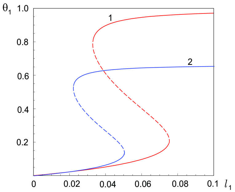
Figure 1: Adsorption isotherms of adparticles of species 1 for one-component (curve 1) and two-component (curve 2) gas for $g$ = 6, $G$ = 1, $S_{0}$ = 0.5.

The comparison of the $S-$shaped adsorption isotherms of adparticles of species 1 in Fig. 1 for one-component (curve 1) and two-component (curve 2) gas for $g=6>g_{c}$ clearly illustrate the influence of particles of species 2 in a gas mixture on the behavior of the surface coverage $\theta_{1}$. In this and subsequent figures for the surface coverages $\theta_{n}(\ell_{1})$ and the equilibrium position of oscillator $\xi(\ell_{1})$, parts of curves corresponding to stable and unstable stationary solutions are shown, respectively, by solid and broken lines.

The obtained adsorption isotherms essentially differ from the classical Langmuir isotherms. At the same, for the model taking into account variations in adsorption properties of the adsorbent in adsorption, the presence of particles of species 2 in the gas phase leads only to quantitative changes in adsorption isotherms of a one-component gas [27]: a decrease in the amount of adsorbed substance and displacement and decrease in the bistability interval of the system, which completely agrees with relations (35), (37), and (42).

As the concentration $\ell_{1}$ increases from zero, the surface coverage $\theta_{1}$ increases along the lower stable branch of the isotherm and the increment of the surface coverage is determined by both an increase in the gas concentration and a change in adsorption properties of the adsorbent due to its deformation. Since the lower stable branch of the isotherm ends at $\ell_{1}=\ell^{b}_{1,2}$, a negligible excess of the bifurcation concentration $\ell^{b}_{1,2}$ is accompanied by the jump to the upper stable branch of the isotherm, i.e., a stepwise increase in the surface coverage solely due to a change in adsorption properties of the adsorbent. This transition can include many gas particles (furthermore, of both species) successively taking part in the process of adsorption–desorption on the same adsorption site. Thus, at this stage, a certain interaction between the particle leaving the adsorption site and the particle binding with it occurs.

A subsequent increase in the concentration $\ell_{1}$ slightly affects the surface coverage $\theta_{1}$ varying along the upper stable branch because the majority of adsorption sites are already bound either with particles of species 1 or with particles of species 2.

In passing through the bifurcation concentration $\ell^{b}_{1,2}$, desorption of adparticles essentially decreases due to a considerable increase in their activation energy for desorption. As a result, for returning from the upper stable branch of the isotherm to its lower stable branch, the concentration must be lower than $\ell^{b}_{1,2}$. As the concentration $\ell_{1}$ decreases from a value greater than $\ell^{b}_{1,2}$, the surface coverage $\theta_{1}$ decreases along the upper stable branch of the isotherm up to its end at $\ell_{1}=\ell^{b}_{1,1}$. In passing through the bifurcation concentration $\ell^{b}_{1,1}$, the surface coverage jumps down to the lower stable branch of the isotherm and then decreases along this branch.

The behavior of the surface coverage $\theta_{1}$ vs $\ell_{1}$ agrees with the principle of perfect delay [36, 37]: a system, which is in a stable state at the initial time, remains in this state with variation in a parameter (the concentration $\ell_{1}$ in the case at hand) until the state exists.

According to (35), the specific features of adsorption isotherms are also true for the coordinate $\xi$ characterizing the displacement of the plane of adsorption sites from its nonperturbed position. For example, the curves in Fig. 1 also describe the equilibrium position of oscillator vs $\ell_{1}$ in adsorption of one-component and two-component gas if, instead of $\theta_{1}$, $\xi$ (for one-component adsorption) and $(2/3)\,\xi$ (for two-component adsorption) are laid off along the ordinate axis.

3.3 Equilibrium Position of Oscillator

The equilibrium position of oscillator $\xi(\ell_{1})$ is a solution of Eq. (18). To analyze solutions of this transcendental equation, we plot the function $\ell_{1}(\xi)$ inverse to the required $\xi(\ell_{1})$, i.e., the right-hand side of Eq. (18). The abscissas of the points of intersection of the graph of the function $\ell_{1}(\xi)$ with a horizontal line corresponding to the given concentration $\ell_{1}>0$ are solutions of Eq. (18). Thus, the problem under study is reduced to the investigation of the function $\ell_{1}(\xi)\geq 0$ depending on the control parameters $\,g_{1},G$, and $S_{0}$.

Points of possible finite local extrema of the function $\ell_{1}(\xi)$ are solutions of the equation

$$L(\xi;g_{1},G,S_{0})=0,$$ (51)

where

$$L(\xi;g_{1},G,S_{0})=L_{1}(\xi;g_{1})+G\,S(\xi)\,L_{2}(\xi;g_{1},G),$$ (52)

the quantity

$$L_{1}(\xi;g_{1})=1+g_{1}\xi\left(\xi-1\right)$$ (53)

is associated with adsorption of a one-component gas of species 1 and the quantity

$$L_{2}(\xi;g_{1},G)=1+g_{1}\xi\left(\xi-G\right)$$ (54)

is caused by the presence of particles of species 2 in the binary gas mixture.

In the special case where adparticles of species 2 do not affect the adsorbent deformation, $\chi_{2}=0\ (G=0)$, Eq. (45) coincides with the equation

$$L_{1}(\xi;g_{1})=0$$ (55)

for points of possible extrema of $\ell_{1}(\xi)$ in adsorption of a one-component gas of species 1.

Note that Eq. (45) is also reduced to Eq. (49) in other special case investigated in Sec. 3.2 of the identical action of all adparticles on the adsorbent, $\chi_{1}=\chi_{2}\ (G=1)$.

We denote roots of Eq. (45) for $S_{0}>0$ by $\xi^{b}_{k}$, where $k=1,2,\ldots$, and call roots $\xi^{b}_{k}$ for which the bifurcation concentrations $\ell^{b}_{1,k}=\ell_{1}(\xi^{b}_{k})>0$ bifurcation coordinates. Using (16), (17), and (45)–(48), for $G\neq 0,1$, we obtain the following relations for the bifurcation surface coverages $\theta^{b}_{1,k}=\theta_{1}(\xi^{b}_{k})$ and $\theta^{b}_{2,k}=\theta_{2}(\xi^{b}_{k})$:

$$\theta^{b}_{1,k}=\frac{L_{2}(\xi^{b}_{k};g_{1},G)}{g_{1}\left(1-G\right)},\qquad\quad\theta^{b}_{2,k}=\frac{L_{1}(\xi^{b}_{k};g_{1})}{g_{1}G\left(G-1\right)}.$$ (56)

The function $\ell_{1}(\xi)$ has a finite local extremum at the point $\xi=\xi^{b}_{k}$ if the function

$$L_{c}(\xi;g_{1},G)=2\xi-1+\left(\xi-G\right)\,L_{1}(\xi;g_{1})$$ (57)

is not equal to zero at this point. Otherwise, for

$$L_{c}(\xi^{b}_{k};g_{1},G)=0\,,$$ (58)

the investigation of $\ell_{1}(\xi)$ at this point must be continued. By $\xi^{c}_{k},\ k=1,2,3$, we denote real roots of the cubic equation (52). Both the number of these roots and their values depend on the parameters $g_{1}$ and $G$. We call roots $\xi^{c}_{k}$ for which the critical concentrations $\ell^{c}_{1,k}=\ell(\xi^{c}_{k})>0$ critical coordinates. The critical values of $S_{0}>0$ denoted by $S^{c}_{k}$ are determined from Eq. (45) for $\xi=\xi^{c}_{k}$. The critical surface coverages $\theta^{c}_{1,k}$ and $\theta^{c}_{2,k}$ are defined by relations (50) with $\xi^{b}_{k}$ replaced by $\xi^{c}_{k}$.

The more detailed analysis shows that Eq. (18) has a maximum (five-fold) multiple root for three values of the parameter $G$ equal to 2 , 1/2 , and -1 and the corresponding values of the other parameters $g_{1},\,\ell_{1},\,S_{0}$. In the four-dimensional space of control parameters $\{\ell_{1},\,S_{0},\,g_{1},\,G\}$, a point with coordinates $\ell_{1}^{\,but},\,S_{0}^{\,but},\,g_{1}^{\,but},\,G^{\,but}$ gives a five-fold stationary solution of system (7). In the three-dimensional space of solutions $\{\xi,\,\theta_{1},\,\theta_{2}\}$, this five-fold solution is a point with coordinates $\xi^{\,but},\,\theta_{1}^{\,but},\,\theta_{2}^{\,but}$. The values of three five-fold stationary solutions of system (7) and the corresponding control parameters are given in Table 1.

Table 1. Control parameters for five-fold solutions.

No.	Control parameters				Solutions
	$G^{\,but}$	$g_{1}^{\,but}$	$\ell_{1}^{\,but}$	$S_{0}^{\,but}$	$\xi^{\,but}$	$\theta_{1}^{\,but}$	$\theta_{2}^{\,but}$
1	2	3	$4\exp{(-3)}$	$\exp{(-3)}/4$	1	2/3	1/6
2	1/2	12	$\exp{(-6)}$	$4\exp{(3)}$	1/2	1/6	2/3
3	-1	3	1/4	1	0	1/6	1/6

In the general case, analysis of stationary solutions of system (7) depending on control parameters is a complicated problem. First, we decrease the dimension of the space of control parameters by fixing a value of the parameter $G$, i.e., select a three-dimensional subspace of control parameters $\{\ell_{1},\,S_{0},\,g_{1}\}$ from the original four-dimensional space. Among all three-dimensional subspaces thus obtained, there are only three subspaces for $G=2\,,1/2\,,-1$ each of which contains a unique point with coordinates $\ell_{1}^{\,but},\,S_{0}^{\,but},\,g_{1}^{\,but}$ giving a five-fold stationary solution of system (7). Moreover, in these three cases, analytic expressions are relatively simple. Then, using the results of analysis of stationary solutions of system (7) in these special cases, we can draw the corresponding conclusions for values of $G$ for which system (7) does not have five-fold stationary solutions. Since the case of negative values of $G$ is of interest in its own right, the case $G=-1$ is not investigated here. In view of the fact that the cases $G=2$ and $G=1/2$ are similar (see Table 1), below, we consider the case $G=2$.

3.4 Case $G=2$

In this case, Eq. (52) has three roots

$$\xi^{c}_{1}=1,\qquad\xi^{c}_{2}\equiv\xi^{c}_{+}=1+q,\qquad\xi^{c}_{3}\equiv\xi^{c}_{-}=1-q,\qquad q=\sqrt{1-\dfrac{3}{g_{1}}}\,,$$ (59)

which are horizontal points of inflection of the function $\ell_{1}(\xi)$ and, furthermore, at the points $\xi=\xi^{c}_{+}$ and $\xi=\xi^{c}_{-},\ d^{3}\,\ell_{1}(\xi)/d\xi^{3}\neq 0$, whereas, at the point $\xi=\xi^{c}_{1},\ d^{3}\,\ell_{1}(\xi)/d\xi^{3}\neq 0$ if $g_{1}\neq 3$ and $d^{3}\,\ell_{1}(\xi)/d\xi^{3}=d^{4}\,\ell_{1}(\xi)/d\xi^{4}=0,\ d^{5}\,\ell_{1}(\xi)/d\xi^{5}\neq 0$ if $g_{1}=3$. According to (53), the function $\ell_{1}(\xi)$ has one horizontal point of inflection $\xi^{c}_{1}$ if $g_{1}<3$ and three horizontal points of inflection if $g_{1}>3$; furthermore, only two of them ($\xi^{c}_{+}$ and $\xi^{c}_{-}$) depend on the coupling parameter $g_{1}$. This result essentially differs from results of adsorption of a one-component gas or a two-component gas for $G=1$ for which the function $\ell_{1}(\xi)$ has only one horizontal point of inflection, $\xi^{c}=1/2$, for $g_{1}=4$. If $\lim\limits_{g_{1}\rightarrow 3\,+0}\,$, then three roots (53) coalesce into one triple root.

The critical parameters $\ell^{c}_{1,k}$ and $S^{c}_{k}$ (redenoted as follows: $\ell^{c}_{1,2}\equiv\ell^{c}_{1,+},\ \ell^{c}_{1,3}\equiv\ell^{c}_{1,-},\ S^{c}_{2}\equiv S^{c}_{+},\ S^{c}_{3}\equiv S^{c}_{-}$) are equal to

$$\ell^{c}_{1,1} = 2\left(g_{1}-1\right)\,\exp{(-g_{1})},\qquad\ell^{c}_{1,\pm}=\frac{4}{g_{1}\xi^{c}_{\mp}-2}\,\exp{(-g_{1}\xi^{c}_{\pm})}\,,$$ (60)

$$S^{c}_{1} = \frac{\exp{(-g_{1})}}{2\left(g_{1}-1\right)}\,,\qquad\qquad\qquad\ S^{c}_{\pm}=\frac{g_{1}\xi^{c}_{\pm}-2}{4}\,\exp{(-g_{1}\xi^{c}_{\pm})}\,.$$ (61)

Nonnegativity of the quantities $\ell_{1}$ and $S_{0}$ imposes the following restrictions on $g_{1}$: $\ g_{1}>1$ for $\xi^{c}_{1}$ and $g_{1}\in[3,4)$ for $\xi^{c}_{\pm}$. Thus, the function $\ell_{1}(\xi)\geq 0$ has three horizontal points of inflection only for $g_{1}\in(3,4)$ and, hence, an essential difference between adsorption isotherms of two-component and one-component gases are expected precisely in this range of values of $g_{1}$. The quantities $\ell^{c}_{1,1}$, $\ell^{c}_{1,\pm}$ and $S^{c}_{1}$, $S^{c}_{\pm}$ as functions of the coupling parameter $g_{1}$ are arranged as follows: $\ell^{c}_{1,+}>\ell^{c}_{1,-}>\ell^{c}_{1,1}$ and $S^{c}_{1}>S^{c}_{+}>S^{c}_{-}$ for any $g_{1}\in(3,4)$ and coincide ($\ell^{c}_{1,1}=\ell^{c}_{1,\pm}=\ell_{1}^{\,but}\approx 0.199$ and $S^{c}_{1}=S^{c}_{\pm}=S_{0}^{\,but}\approx 0.0124$) for $g_{1}=3$.

Substituting (54) and (55) into (50), we obtain the following critical surface coverages $\theta^{c}_{n,k}$ (redenoted as follows: $\theta^{c}_{n,2}\equiv\theta^{c}_{n,+},\ \theta^{c}_{n,3}\equiv\theta^{c}_{n,-}$, where $n=1,2$):

$$\theta^{c}_{1,1}=1-\frac{1}{g_{1}},\quad\theta^{c}_{1,\pm}=\frac{2}{g_{1}},\quad\theta^{c}_{2,1}=\frac{1}{2g_{1}},\quad\theta^{c}_{2,\pm}=\frac{g_{1}\xi^{c}_{\pm}-2}{2g_{1}}\,.$$ (62)

In the degenerate case $g_{1}=3$, we have $\theta^{c}_{1,1}=\theta^{c}_{1,\pm}=\theta_{1}^{\,but}=2/3$  and  $\theta^{c}_{2,1}=\theta^{c}_{2,\pm}=\theta_{2}^{\,but}=1/6$.

In the case $g_{1}=3.5$ considered below, $\xi^{c}_{+}\approx 1.378,\ \xi^{c}_{-}\approx 0.622$ and $\ell^{c}_{1,1}\approx 0.151,\ \ell^{c}_{1,+}\approx 0.182,\ \ell^{c}_{1,-}\approx 0.161,\ S^{c}_{1}\approx 0.00604,\ S^{c}_{+}\approx 0.00568,\ S^{c}_{-}\approx 0.00502$.

The graphs of the function $\ell_{1}(\xi)$ for different values of $S_{0}$ are shown in Fig. 2. The required solutions $\xi$ of Eq. (18) are the abscissas of the points of intersection of a dashed horizontal line corresponding to the given concentration $\ell_{1}$ with the graph of the function $\ell_{1}(\xi)$.

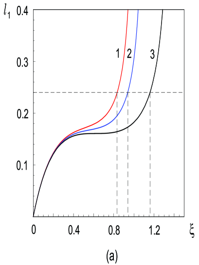
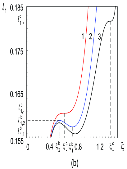
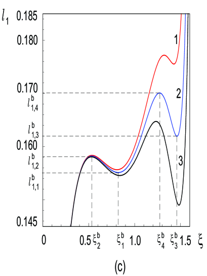
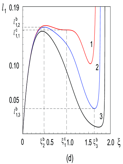
Figure 2: Graphical solution of Eq. (18) for different values of $S_{0}$: (a) $S_{0}$ = 0.001 (1), 0.003 (2), 0.005 (3); (b) $S_{0}$ = $S^{c}_{-}$ (1), 0.0055 (2), $S^{c}_{+}$ (3); (c) $S_{0}$ = 0.0057 (1), 0.00575 (2), 0.0058 (3); (d) $S_{0}$ = $S^{c}_{1}$ (1), 0.007 (2), 0.01 (3); $G=2,g_{1}=3.5$. Horizontal dashed lines correspond to constant values of the concentration $\ell_{1}$.

For low concentrations $\ell_{2}$ such that $S_{0}<S^{c}_{-}$, the curve of the function $\ell_{1}(\xi)$ intersects any horizontal line of the given concentration $\ell_{1}$ at one point, which gives a unique value of $\xi$ for any $\ell_{1}$ (Fig. 2a). An increase in $S_{0}$ is accompanied by an increase in the number of adparticles of species 2 and, hence, the adsorption-induced force acting on adsorption sites, which increases their displacement from the nonperturbed equilibrium position $\xi=0$. For the least critical $S_{0}=S^{c}_{-}$ (curve 1 in Fig. 2b), the function $\ell_{1}(\xi)$ has a horizontal point of inflection at $\xi=\xi^{c}_{-}$ and its value at this point is equal to the critical concentration $\ell^{c}_{1,-}$ ($\ell^{c}_{1,-}$ and $\xi^{c}_{-}$ are depicted in Fig. 2b). A negligible increase in $S_{0}$ leads to the deformation of the curve in the neighborhood of the point $\xi^{c}_{-}$ so that there appear a minimum and a maximum of the function $\ell_{1}(\xi)$ equal to the bifurcation concentrations $\ell^{b}_{1,1}$ and $\ell^{b}_{1,2}$ ($\ell^{b}_{1,1}<\ell^{b}_{1,2}<\ell^{c}_{1,-}$), respectively, at the points $\xi=\xi^{b}_{1}$ and $\xi=\xi^{b}_{2}$. As $S_{0}$ increases, the bifurcation concentrations $\ell^{b}_{1,1}$ and $\ell^{b}_{1,2}$ decrease and the width $I_{2,1}=\ell^{b}_{1,2}-\ell^{b}_{1,1}$ of the interval $[\ell^{b}_{1,1},\,\ell^{b}_{1,2}]$ called the first bistability interval of the system increases (cf. $I_{2,1}$ for curves 2 and 3 in Fig. 2b). In Fig. 2b, the bifurcation concentrations $\ell^{b}_{1,1}$ and $\ell^{b}_{1,2}$ and the bifurcation coordinates $\xi^{b}_{1}$ and $\xi^{b}_{2}$ are shown for $S_{0}=0.0055$, $S_{0}\in(S^{c}_{-},\,S^{c}_{+})$. The situation is similar to that in adsorption of a one-component gas [27] or a two-component gas for $G=1$ if values of the coupling parameter are greater than critical: For $\ell_{1}\notin[\ell^{b}_{1,1},\,\ell^{b}_{1,2}]$, there is a single-valued correspondence between the concentration $\ell_{1}$ and the coordinate $\xi$; for any $\ell_{1}\in(\ell^{b}_{1,1},\,\ell^{b}_{1,2})$, there are three values of the coordinate $\xi$:  $\xi_{1}<\xi_{2}<\xi_{3}$; furthermore, the stationary solutions $\xi_{1}$ and $\xi_{3}$ of system (7) are asymptotically stable and the stationary solution $\xi_{2}$ is unstable. If the concentration $\ell_{1}\in[\ell^{b}_{1,1},\,\ell^{b}_{1,2}]$ tends to the end point $\ell^{b}_{1,1}$ (or $\ell^{b}_{1,2}$) of the interval, then the stable $\xi_{3}$ (or $\xi_{1}$) and unstable $\xi_{2}$ solutions approach each other and, in the limit $\ell_{1}=\ell^{b}_{1,1}$ (or $\ell_{1}=\ell^{b}_{1,2}$), coalesce into the two-fold solution $\xi^{b}_{1}$ (or $\xi^{b}_{2}$). Thus, for $S_{0}\in(S^{c}_{-},\,S^{c}_{+})$, the system is monostable if $\ell_{1}\notin[\ell^{b}_{1,1},\,\ell^{b}_{1,2}]$ and bistable if $\ell_{1}\in[\ell^{b}_{1,1},\,\ell^{b}_{1,2}]$.

For the second critical value $S_{0}=S^{c}_{+}$ (curve 3 in Fig. 2b), the function $\ell_{1}(\xi)$ has a horizontal point of inflection at $\xi=\xi^{c}_{+}$ and its value at this point is equal to the maximum critical concentration $\ell^{c}_{1,+}$ ($\ell^{c}_{1,+}$ and $\xi^{c}_{+}$ are shown in Fig. 2b). As $S_{0}\in(S^{c}_{+},\,S^{c}_{1})$ increases, the behavior of the function $\ell_{1}(\xi)$ (Fig. 2c) is similar to that in Fig. 2b for $S_{0}\in(S^{c}_{-},\,S^{c}_{+})$. First, the function changes the shape in the neighborhood of the point $\xi^{c}_{+}$ so that $\ell_{1}(\xi)$ has a minimum and a maximum equal to the bifurcation concentrations $\ell^{b}_{1,3}$ and $\ell^{b}_{1,4}$ ($\ell^{b}_{1,3}<\ell^{b}_{1,4}<\ell^{c}_{1,+}$), respectively, at the points $\xi=\xi^{b}_{3}$ and $\xi=\xi^{b}_{4}$. This yields the second bistability interval $[\ell^{b}_{1,3},\,\ell^{b}_{1,4}]$ of the system of width $I_{4,3}=\ell^{b}_{1,4}-\ell^{b}_{1,3}$ nonintersecting with the first. As $S_{0}$ increases, the bifurcation concentrations $\ell^{b}_{1,3}$ and $\ell^{b}_{1,4}$ decrease and the width $I_{4,3}$ increases (cf. $I_{4,3}$ for the curves in Fig. 2c). The bifurcation concentrations $\ell^{b}_{1,1}$, $\ell^{b}_{1,2}$ for the first bistability interval and $\ell^{b}_{1,3},\ell^{b}_{1,4}$ for the second and the bifurcation coordinates $\xi^{b}_{1},\xi^{b}_{2}$ and $\xi^{b}_{3},\xi^{b}_{4}$ for them are shown in Fig. 2c for $S_{0}=0.00575$, $S_{0}\in(S^{c}_{+},\,S^{c}_{1})$. An increase in $S_{0}\in(S^{c}_{+},\,S^{c}_{1})$ leads, first, to the partial overlapping of the first and second bistability intervals and then to their complete overlapping where the second bistability interval includes the first (curve 3 in Fig. 2c). In the case of the overlapping bistability intervals, for any concentration $\ell_{1}\in(\ell^{t}_{1,1},\,\ell^{t}_{1,2})$, where $[\ell^{t}_{1,1},\,\ell^{t}_{1,2}]=[\ell^{b}_{1,1},\,\ell^{b}_{1,2}]\cap[\ell^{b}_{1,3},\,\ell^{b}_{1,4}]$, $\ell^{t}_{1,1}=\max\,(\ell^{b}_{1,1},\,\ell^{b}_{1,3})$, $\ell^{t}_{1,2}=\min\,(\ell^{b}_{1,2},\,\ell^{b}_{1,4})$, there are five values of the coordinate $\xi$:  $\xi_{1}<\xi_{2}<\xi_{3}<\xi_{4}<\xi_{5}$; furthermore, the stationary solutions $\xi_{1}$, $\xi_{3}$, and $\xi_{5}$ of system (7) are asymptotically stable and the stationary solutions $\xi_{2}$ and $\xi_{4}$ are unstable. Thus, for $\ell_{1}\in[\ell^{t}_{1,1},\,\ell^{t}_{1,2}]$, the system is tristable. We call the concentration interval $[\ell^{t}_{1,1},\,\ell^{t}_{1,2}]$ a tristability interval of the system.

If the concentration $\ell_{1}\in[\ell^{t}_{1,1},\,\ell^{t}_{1,2}]$ tends to the end point of the interval, then a stable solution and an unstable solution approach each other and, in the limit $\ell_{1}=\ell^{t}_{1,1}$ (or $\ell_{1}=\ell^{t}_{1,2}$), coalesce into a two-fold solution. In this case, system (7) has four stationary solutions (two asymptotically stable, one unstable, and one two-fold). For $\ell_{1}=\ell^{t}_{1,1}$, the two-fold solution is $\xi^{b}_{1}$ if $\ell^{b}_{1,1}>\ell^{b}_{1,3}$ or $\xi^{b}_{3}$ if $\ell^{b}_{1,1}<\ell^{b}_{1,3}$. For $\ell_{1}=\ell^{t}_{1,2}$, the two-fold solution is $\xi^{b}_{2}$ if $\ell^{b}_{1,2}<\ell^{b}_{1,4}$ or $\xi^{b}_{4}$ if $\ell^{b}_{1,2}>\ell^{b}_{1,4}$.

The arguments for a two-fold solution for the end points of the tristability interval must be corrected for two values of $S_{0}\in(S^{c}_{+},\,S^{c}_{1})$ denoted by $S_{d}$ and $S_{t}$ and corresponding, respectively, to the equality of the lower (for $S_{0}=S_{d}\approx 0.00578$) or upper (for $S_{0}=S_{t}\approx 0.00589$) end points of the bistability intervals, i.e., the cases of equal minima $\ell^{b}_{1,1}=\ell^{b}_{1,3}\equiv\ell^{b}_{d}\approx 0.155$ ($\ell^{t}_{1,1}=\ell^{b}_{d}$) or maxima $\ell^{b}_{1,2}=\ell^{b}_{1,4}\equiv\ell^{b}_{t}\approx 0.158$ ($\ell^{t}_{1,2}=\ell^{b}_{t}$) of the function $\ell_{1}(\xi)$. For $\ell^{t}_{1,1}=\ell^{b}_{d}$ (or $\ell^{t}_{1,2}=\ell^{b}_{t}$), if the concentration $\ell_{1}\in[\ell^{t}_{1,1},\ell^{t}_{1,2}]$ tends to the end point $\ell^{b}_{d}$ (or $\ell^{b}_{t}$) of the interval, then simultaneously two pairs of stable and unstable solutions approach each other and, in the limit $\ell_{1}=\ell^{b}_{d}$ (or $\ell_{1}=\ell^{b}_{t}$), coalesce into two two-fold solutions. In these two cases, system (7) has three stationary solutions (one asymptotically stable and two two-fold). As soon as the concentration $\ell_{1}$ leaves the tristability interval, both two-fold solutions disappear and the system becomes monostable.

It is worth noting one more case where system (7) has one asymptotically stable and two two-fold stationary solutions. This case occurs for the value of $S_{0}\in(S^{c}_{+},\,S^{c}_{1})$ denoted by $S_{u}$ ($S_{u}\approx 0.005764$) for which two bistability intervals have only one common point $\ell^{b}_{u}$ such that $\ell^{b}_{1,2}=\ell^{b}_{1,3}\equiv\ell^{b}_{u}\approx 0.1582$, i.e., the maximum of $\ell_{1}(\xi)$ at $\xi=\xi^{b}_{2}$ is equal to the minimum of this function at $\xi=\xi^{b}_{3}$: $\ell_{1}(\xi^{b}_{2})=\ell_{1}(\xi^{b}_{3})\equiv\ell^{b}_{u}$. Unlike the cases considered above for two-fold solutions, in this case, a negligible variation (furthermore, in any side) in $\ell_{1}$ from $\ell^{b}_{u}$ is accompanied by the disappearance of one two-fold solution and split of the second into two (stable and unstable) solutions.

Three values $S_{d}$, $S_{t}$, and $S_{u}$ of the parameter $S_{0}\in(S^{c}_{+},\,S^{c}_{1})$ for which the system has two two-fold solutions are arranged as follows: $S_{t}>S_{d}>S_{u}$.

As $S_{0}\in(S^{c}_{+},\,S^{c}_{1})$ increases, the first bistability interval decreases and the points $\xi^{b}_{1}$ and $\xi^{b}_{4}$ at which the function $\ell_{1}(\xi)$ has the minimum and the maximum, respectively, approach each other. For $S_{0}=S^{c}_{1}$, the points coalesce into one $\xi^{c}_{1}$ at which the function $\ell_{1}(\xi)$ has a horizontal point of inflection and is equal to the least critical concentration $\ell^{c}_{1,1}$ (curve 1 in Fig. 2d). For $S_{0}>S^{c}_{1}$, the inflection of the function $\ell_{1}(\xi)$ disappears and the function has one minimum and one maximum at the points $\xi=\xi^{b}_{3}$ and $\xi=\xi^{b}_{2}$, respectively (curves 2 and 3 in Fig. 2d). Thus, for $S_{0}>S^{c}_{1}$, the system has only one bistability interval $[\ell^{b}_{1,3},\,\ell^{b}_{1,2}]$ of width $I_{2,3}=\ell^{b}_{1,2}-\ell^{b}_{1,3}$. The bifurcation concentrations $\ell^{b}_{1,3}$ and $\ell^{b}_{1,2}$ and the corresponding bifurcation coordinates $\xi^{b}_{3}$ and $\xi^{b}_{2}$ are shown in Fig. 2d for $S_{0}=0.007>S^{c}_{1}$.

Figure 3: Dependence of the critical concentrations $\ell^{c}_{1,+}$ (curve 1), $\ell^{c}_{1,-}$ (curve 2), and $\ell^{c}_{1,1}$ (curve 3) on the coupling parameter $g_{1}$ for $G$ = 2.

Thus, to investigate specific features of stationary solutions of system (7), first, it is necessary to determine the critical values of $S_{0}$ for which the function $\ell_{1}(\xi)$ has horizontal points of inflection and the critical concentrations at these points. The critical concentration $\ell_{1}^{c}$ and parameter $S_{0}$ as functions of the coupling parameter $g_{1}$ defined by relations (54) and (55) are shown in Figs. 3 and 4, respectively, in the range of values of $g_{1}$ where the function $\ell_{1}(\xi)\geq 0$ has three horizontal points of inflection.

Note that the behavior of the function $\ell_{1}(\xi)$ shown in Fig. 2 for $g_{1}=3.5$ remains true for other values of $g_{1}\in(3,\,4)$. Thus, qualitative analysis of specific features of stationary solutions of system (7) can be made using the graphs in Fig. 2 and the curves for the critical parameters $\ell_{1}$ and $S_{0}$ in Figs. 3 and 4.

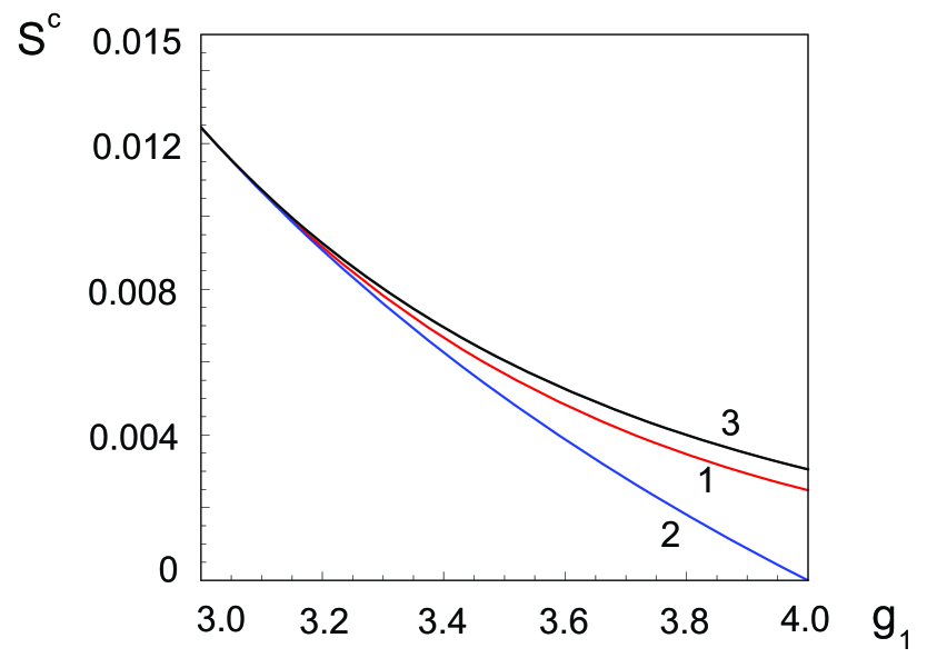
Figure 4: Dependence of $S^{c}_{+}$ (curve 1), $S^{c}_{-}$ (curve 2) and $S^{c}_{1}$ (curve 3) on the coupling parameter $g_{1}$ for $G$ = 2.

Specific features of the behavior of system (7) for $G=2$ can be clearly illustrated by plotting a bifurcation surface, which is a set of multiple roots of Eq. (18), in the three-dimensional space of control parameters $\{\ell_{1},\,S_{0},\,g_{1}\}$. Instead of this surface, we plot the bifurcation curve $\ell_{1}(S_{0})$, which is the projection of the section of this bifurcation surface by a plane of a fixed value of the coupling parameter $g_{1}$ onto the plane ($S_{0},\,\ell_{1}$). To this end, using relations (18) and (45), we obtain the following representation of this bifurcation curve in the parametric form, which is true for any $G\neq 0,1$:

$$S_{0}=-\frac{1}{G}\,\frac{L_{1}(\xi;g_{1})}{L_{2}(\xi;g_{1},G)}\,\frac{1}{w(\xi)}\,,\qquad\ell_{1}=\frac{G}{1-G}\,\frac{L_{2}(\xi;g_{1},G)\,\exp{(-g_{1}\xi)}}{1+g_{1}(1-\xi)(G-\xi)}\,.$$ (63)

The bifurcation curve in Fig. 5 plotted for the same values of $g_{1}$ and $G$ as in Fig. 2 has several singular points, which are shown in Fig. 5b where a part of the curve is scaled up for the most interesting range $S_{0}\in(S^{c}_{-},S^{c}_{1}$), $\ell_{1}\in(\ell^{c}_{1,1},\ell^{c}_{1,+})$. The points $P_{1}\equiv(S^{c}_{1},\,\ell^{c}_{1,1}),\ P_{+}\equiv(S^{c}_{+},\,\ell^{c}_{1,+})$, and $P_{-}\equiv(S^{c}_{-},\,\ell^{c}_{1,-})$ are the cusps of the bifurcation curve corresponding to the horizontal points of inflection of the function $\ell_{1}(\xi)$ at $\xi=\xi^{c}_{1},\ \xi^{c}_{+}$, and $\xi^{c}_{-}$, respectively. The self-intersection points of the bifurcation curve $P_{d}\equiv(S_{d},\,\ell^{b}_{d}),\ P_{t}\equiv(S_{t},\,\ell^{b}_{t})$, and $P_{u}\equiv(S_{u},\,\ell^{b}_{u})$ correspond to the system with two two-fold stationary solutions. For any point of the first quadrant of this plane lying outside the bifurcation curve, system (7) has one asymptotically stable stationary solution, i.e., it is a domain of monostability of the system. For a point lying in the curvilinear quadrangle $P_{t}\,P_{u}\,P_{d}\,P_{1}$, which is the domain of intersection of two curvilinear triangles $P_{1}\,P_{+}\,P_{d}$ and $P_{1}\,P_{-}\,P_{t}$, system (7) has five stationary solutions (three asymptotically stable and two unstable), i.e., it is the domain of tristability of the system. If a point lies in one of the domains: the curvilinear triangles $P_{t}\,P_{+}\,P_{u}$ and $P_{u}\,P_{-}\,P_{d}$ and the domain $B_{t}\,P_{t}\,P_{1}\,P_{d}\,B_{d}$ ($B_{t}$ and $B_{d}$ are symbolic notations for points of the upper and lower branches of the bifurcation curve, respectively, in the limit $S_{0}\rightarrow\infty$), then system (7) has three stationary solutions (two asymptotically stable and one unstable), i.e., they are domains of bistability of the system. At any point of the bifurcation curve, except for the points of the boundary of the curvilinear quadrangle $P_{t}\,P_{u}\,P_{d}\,P_{1}$ and the singular points $P_{+}$ and $P_{-}$, system (7) has two stationary solutions (one asymptotically stable and one two-fold). At a non vertex point of the boundary of the quadrangle $P_{t}\,P_{u}\,P_{d}\,P_{1}$, system (7) has four stationary solutions (three structurally stable (furthermore, two asymptotically stable and one unstable) and one two-fold). At the singular points $P_{d},\ P_{t}$, and $P_{u}$, system (7) has three stationary solutions (one asymptotically stable and two two-fold). At the singular points $P_{+}$ and $P_{-}$, system (7) has one three-fold stationary solution. At the singular point $P_{1}$, system (7) has three stationary solutions (two asymptotically stable and one three-fold).

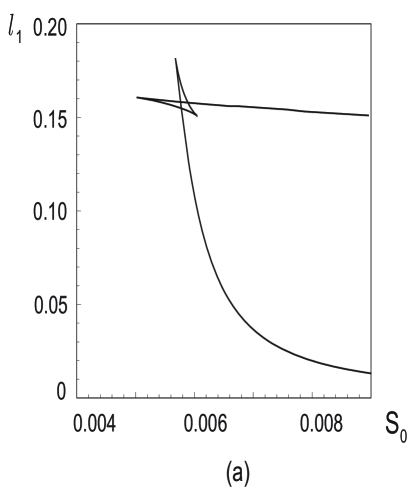
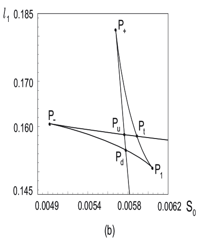
Figure 5: Bifurcation curve for $G=2,g_{1}=3.5$.

Motion in the plane of control parameters ($S_{0},\,\ell_{1}$) along a line can be accompanied by the appearance of new solutions, disappearance of existing solutions, and a change in solution stability in intersecting the bifurcation curve. This depends on both the point of intersection and the line itself if it intersects the bifurcation curve at a singular point and the direction of motion. Independently of the line, its intersection with the bifurcation curve at a nonsingular point is accompanied by the appearance/disappearance (depending on the direction of motion) of a pair of stationary (stable and unstable) solutions of system (7). In entering the domain $P_{t}\,P_{+}\,P_{u}$ or $P_{u}\,P_{-}\,P_{d}$ through the cusp $P_{+}$ or $P_{-}$ , respectively, a stable solution splits into three solutions (two stable and one unstable) and changes its stability. In entering the domain $P_{t}\,P_{+}\,P_{u}$ $P_{1}$ through the cusp $P_{1}$, an unstable solution splits into three solutions (two unstable and one stable). In leaving these domains along a line passing through the cusp, three solutions (two stable and one unstable in the domains $P_{t}\,P_{+}\,P_{u}$ and $P_{u}\,P_{-}\,P_{d}$ or two unstable and one stable in the domain $P_{t}\,P_{+}\,P_{u}$ $P_{1}$) coalesce into a three-fold solution at the cusp with its subsequent transformation outside the point into a simple stable (for the points $P_{+}$ and $P_{-}$) or unstable (for the point $P_{1}$) solution. In entering/leaving the domain of tristability $P_{t}\,P_{u}\,P_{d}\,P_{1}$ from/for the domain of monostability through the points $P_{d}$, $P_{t}$, or $P_{u}$, which are unique common points of these domains, two two-fold solutions simultaneously appear/disappear. If a line enters the domain $P_{t}\,P_{+}\,P_{u}$ from the domain $P_{u}\,P_{-}\,P_{d}$ (or, conversely, enters the domain $P_{u}\,P_{-}\,P_{d}$ from the domain $P_{t}\,P_{+}\,P_{u}$) through their common point $P_{u}$, then a stable solution and an unstable solution coalesce into a two-fold solution at the point $P_{u}$ that disappears with moving away from the point, whereas another two-fold solution appears at this point and then splits into a pair of stable and unstable solutions. A similar behavior of the system occurs in the motion from one domain of bistability to another through their common point ($P_{d}$ for the domains of bistability $P_{u}\,P_{-}\,P_{d}$ and $B_{t}\,P_{t}\,P_{1}\,P_{d}\,B_{d}$ or $P_{t}$ for the domains of bistability $P_{t}\,P_{+}\,P_{u}$ and $B_{t}\,P_{t}\,P_{1}\,P_{d}\,B_{d}$).

The bifurcation curve for other values of the coupling parameter $g_{1}\in(3,\,4)$ is similar to the curve in Fig. 5. As $g_{1}$ decreases, the triangles $P_{u}\,P_{-}\,P_{d}$ and $P_{t}\,P_{+}\,P_{u}$ and the quadrangle, $P_{t}\,P_{u}\,P_{d}\,P_{1}$ decrease and, in the limit $g_{1}\rightarrow 3$, shrink to the point $P_{\,but}\equiv(S_{0}^{\,but},\,\ell_{1}^{\,but}$), and tristability of the system is impossible for $g_{1}\leq 3$. As $g_{1}$ increases, the triangles $P_{u}\,P_{-}\,P_{d}$ and $P_{t}\,P_{+}\,P_{u}$ elongate toward the ordinate axis and along it, respectively, and, furthermore, in the limit $g_{1}\rightarrow 4$, the vertex $P_{-}$ of the triangle $P_{u}\,P_{-}\,P_{d}$ lies on the ordinate axis ($P_{-}\equiv(0,\ell_{1}^{c}$), where $\ell_{1}^{c}=\exp{(-2)}$ is the critical concentration in adsorption of a one-component gas of species 1, and the vertex $P_{+}$ of the triangle $P_{t}\,P_{+}\,P_{u}$ is at infinity ($P_{+}\equiv(\exp{(-6)},\infty$).

The graphs of the equilibrium position of oscillator $\xi(\ell_{1})$ and the surface coverage $\theta_{n}(\ell_{1})$ in Figs. 6 and 7, respectively, plotted on the basis of relations (16)–(20) clearly illustrate their essential dependence on the value of $S_{0}$. In the most interesting range $S_{0}\in(S^{c}_{-},\,S^{c}_{1})$ (Figs. 6b–h and 7b–h), these characteristics are shown only in a small interval of the concentration $\ell_{1}$ in which the adsorption isotherms essentially differ from the classical Langmuir ones.

For $S_{0}<S^{c}_{-}$, the coordinate $\xi$ increases with the concentration $\ell_{1}$ and tends to its asymptotic value $\xi^{a}$ determined from Eq. (25) (Fig. 6a). According to analysis in Sec. 3.1, $\xi^{a}\in(1,2)$; the numerical analysis shows that $\xi^{a}$ increases with $S_{0}$. The adsorption isotherms in Fig. 7a are similar to the classical Langmuir isotherms. However, unlike the Langmuir case for which the ratio $\theta_{2}/\theta_{1}$ is the constant equal to $S_{0}$, variations in adsorption properties of the adsorbent in the competitive adsorption leads to the dependence of this ratio on the concentration $\ell_{1}$. As $\ell_{1}$ increases, the ratio $\theta_{2}/\theta_{1}$ increases and considerably exceeds the Langmuir one (for large values of $\ell_{1}$, approximately by a factor of 50).

For $S_{0}\in(S^{c}_{-},\,S^{c}_{+})$, the coordinate $\xi(\ell_{1})$ (Fig. 6b) and the surface coverage $\theta_{n}(\ell_{1})$ (Fig. 7b) have a hysteresis in the first bistability interval of the system.

As the concentration $\ell_{1}$ increases from zero, both the coordinate $\xi$ and the surface coverages $\theta_{n}$ increase along their lower stable branches ending at the bifurcation concentration $\ell_{1}=\ell^{b}_{1,2}$. At this concentration, $\xi$ and $\theta_{n}$ jump up to their upper stable branches solely due to a change in adsorption properties of the adsorbent. For convenience, transitions between stable branches of $\xi(\ell_{1})$ are shown in Fig. 6 by light vertical lines with arrows indicating the direction of transition. Arrows under and above stable branches of $\xi(\ell_{1})$ indicate the direction of variation in $\ell_{1}$. As the concentration $\ell_{1}$ increases from $\ell^{b}_{1,2}$, the coordinate $\xi$ and the surface coverages $\theta_{n}$ increase along the upper stable branches and tend to their asymptotic values $\xi^{a}$ and $\theta^{a}_{n}$ defined by relations (25) and (24), respectively.

The transition of the coordinate $\xi$ from the lower stable branch to the upper one at the bifurcation concentration $\ell^{b}_{1,2}$ is accompanied by an increase in the activation energy for desorption of adparticles, which hampers their desorption. As a result, as the concentration $\ell_{1}$ decreases from a value greater than $\ell^{b}_{1,2}$, the reverse transition of $\xi$ and $\theta_{n}$ from their upper stable branches to the lower ones occurs at the lower bifurcation concentration $\ell^{b}_{1,1}<\ell^{b}_{1,2}$.

The curves in Figs. 6c and 7c correspond to the special case $S_{0}=S_{u}$ where the system has two bistability intervals with common point $\ell_{1}=\ell^{b}_{u}$. Each of the functions $\xi(\ell_{1})$ and $\theta_{n}(\ell_{1})$ has three stable and two unstable branches (the $j$th unstable branch connects the $j$th and $(j+1)$th stable branches, where $j=1,2$). However, the behaviors of these functions are different. The coordinate $\xi(\ell_{1})$ has two successive hystereses in the touching bistability intervals (Fig. 6c). As the concentration $\ell_{1}$ increases from zero, the coordinate $\xi$ increases along the first stable branch up to its end at $\ell_{1}=\ell^{b}_{u}$; then jumps up to the second stable branch and increases with $\ell_{1}$ along this branch up to its end at $\ell_{1}=\ell^{b}_{1,4}$; then jumps up to the third stable branch and increases along it with $\ell_{1}$ tending to its asymptotic value $\xi^{a}$. As the concentration $\ell_{1}$ decreases from a value greater than $\ell^{b}_{1,4}$, the coordinate $\xi$ successively jumps down from the third stable branch to the second and from the second stable branch to the first, respectively, at the bifurcation concentrations $\ell^{b}_{u}$ and $\ell^{b}_{1,1}$ at which these branches end, furthermore, the transitions from the first and third stable branches to the second go along the same vertical straight line $\ell_{1}=\ell^{b}_{u}$.

The behavior of the surface coverage $\theta_{2}(\ell_{1})$ in Fig. 7c is similar to the behavior of the coordinate $\xi(\ell_{1})$ in Fig. 6c. Note that a similar behavior of $\theta_{2}(\ell_{1})$ and $\xi(\ell_{1})$ also occurs for other values of $S_{0}$ (cf. curve 2 in Fig. 7c–i with curve in Fig. 6c–i).

The surface coverage $\theta_{1}(\ell_{1})$ has another behavior (curve 1 in Fig. 7c). The different location of the second and third stable branches of $\theta_{1}(\ell_{1})$ and $\theta_{2}(\ell_{1})$ illustrates the essentially different behavior of the surface coverages $\theta_{1}$ and $\theta_{2}$ in transition between stable branches at bifurcation concentrations of $\ell_{1}$. The transition of the surface coverages $\theta_{n}$ from the first stable branch to the second leads to their stepwise increase. However, in transition of the surface coverages $\theta_{n}$ from the second stable branch to the third, the value of $\theta_{2}$ stepwise increases, whereas the value of $\theta_{1}$ stepwise decreases. Thus, as the concentration $\ell_{1}$ increases, the surface coverage $\theta_{2}$ continuously increases with $\ell_{1}$ along its stable branches and stepwise increases in transition between stable branches at a bifurcation concentration of $\ell_{1}$, whereas the surface coverage $\theta_{1}$ can continuously both increase and decrease with $\ell_{1}$ along its stable branches and stepwise both increase and decrease in transition between stable branches at a bifurcation concentration of $\ell_{1}$. This different behavior of the surface coverages $\theta_{1}(\ell_{1})$ and $\theta_{2}(\ell_{1})$ is caused by the different growth of the residence times of adparticles of different species on the deformable adsorbent in adsorption and, furthermore, quantity (14) characterizing this difference exponentially increases with displacement of adsorption sites from their nonperturbed equilibrium position. This leads to a greater amount of adparticles of species 2 relative to that of species 1 (cf. the third stable branches of the surfaces coverages $\theta_{1}(\ell_{1})$ and $\theta_{2}(\ell_{1})$), whereas, in the classical case, $\theta_{2}\ll\theta_{1}$. This result agrees with condition (28) according to which, for $\xi^{a}>1.5$, the asymptotic ratio $S(\xi^{a})$ defined by relation (27) is greater than 1. Indeed, in the considered case, $\xi^{a}\approx 1.65$, which yields $S(\xi^{a})\approx 1.85$.

One more specific feature is a self-tangency point of $\theta_{1}(\ell_{1})$ (point of contact of four branches of the function: two stable (first and third) and two unstable branches) at $\ell_{1}=\ell^{b}_{u}$. As was discussed above, in this special case, there are three stationary coordinates: two two-fold $\xi^{b}_{2}$ and $\xi^{b}_{3}$, $\xi^{b}_{2}<\xi^{b}_{3}$, and one stable lying between them and equal to the ordinate of the point of intersection of the second stable branch of $\xi(\ell_{1})$ with the vertical straight line $\ell_{1}=\ell^{b}_{u}$ (Fig. 6c). Taking into account the principle of perfect delay [36, 37] and the condition for transition between stationary solutions of the system (according to which all components ($\xi$, $\theta_{1}$, and $\theta_{2}$) of a stationary three-component solution simultaneously go from their stable branches at a bifurcation concentration at which these branches end to the corresponding other stable branches), as $\ell_{1}$ increases, a discontinuous transition of $\theta_{1}$ to the second stable branch occurs at $\ell_{1}=\ell^{b}_{u}$ rather than a continuous transition to the third stable branch touching with the first stable branch at $\ell_{1}=\ell^{b}_{u}$. Further, as $\ell_{1}$ increases, the surface coverage $\theta_{1}$ decreases along the second stable branch up to its end at $\ell_{1}=\ell^{b}_{1,4}$; then jumps down to the third stable branch and decreases along this branch tending to its asymptotic value $\theta^{a}_{1}$. As the concentration $\ell_{1}$ decreases from a value greater than $\ell^{b}_{1,4}$, the surface coverage $\theta_{1}$ varies along the third stable branch up to its end at $\ell_{1}=\ell^{b}_{u}$; then jumps up to the second stable branch, furthermore, along the same vertical straight line as for increasing $\ell_{1}$, rather than continuously goes to the first stable branch touching with the second stable branch at $\ell_{1}=\ell^{b}_{u}$, and then varies along the second stable branch up to its end at $\ell_{1}=\ell^{b}_{1,1}$; then jumps down to the first stable branch and decreases along this branch.

It turns out that the equality of two bifurcation values of the surface coverage $\theta_{1}$ for $\ell_{1}=\ell^{b}_{u}$ and $S_{0}=S_{u}\$ ($\theta^{b}_{1,2}=\theta^{b}_{1,3}\equiv\theta^{u}_{1}$) shown in Fig. 7c also occurs for other values of the parameters $g_{1}$ and $G$; the values of $\ell^{b}_{u}$ and $S_{u}$ depend on $g_{1}$ and $G$. Using relations (50) and (48), we obtain that, in this case, the bifurcation coordinates $\xi^{b}_{2}$ and $\xi^{b}_{3}$ are symmetrically located about $G/2$: $\ \xi^{b}_{2}=G/2-\eta$ and $\xi^{b}_{3}=G/2+\eta$. For $G=2$, the quantity $\eta$ is a solution the equation

$$\frac{g_{1}\eta}{1+g_{1}\eta^{2}}=\tanh{g_{1}\eta}\,,$$ (64)

the quantities $S_{u}$ and $\ell^{b}_{u}$ are expressed in terms of $\eta$ as follows:

$$S_{u}=\frac{\cosh{g_{1}\eta}}{\cosh{2g_{1}\eta}}\,\frac{\eta\,(1-\eta\,\tanh{g_{1}\eta})}{(1+\eta^{2})\,\tanh{2g_{1}\eta}-2\eta}\,\exp{(-g_{1})}\,,\quad\ell^{b}_{u}=2\,\frac{g_{1}(1-\eta^{2})-1}{1+g_{1}\eta(1+\eta)}\,\exp{(g_{1}(\eta-1))}\,,$$ (65)

and the bifurcation surface coverages have the form

$$\theta^{u}_{1}=1-\eta^{2}-\frac{1}{g_{1}}\,,\qquad\theta^{b}_{2,2}=\frac{1}{2}\,\biggl{\{}\frac{1}{g_{1}}+\eta\left(\eta-1\right)\biggr{\}}\,,\quad\theta^{b}_{2,3}=\frac{1}{2}\,\biggl{\{}\frac{1}{g_{1}}+\eta\left(\eta+1\right)\biggr{\}}\,.$$ (66)

Equation (58) has a nonzero solution $\eta$ for $g_{1}>3$ and its value increases with $g_{1}$: $\eta\in(0,1)$ for $g_{1}\in(3,\infty)$. According to (60), as $g_{1}$ increases, the difference $\delta^{u}=\theta^{u}_{1}-\theta^{b}_{2,3}$ decreases from the maximum value $\lim\limits_{g_{1}\rightarrow 3}\delta^{u}=0.5$ to the minimum value $\lim\limits_{g_{1}\rightarrow\infty}\delta^{u}=-1$. For example, $\delta^{u}\approx 0.453$ for $g_{1}=3.01$ and $\delta^{u}\approx-0.774$ for $g_{1}=10$. For $g_{1}=3.5$ (Figs. 6c and 7c), $\eta\approx 0.468$ and the values of $\theta^{u}_{1}$ and $\theta^{b}_{2,3}$ are close to each other ($\delta^{u}\approx 0.01$).

The curves in Figs. 6d–h and 7d–h correspond to different cases of tristability of the system: partial (Figs. 6d,h and 7d,h) and complete (Figs. 6e–g and 7e–g) overlapping of the bistability intervals $[\ell^{b}_{1,1},\,\ell^{b}_{1,2}]$ and $[\ell^{b}_{1,3},\,\ell^{b}_{1,4}]$. In the domain $\ell_{1}\in[\ell^{t}_{1,1},\,\ell^{t}_{1,2}]$, the coordinate $\xi(\ell_{1})$ and the surface coverage $\theta_{2}(\ell_{1})$ have two “parallel” hystereses.

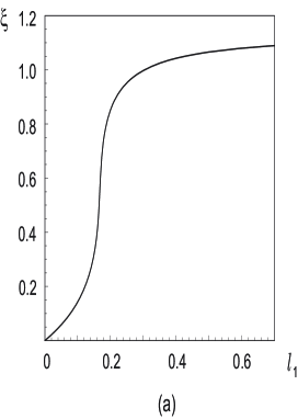
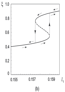
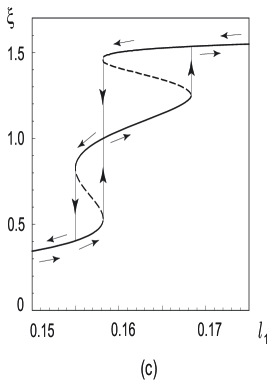
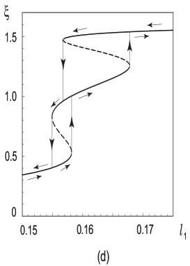
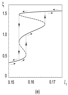
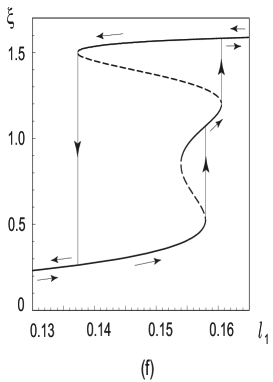
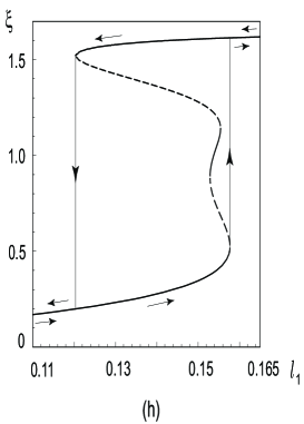
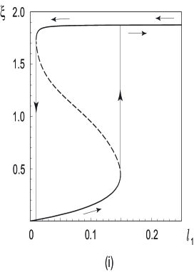
Figure 6: Equilibrium position of oscillator $\xi$ vs the concentration $\ell_{1}$ for different values of $S_{0}$: $S_{0}$ = 0.003 (a), 0.0055 (b), $S_{u}$ (c), 0.00577 (d), $S_{d}$ (e), 0.00585 (f), $S_{t}$ (g), 0.00593 (h), 0.01 (i); $G=2,g_{1}=3.5$.

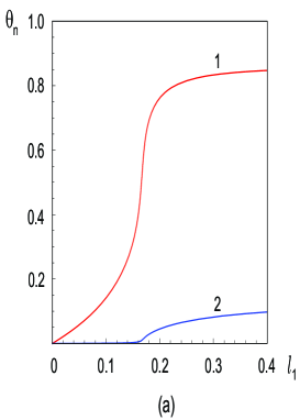
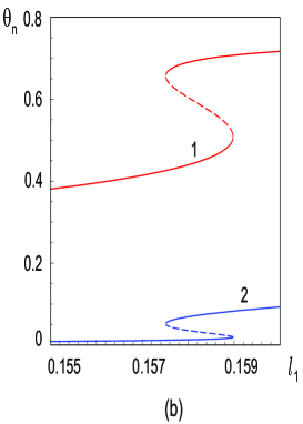
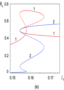
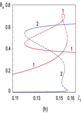
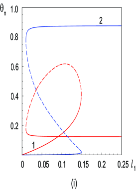
Figure 7: Surface coverages $\theta_{n}$ by adparticles of species $n$ ($n=1$, curve 1; $n=2$, curve 2) vs the concentration $\ell_{1}$. The values of $S_{0},G$, and $g_{1}$ are the same as in Fig. 6.

As the concentration $\ell_{1}$ increases/decreases, the behavior of $\xi(\ell_{1})$ in Fig. 6d is similar to the behavior of this function in Fig. 6c but the transitions of $\xi$ from the second (as $\ell_{1}$ increases) and third (as $\ell_{1}$ decreases) stable branches to the second stable branch go along the different vertical straight lines $\ell_{1}=\ell^{b}_{1,2}$ and $\ell_{1}=\ell^{b}_{1,3}$ rather than the same one as in Fig. 6c.

The behavior of the surface coverage $\theta_{1}(\ell_{1})$ in Fig. 7d is similar to its behavior in Fig. 7c but with the replacement of the self-tangency point of $\theta_{1}(\ell_{1})$ in Fig. 7c by two self-intersection points of $\theta_{1}(\ell_{1})$ in Fig. 7d one of which is the point of intersection of the first and third stable branches and the second is the point of intersection of the unstable branches. Note that the intersection of two stable branches of $\theta_{1}(\ell_{1})$ means only the same value of the surface coverage $\theta_{1}$ for two different displacements of adsorption sites $\xi$ for the corresponding value of the concentration $\ell_{1}$, i.e., a partial degeneration of two stationary three-component solutions of the problem with respect to one component ($\theta_{1}$ in this case), rather than a continuous transition between stable branches of $\theta_{1}(\ell_{1})$ at the point of their intersection which is forbidden by the condition for transition between stationary solutions of the system.

In the special case $S_{0}=S_{d}$ where system (7) has two two-fold stationary solutions, the behavior of the functions $\xi(\ell_{1})$ and $\theta_{n}(\ell_{1})$ in Figs. 6e and 7e is similar to their behavior in Figs. 6d and 7d only for increasing $\ell_{1}$. As $\ell_{1}$ decreases from a value greater than $\ell^{b}_{1,4}$, these quantities vary along their third stable branches up to their end at $\ell_{1}=\ell^{d}_{1}$; then $\xi$ and $\theta_{2}$ successively jump down, first, to the second stable branches and then to the first stable branches, whereas $\theta_{1}$ successively, first, jumps up to the second stable branch and then jumps down to the first stable branch. Then $\xi$ and $\theta_{n}$ decrease along their first stable branches.

The curves in Figs. 6f and 7f distinctly illustrate discontinuous transitions of $\xi$ and $\theta_{n}$ from the third stable branches directly to the first stable branches at $\ell_{1}=\ell^{b}_{1,3}$ for $S_{0}\in(S_{d},\,S_{t})$ as $\ell_{1}$ decreases, which implies that a stationary solution of system (7) on the second stationary branch can be achieved only for increasing $\ell_{1}$.

In the special case $S_{0}=S_{t}$ where system (7) has two two-fold stationary solutions (Figs. 6g and 7g), as $\ell_{1}$ increases from zero, $\xi$ and $\theta_{n}$ increase along their first stable branches up to their end at $\ell_{1}=\ell^{t}_{1}$. At this bifurcation concentration, $\xi$ and $\theta_{2}$ successively jump up, first, to their second stable branches and then to the third stable branches, whereas $\theta_{1}$, first, jumps up to the second stable branch and then jumps down to the third stable branch. Then $\xi$ and $\theta_{n}$ vary along their third stable branches. As $\ell_{1}$ decreases from a value greater than $\ell^{t}_{1}$, the behavior of $\xi(\ell_{1})$ and $\theta_{n}(\ell_{1})$ (“disregard” of the second stable branches) is similar to their behavior in Figs. 6f and 7f.

The curves in Figs. 6h and 7h for $S_{0}\in(S_{t},\,S^{c}_{1})$ illustrate that $\xi(\ell_{1})$ and $\theta_{n}(\ell_{1})$ “disregard” the second stable branches for both increasing (from a value lesser than $\ell^{b}_{1,1}$) and decreasing (from a value greater than $\ell^{b}_{1,4}$) concentration $\ell_{1}$. Thus, a stationary solution of system (7) on the second stable branch cannot be achieved by transition from any other stable branch and, hence, a tristable system behaves like a bistable one.

As is seen in Figs. 6c–h and 7c–h, the length of the second stable branch decreases as $S_{0}\in[S_{u},\,S^{c}_{1}]$ increases (most clearly, it is illustrated by the second stable branch of $\theta_{1}(\ell_{1})$) and becomes equal to zero for $S_{0}=S^{c}_{1}$, which leads to the union of two unstable branches.

For $S_{0}>S^{c}_{1}$, the coordinate $\xi(\ell_{1})$ (Fig. 6i) and the surface coverage $\theta_{2}(\ell_{1})$ (Fig. 7i) have a single hysteresis in the domain $\ell\in[\ell^{b}_{1,3},\,\ell^{b}_{1,2}]$, whereas the surface coverage $\theta_{1}(\ell_{1})$ has a loop: two intersecting stable branches connected by the unstable branch (Fig. 7i). However, transitions between the stable branches of $\theta_{1}(\ell_{1})$ are discontinuous at $\ell=\ell^{b}_{1,2}$ (as $\ell_{1}$ increases) and $\ell=\ell^{b}_{1,3}$ (as $\ell_{1}$ decreases) rather than a continuous transition at the point of their intersection.

The curves in Fig. 7i illustrate that the asymptotical value of the surfaces coverage $\theta^{a}_{2}$ considerably exceeds the asymptotical value of the surfaces coverage $\theta^{a}_{1}$ ($S(\xi^{a})\approx 7.12$). Thus, due to a great displacement of adsorption sites ($\xi^{a}\approx 1.88$), the adsorbent surface is occupied mainly by adparticles of species 2 rather than adparticles of species 1 as in the Langmuir case.

3.5 Adsorption Isotherms with Several Asymptotes

As has been shown in Sec. 3.1, the coordinate $\xi(\ell_{1})$ and the surface coverages $\theta_{n}(\ell_{1})$ have three horizontal asymptotes (two stable and one unstable) if $g_{1}>g^{a}_{c}$ and, e.g., $S_{0}\in(S^{a}_{-},S^{a}_{+})$ for $G>1$. For $G=2$, the value of $g^{a}_{c}$ coincides with the critical value of $g_{1}$ in the case of one-component adsorption ($g^{a}_{c}=g_{c}=4$) and $S^{a}_{c}=\exp(-6)\approx 0.00249$.

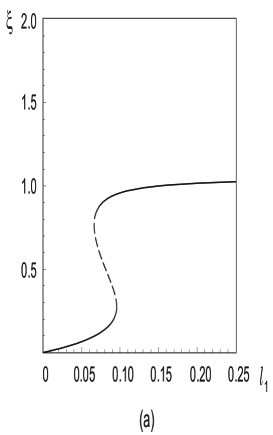
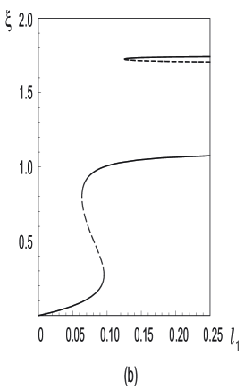
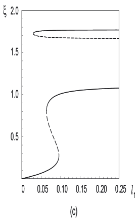
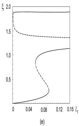
Figure 8: Equilibrium position of oscillator $\xi$ vs the concentration $\ell_{1}$ for different values of $S_{0}$: $S_{0}$ = 0.0003 (a), 0.000475 (b), 0.00048 (c), 0.00055 (d), 0.00064 (e), 0.00066 (f); $G=2,g_{1}=5$.

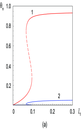
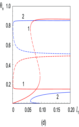
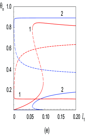
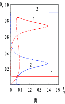
Figure 9: Surface coverages $\theta_{n}$ by adparticles of species $n$ ($n=1$, curve 1; $n=2$, curve 2) vs the concentration $\ell_{1}$. The values of $S_{0},G$, and $g_{1}$ are the same as in Fig. 8.

The graphs of the equilibrium position of oscillator $\xi(\ell_{1})$ and the surface coverages $\theta_{n}(\ell_{1})$ for $g_{1}=5$ depicted in Figs. 8 and 9, respectively, illustrate specific features of these functions in the case where a stationary solution of system (7) can have several asymptotes. In this case, $S^{a}_{-}\approx 0.0004734$ and $S^{a}_{+}\approx 0.0006462$.

For $S_{0}<S^{a}_{-}$, the coordinate $\xi(\ell_{1})$ (Fig. 8a) and the surface coverages $\theta_{n}(\ell_{1})$ (Fig. 9a) have a hysteresis typical of these quantities in adsorption of a one-component gas for values of the coupling parameter greater than critical [27] or a two-component gas, e.g., for $g_{1}\in(3,4)$ and $S_{0}\in(S^{c}_{-},\,S^{c}_{+})$ (see Figs. 6b and 7b). The coordinate $\xi(\ell_{1})$ consists of three branches: two stable branches (the lower stable branch for $\ell_{1}\in[0,\,\ell^{b}_{1,2}]$ and the upper stable branch for $\ell_{1}\in[\ell^{b}_{1,1},\,\infty)$ that approaches its horizontal asymptote $\xi=\xi^{a}_{1}$ as $\ell_{1}$ increases) and one unstable branch connecting them. The surface coverages $\theta_{n}(\ell_{1})$ have a similar shape. For all considered values of $S_{0}$, the lower stable branch of $\theta_{2}(\ell_{1})$ in Fig. 9 almost coincides with the abscissa axis.

For $S_{0}\in(S^{a}_{-},\,S^{a}_{+})$, the behavior of $\xi(\ell_{1})$ and $\theta_{n}(\ell_{1})$ qualitatively differs from their behavior in Figs. 6 and 7. For $S_{0}>S^{a}_{-}$, there appears an isolated piece of $\xi(\ell_{1})$ with semiinfinite domain of definition $\ell_{1}\in[\ell^{b}_{1,3},\,\infty)$ (Fig. 8b). This isolated piece consists of stable and unstable branches starting at the bifurcation concentration $\ell^{b}_{1,3}$ and rapidly tending to closely lying asymptotes $\xi=\xi^{a}_{3}$ and $\xi=\xi^{a}_{2}$ ($\xi^{a}_{3}>\xi^{a}_{2}$), respectively, as $\ell_{1}$ increases. Thus, the range of values of the positive-definite function $\xi(\ell_{1})$ consists of two intervals ($\xi\in[0,\,\xi^{a}_{1})$ and $\xi\in(\xi^{a}_{2},\,\xi^{a}_{3})$) with gap $\xi\in(\xi^{a}_{1},\,\xi^{a}_{2})$ between them. According to the principle of perfect delay [36, 37], the transition from the first piece ($\xi\in[0,\,\xi^{a}_{1})$) of $\xi(\ell_{1})$ to the isolated piece ($\xi\in(\xi^{a}_{2},\,\xi^{a}_{3})$) with variation in the concentration $\ell_{1}$ is impossible for any initial value of $\ell_{1}$. If the initial state of the system lies on the stable branch of the isolated piece of $\xi(\ell_{1})$, then, as $\ell_{1}$ decreases, the coordinate $\xi$ varies along this branch up to its end at $\ell_{1}=\ell^{b}_{1,3}$, then jumps down to the upper stable branch of the first piece of $\xi(\ell_{1})$ and varies along it in the same way as in Fig. 8a.

Since the behavior of the surface coverage $\theta_{2}(\ell_{1})$ in Fig. 9b is similar to the behavior of the coordinate $\xi(\ell_{1})$ in Fig. 8b, all conclusions for $\xi(\ell_{1})$ remain true for $\theta_{2}(\ell_{1})$. Moreover, this also holds for other values of $S_{0}$ (cf. curve 2 in Fig. 9c–f with curve in Fig. 8c–f).

The surface coverage $\theta_{1}(\ell_{1})$ in Fig. 9b also has the isolated piece. However, unlike the isolated pieces of the surface coverage $\theta_{2}(\ell_{1})$ and the coordinate $\xi(\ell_{1})$ (Fig. 8b), it lies below the asymptote $\theta_{1}=\theta^{a}_{1,1}$ of the first piece of $\theta_{1}(\ell_{1})$, $\ \theta^{a}_{1,1}>\theta^{a}_{1,2}>\theta^{a}_{1,3}$.

As $S_{0}\in(S^{a}_{-},\,S^{a}_{+})$ increases, the isolated piece of $\xi(\ell_{1})$ shifts to the ordinate axis (the bifurcation concentration $\ell^{b}_{1,3}$ decreases), its thickness increases, and, in a certain interval of $\ell_{1}$, the system is tristable (Fig. 8c–e). As above, the transition from the first piece of $\xi(\ell_{1})$ to the isolated piece with variation in $\ell_{1}$ is impossible. However, as the concentration $\ell_{1}$ decreases, the transition from the stable branch of the isolated piece of $\xi(\ell_{1})$ to the lower stable branch (rather than the upper stable branch as in Fig. 8b) of the first piece of $\xi(\ell_{1})$ occurs at $\ell_{1}=\ell^{b}_{1,3}$.

Unlike the surface coverage $\theta_{2}(\ell_{1})$, the pieces of the surface coverage $\theta_{1}(\ell_{1})$ in Figs. 9c–e intersect one another. However, the continuous transition between stable branches of the different pieces of $\theta_{1}(\ell_{1})$ at the point of their intersection is forbidden by the condition for transition between stationary solutions of the system.

For $S_{0}>S^{a}_{+}$, the gap between two pieces of $\xi(\ell_{1})$ disappears ($\ell^{b}_{1,4}$ is finite) and the function $\xi(\ell_{1})$ is continuous and has three stable and two unstable branches (Fig. 8f). There are two bistability intervals $(\ell^{b}_{1,3},\,\ell^{b}_{1,1})$ and $(\ell^{b}_{1,2},\,\ell^{b}_{1,4})$ and one tristability interval $(\ell^{b}_{1,1},\,\ell^{b}_{1,2})$ between them. The graph of the surface coverage $\theta_{1}(\ell_{1})$ in Fig. 9f is also continuous and consists of three stable branches and two unstable branches connecting them. However, the shapes of $\theta_{1}(\ell_{1})$ and $\theta_{2}(\ell_{1})$ are essentially different. For $\ell_{1}>\ell^{b}_{1,4}$, the adsorption sites are considerably displaced from their nonperturbed equilibrium position $\xi=0$ so that the coordinate $\xi(\ell_{1})$ is, in fact, a constant (Fig. 8f). In this case, an almost monolayer coverage of the surface mainly by adparticles of species 2 occurs (cf. the flat regions of the curves in Fig. 9f), whereas, in the classical case, the surface coverage by adparticles of species 2 is less than 0.1% of the total coverage.

4 Adiabatic Approximation

The specific features of stationary solutions of system (7) investigated in Sec. 3 can be explained with the use of a potential. To this end, we consider the last equation of system (7) in the overdamped approximation where the masses of an adsorption site and adparticles are low and the friction coefficient is so large that the first term on the left-hand side of this equation can be neglected as against the second. Using the well-known results for a linear free oscillator of constant mass [38], this approximation is correct if

$$\tau^{2}_{M}\ll\tau^{2}_{r},$$ (67)

where $\tau_{M}=1/\omega_{M}$, $\omega_{M}=\sqrt{\varkappa/M}$ is the vibration frequency of an oscillator of mass $M$, and $\tau_{r}=\alpha/\varkappa$ is the typical relaxation time of a massless oscillator.

Further, consider the case where the relaxation time of the coordinate $\xi(t)$ of a massless oscillator is much greater than the relaxation times of the surface coverages $\theta_{n}(t),\ n=1,2$, in the linear case, i.e., the variables $\xi$ and $\theta_{n}$ are slow and fast, respectively. In this case, $\tau_{r}\gg\tau_{\theta}$, where

$$\tau_{\theta}\approx 2\,\Biggl{\{}\biggl{(}\frac{1}{\tau^{ad}_{1}}+\frac{1}{\tau^{ad}_{2}}\biggr{)}-\sqrt{\biggl{(}\frac{1}{\tau^{ad}_{1}}-\frac{1}{\tau^{ad}_{2}}\biggr{)}^{2}+\frac{4}{\tau^{a}_{1}\,\tau^{a}_{2}}\ }\,\Biggr{\}}^{-1},$$ (68)

$\tau^{ad}_{n}=\tau^{a}_{n}\,\tau^{d}_{n}/(\tau^{a}_{n}+\tau^{d}_{n})$ is the time taken for attaining the stationary value of the surface coverage $\theta_{n}$ in the case of the Langmuir adsorption of a one-component gas particles of species $n$ and $\tau^{a}_{n}=1/k^{a}_{n}C_{n},\ n=1,2$, can be regarded as the typical lifetime of a vacant adsorption site in this case. Using the principle of adiabatic elimination of the fast variables $\theta_{n}(t)$ in (7) [39], we set $d\theta_{n}/dt=0,\ n=1,2$, and express the surface coverage $\theta_{1}$ vs the slow variable $\xi$ as follows:

$$\theta_{1}=\frac{\ell_{1}}{\ell_{1}\left(1+S(\xi)\right)+\exp(-g_{1}\,\xi)}\,.$$ (69)

The surface coverage $\theta_{2}$ is defined by relation (17) with $\theta_{1}$ given by relation (63). The coordinate $\xi(t)$ is determined as a solution of the nonlinear differential equation

$$\alpha\frac{d\xi}{dt}=-\frac{dU(\xi)}{d\xi}$$ (70)

that describes the motion of a massless oscillator in the potential

$$U(\xi)=\frac{\varkappa}{2}\,\biggl{\{}\xi^{2}-2\,h(\xi)\biggr{\}},$$ (71)

where the second term on the right-hand of (65) caused by the adsorption-induced force acting on an adsorption site has the form

$$h(\xi)=\ell_{1}\int\limits_{0}^{\xi}\!\!dy\,\frac{1+G\,S(y)}{\ell_{1}\left(1+S(y)\right)+\exp(-g_{1}\,y)}\,.$$ (72)

Relations (17), (63), and (64) correctly describe the behavior of the dynamical variables $\xi(t)$ and $\theta_{n}(t)$ for times $t\gg\tau_{\theta}$ for which the fast variables $\theta_{n}(t)$ forget the initial data.

The shape of $U(\xi)$ essentially depends on the control parameters $\ell_{1},g_{1},S_{0}$, and $G$. The stationary solutions $\xi_{j}$ of Eq. (64), where the subscript $j$ is the number of a stationary solution, are roots of Eq. (18) and, furthermore, the number of roots vary from 1 to 5 depending on the values of the control parameters. Roots are enumerated so that $\xi_{j+1}>\xi_{j}$, and $U_{j}\equiv U(\xi_{j})$. In the case of simple roots, odd and even values of $j$ correspond to stable (minima of $U(\xi)$) and unstable (maxima of $U(\xi)$) stationary solutions of Eq. (64), respectively. For a double root $\xi_{j}$, the potential has a horizontal point of inflection at $\xi=\xi_{j}$ and Eq. (64) has a two-fold stationary solution.

In the special case of the identical action of adparticles on the adsorbent ($G=1$), relation (65) is reduced to the potential in adsorption of a one-component gas on a deformable adsorbent [27] with $\ell$ replaced by $\ell_{+}$

$$U(\xi)=\frac{\varkappa}{2}\,\biggl{\{}\xi^{2}-2\,\xi-\frac{2}{g}\,\ln{\frac{\ell_{+}+\exp{\left(-g\,\xi\,\right)}}{\ell_{+}+1}}\biggr{\}}.$$ (73)

Using results for one-component adsorption [27], we conclude that, for $g>4$ and $\ell_{+}\in(\ell^{b}_{+,1},\,\ell^{b}_{+,2})$, $U(\xi)$ is a two-well potential with local minima at $\xi=\xi_{1}$ and $\xi=\xi_{3}$ separated by a maximum at $\xi=\xi_{2}$, where $\xi_{j},\ j=1,2,3$, are the coordinates determined from Eq. (36) with regard for relation (35). Thus, in this case, the system under study is bistable. For $g<4$ and any concentrations $\ell_{1}$ and $\ell_{2}$ as well as for $g>4$ and $\ell_{+}\notin[\ell^{b}_{+,1},\,\ell^{b}_{+,2}]$, the potential $U(\xi)$ has one minimum and, hence, the considered system is monostable.

In another special case where adparticles of species 2 do not affect the adsorbent deformation ($G=0$), the potential is also defined by relation (67) with $\ell_{+}$ replaced by $\ell_{1}/(1+\ell_{2})$.

In what follows, we analyze the potential $U(\xi)$ in the case $G=2$ for which the coordinate $\xi(\ell_{1})$ and the surface coverages $\theta_{n}(\ell_{1})$ have been investigated in Secs. 3.4, 3.5.

For $g_{1}\in(3,4)$, $U(\xi)$ is a single-well potential if $S_{0}<S^{c}_{-}$. For the given values of the parameters $g_{1}$ and $S_{0}$, the depth of the well $|U_{1}|$ and the position of its minimum $\xi_{1}$ increase with $\ell_{1}$. As $S_{0}$ increases, for $S_{0}>S^{c}_{-}$, the situation cardinally changes and, for the given value of $g_{1}$, the shape of the potential essentially depends on the values of $\ell_{1}$ and $S_{0}$. If $S_{0}\in(S^{c}_{-},\,S^{c}_{+})$, then the potential has either two minima if $\ell_{1}\in(\ell^{b}_{1,1},\,\ell^{b}_{1,2})$ or one minimum if $\ell_{1}\notin[\ell^{b}_{1,1},\,\ell^{b}_{1,2}]$.

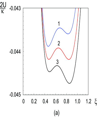
Figure 10: Normalized potential for $G=2$, $g_{1}=3.5$, $S_{0}$ = 0.0055, and different values of the concentration $\ell_{1}$: $\ell_{1}=$ 0.158 (1), 0.15826 (2), 0.1585 (3) (a); $\ell^{b}_{1,1}$ (1), 0.1582 (2), $\ell^{b}_{1,2}$ (3) (b).

For $S_{0}=0.0055\in(S^{c}_{-},\,S^{c}_{+})$, the curves in Fig. 10a illustrate the two-well shape of the potential for $\ell_{1}\in(\ell^{b}_{1,1},\,\ell^{b}_{1,2})$, where $\ell^{b}_{1,1}\approx 0.1575$ and $\ell^{b}_{1,2}\approx 0.159$. The curves in Fig. 10b show essential changes in the shape of the potential for the bifurcation concentrations $\ell^{b}_{1,1}$ (curve 1) and $\ell^{b}_{1,2}$ (curve 3), namely, as $\ell_{1}$ increases, the single-well potential for $\ell_{1}<\ell^{b}_{1,1}$ is transformed into a two-well one for $\ell_{1}>\ell^{b}_{1,1}$ and then the two-well potential for $\ell_{1}\in(\ell^{b}_{1,1},\,\ell^{b}_{1,2})$ is transformed into a single-well one for $\ell_{1}>\ell^{b}_{1,2}$. Curve 1 in Fig. 10a shows the appearance of the second stationary (metastable because $U_{1}<U_{3}$) state of the system at the greater displacement $\xi_{3}$ ($\xi_{3}>\xi_{1}$) of the oscillator from its nonperturbed equilibrium position $\xi=0$. An increase in $\ell_{1}$ is accompanied by an increase in the depths of both wells and a decrease in the barrier $\delta_{2,1}=U_{2}-U_{1}$ between the wells. Since the increment of the depth of the second well with $\ell_{1}$ is greater than that of the first well, for a certain value of $\ell_{1}$, the depths of the wells become approximately equal (curve 2 in Fig. 10a) and, for greater values of $\ell_{1}$, the second well is deeper than the first (curve 3 in Fig. 10a), i.e., the state of the system becomes metastable in the first well and stable in the second. Nevertheless, within the framework of the overdamped approximation, following the principle of perfect delay [36, 37], as $\ell_{1}$ increases, the oscillator remains in the first well rather than moves to the second. For transition of the system from the metastable state to the stable state according to the Maxwell principle of the choice of the global minimum of the potential [36, 37], thermal fluctuations or the inertia effect (as in [40] in the case of one-component adsorption) or both these factors should be taken into account. This situation remains up to the bifurcation concentration $\ell^{b}_{1,2}$ for which the barrier $\delta_{2,1}=0$ (curve 3 in Fig. 10b). A negligible excess of this bifurcation concentration leads to the transformation of the potential into a single-well potential, which is accompanied by the displacement of the oscillator to the unique equilibrium position at the point $\xi_{3}$ or, in terms of $\xi(\ell_{1})$, the transition of the coordinate $\xi(\ell_{1})$ from its lower stable branch to the upper one at $\ell_{1}=\ell^{b}_{1,2}$ (see Fig. 6b). In turn, this is accompanied by transitions of the surface coverages $\theta_{n}(\ell_{1})$ from their lower stable branches to the upper ones (Fig. 7b).

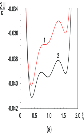
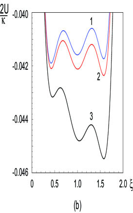
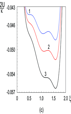
Figure 11: Normalized potential for $G=2$, $g_{1}=3.5$, $S_{0}$ = 0.00585, and different values of the concentration $\ell_{1}$: $\ell_{1}=$ $\ell^{b}_{1,1}$ (1), 0.155 (2) (a); 0.1558 (1), 0.156 (2), 0.157 (3) (b); $\ell^{b}_{1,2}$ (1), 0.159 (2), $\ell^{b}_{1,4}$ (3) (c).

The curves in Fig. 11 for $S_{0}=0.00585\in(S^{c}_{d},\,S^{c}_{t})$ illustrate the transformation of the two-well potential $U(\xi)$ for $\ell_{1}<\ell^{b}_{1,1}\approx 0.154$ into a three-well one and vice versa for $\ell_{1}>\ell^{b}_{1,2}\approx 0.158$ as $\ell_{1}$ increases. For the bifurcation concentration $\ell^{b}_{1,1}$, the potential has two wells and the horizontal point of inflection between them (curve 1 in Fig. 11a). As the concentration $\ell_{1}$ increases, the potential is deformed in the neighborhood of this point of inflection so that there appears one more well (curve 2 in Fig. 11a), which corresponds to the case of five simple roots of Eq. (18). The depths of the wells at $\xi=\xi_{j}$, where $j=1,3,5$, decrease with $\xi$: $|U_{1}|>|U_{3}|>|U_{5}|$. As $\ell_{1}$ increases, this inequality is replaced, first, by $|U_{1}|>|U_{5}|>|U_{3}|$ (curve 1 in Fig. 11b) and then by $|U_{5}|>|U_{3}|>|U_{1}|$ (curves 2 and 3 in Fig. 11b), i.e., the deepest well successively moves away from the nonperturbed equilibrium position $\xi=0$ with $\ell_{1}$. For the bifurcation concentration $\ell^{b}_{1,2}$ the barrier between the first and second wells disappears, $\delta_{2,1}=0$ (curve 1 in Fig. 11c). A negligible excess of this bifurcation concentration leads to the transformation of $U(\xi)$ into a two-well potential and, as a result, the displacement of the oscillator to the equilibrium position at the point $\xi_{3}$ or, in terms of $\xi(\ell_{1})$, the transition of the coordinate $\xi(\ell_{1})$ from its first stable branch to the second at $\ell_{1}=\ell^{b}_{1,2}$ (Fig. 6f). In turn, this is accompanied by transitions of the surface coverages $\theta_{n}(\ell_{1})$ from their first stable branches to the second (Fig. 7f). As $\ell_{1}$ increases, the two-well potential is transformed so that the barrier between two remaining wells $\delta_{4,3}=U_{4}-U_{3}$ decreases and becomes equal to zero for the bifurcation concentration $\ell^{b}_{1,4}\approx 0.161$ (curve 3 in Fig. 11c). For $\ell_{1}>\ell^{b}_{1,4}$, only one well of the potential $U(\xi)$ most remote from the nonperturbed surface remains and the oscillator shifts to the bottom of this well at $\xi=\xi_{5}$.

Taking into account the different increase in the residence times of adparticles of different species on the surface with displacement of adsorption sites from the nonperturbed adsorbent surface [see (9)–(14)], we can draw a conclusion on a considerable increase in the fraction of adparticles of species 2 in the total amount of adsorbed substance in transition of adsorption sites to a more remote well. This conclusion explains, in particular, the opposite behavior of the surfaces coverages $\theta_{1}(\ell_{1})$ and $\theta_{2}(\ell_{1})$ in Figs. 7c–f, 7i in passing through the bifurcation value $\ell^{b}_{1,4}$: a stepwise decrease in $\theta_{1}(\ell_{1})$ and a stepwise increase in $\theta_{2}(\ell_{1})$ are caused by the displacement of the adsorption sites to the most remote well.

As has been shown in Sec. 3.1, the specific feature of adsorption of a two-component gas on a deformable adsorbent is two stable horizontal asymptotes of the coordinate $\xi(\ell_{1})$ and the surface coverages $\theta_{n}(\ell_{1})$ for certain values of control parameters. To explain this effect in terms of the potential $U(\xi)$, we investigate its behavior in the limiting case of infinitely large values of $\ell_{1}$. Passing in (66) to the limit $\ell_{1}\rightarrow\infty$, we obtain

$$U^{a}(\xi)\equiv\lim\limits_{\ell_{1}\rightarrow\infty}U(\xi)=\frac{\varkappa}{2}\,\biggl{\{}\xi^{2}-2\,\xi-\frac{2}{g_{1}}\ln{\frac{1+S(\xi)}{1+S_{0}}}\biggr{\}}.$$ (74)

For a finite concentration of gas particles of species 2 (in the special case of one-component adsorption, $\ell_{2}=0$), relation (68) is reduced to the parabolic potential

$$U^{a}(\xi)=\varkappa\,\xi\biggl{(}\frac{\xi}{2}-1\biggr{)}$$ (75)

with minimum at the point $\xi=1$, which, according to (24), gives the unique horizontal asymptotes $\theta^{a}_{1}=1$ and $\theta^{a}_{2}=0$ for the surface coverages $\theta_{1}(\ell_{1})$ and $\theta_{2}(\ell_{1})$, respectively.

In the special case of adsorption of a two-component gas with identical action of adparticles on the adsorbent ($G=1$), relation (69) remains also true for $\ell_{2}=\infty$.

Taking into account that the functions $\xi(\ell_{1})$ and $\theta_{n}(\ell_{1})$ have two stable horizontal asymptotes if $g_{1}>g^{a}_{c}$ and, e.g., $S_{0}\in(S^{a}_{-},S^{a}_{+})$ for $G>1$, we conclude that, for these values of the parameters $G$, $g_{1}$, and $S_{0}$, $U^{a}(\xi)$ is a two-well potential and the system under study is bistable in a semiinfinite interval of values of $\ell_{1}$.

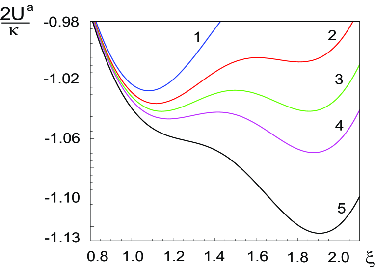
Figure 12: Normalized potential for $\ell_{1}=\infty$, $G=2$, $g_{1}=5$, and different values of $S_{0}$: $S_{0}$ = 0.0004 (1), 0.0005 (2), 0.000553 (3), 0.0006 (4), 0.0007 (5).

The curves in Fig. 12 clearly illustrate the essential dependence of the potential $U^{a}(\xi)$ on the value of $S_{0}$. For $S_{0}<S^{a}_{-}\approx 0.000473$ (curve 1) and $S_{0}>S^{a}_{+}\approx 0.000646$ (curve 5), the potential has one well; furthermore, in the second case, the well is deeper and considerably more shifted from the nonperturbed adsorbent surface $\xi=0$. For $S_{0}\in(S^{a}_{-},S^{a}_{+})$, the potential has two wells; moreover, if $S_{0}$ is close to $S^{a}_{-}$, then the first well is deeper than the second (curve 2) and if $S_{0}$ is close to $S^{a}_{+}$, then the second well is deeper than the first (curve 4). Curve 3 corresponds to the case of approximately equal depths of the wells. The two-well potential $U^{a}(\xi)$ leads to two disconnected pieces of the coordinate $\xi(\ell_{1})$ (see Fig. 8b–e) and the corresponding specific features of the surface coverages $\theta_{1}(\ell_{1})$ and $\theta_{2}(\ell_{1})$ (see Fig. 9b–e).

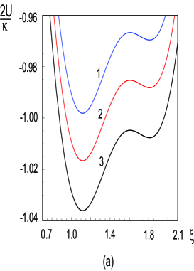
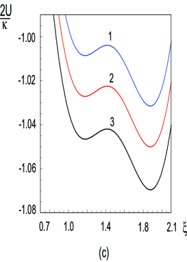
Figure 13: Normalized potential for $G=2$, $g_{1}=5$, the concentration $\ell_{1}=$ 10 (1), 20 (2), $\infty$ (3), and $S_{0}$ = 0.0005 (a), 0.000553 (b), 0.0006 (c).

The curves in Fig. 13 illustrate the approach of the potential $U(\xi)$ to the two-well potential $U^{a}(\xi)$ as the concentration $\ell_{1}$ increases. For large values of $\ell_{1}$, the behavior of the two-well potential $U(\xi)$ is similar to $U^{a}(\xi)$: the first well is deeper if $S_{0}$ is close to $S^{a}_{-}$ (Fig. 13a), the second well is deeper if $S_{0}$ is close to $S^{a}_{+}$ (Fig. 13c), the depths of two wells in figure 11(b) are approximately equal. Note that, according to the principle of perfect delay [36, 37], the oscillator remains in the first well for arbitrarily large values of $\ell_{1}$.

5 Conclusions

In the present paper, we have investigated isotherms of competitive adsorption of a two-component gas on the surface of a solid adsorbent whose adsorption properties vary in adsorption due to the adsorbent deformation. It has been established that taking account of the adsorbent deformation in adsorption essentially changes the shape of adsorption isotherms relative to the Langmuir isotherms. The specific features of adsorption isotherms (bistability and tristability of the system, two stable asymptotes of adsorption isotherms, an essential redistribution of the quantities of adsorbed particles of different species as compared with those in the classical case) depend on values of the parameters expressed in terms of the phenomenological constant adsorption-induced forces $\chi_{1}$ and $\chi_{2}$. The values of these forces can be determined knowing experimental data of changes in the first interplanar spacing (along the normal to the surface) $x_{n}^{max}$ due to the total monolayer coverage of the adsorbent surface by adparticles of species $n$ in adsorption of a one-component gas. In terms of the measured $x_{n}^{max}$, the required forces and the coupling parameters are expressed as follows:

$$\chi_{n}=\varkappa\,x_{n}^{max},\qquad g_{n}=\varkappa\,(x_{n}^{max})^{2}/k_{B}T,\quad n=1,2,\qquad G=x_{2}^{max}/x_{1}^{max}.$$ (76)

Based on the values of the parameters calculated by relations (70), one can conclude whether the specific features of adsorption isotherms of a binary gas mixture established in the paper are possible or not. According to (70), this is more probable for adsorbents with relatively low elastic characteristics and a surface layer susceptible to a change in the spatial distribution of the charge density of adsorption sites in adsorption and resulting in not too low absolute values of adsorption-induced forces. Possibly, in experiments aimed at searching for these effects caused by the adsorbent deformation in adsorption, it makes sense to use single crystal solid substrates of a “soft” material admitting a considerable normal displacement of the adsorbent surface in adsorption.

It is also worth noting that the used mean-field approximation requires that the relaxation time of a bound adsorption site to a new equilibrium position caused by adsorption be much greater than the average time between collisions of gas particles with the adsorption site and the average residence time of an adparticle on the surface. For this relaxation time to be much more greater than the vibrational period of a vacant adsorption site, the friction coefficient must be not negligible. This leads to a certain condition imposed on its value, which depends on the concentration of particles in the gas phase, so that many gas particles can successively take part in adsorption on the same adsorption site before it reaches the equilibrium position.

The proposed model of competitive adsorption of a two-component gas on a deformable adsorbent should be regarded as only the first step for describing adsorption on a deformable adsorbent. The subsequent development of the model requires taking account of various factors (lateral interactions between adparticles, fluctuations, energy inhomogeneity of the adsorbent surface, etc.) not considered here.

References

- [1] S. R. Morrison, The Chemical Physics of Surfaces (Plenum, New York, 1977).
- [2] M. W. Roberts and C. S. McKee, Chemistry of the Metal–Gas Interface (Oxford University Press, Oxford, 1978).
- [3] A. G. Naumovets, Studies of surface structure by the low-energy electron diffraction method: achievements and outlooks, Ukr. Fiz. Zh., 23, No. 10, 1585–1607 (1978).
- [4] M. J. Jaycock and G. D. Parfitt, Chemistry of Interfaces (Wiley, New York, 1981).
- [5] V. F. Kiselev and O. V. Krylov, Adsorption Processes on Semiconductor and Dielectric Surfaces (Springer, Berlin, 1985).
- [6] F. F. Vol’kenshtein, Electron Properties on Semiconductor Surfaces at Chemisorption (Nauka, Moscow, 1987).
- [7] A. Zangwill, Physics at Surfaces (Cambridge University Press, Cambridge, 1988).
- [8] V. D. Zhdanov, Elementary Physicochemical Processes on Solid Surfaces (Plenum, New York, 1991).
- [9] I. F. Lyuksyutov, A. G. Naumovets, and V. L. Pokrovsky, Two-Dimensional Crystals (Academic, Boston, 1992).
- [10] A. W. Adamson and A. P. Cast, Physical Chemistry of Surfaces (Wiley, New York, 1997).
- [11] A. G. Naumovets, Use of surface phase transitions for control over properties of surfaces, in: I. K. Pohodnya, A. H. Kostornov, Yu. M. Koval’, et al., Progressive Materials and Technologies, Vol. 2 (Akademperiodyka, Kyiv, 2003), pp. 319–350.
- [12] P. Barret, Cinétique Hétérogène (Guathier-Villars, Paris, 1973).
- [13] S. Z. Roginskii, Heterogeneous Catalysis. Some Problems of the Theory (Nauka, Moscow, 1979).
- [14] A. Ya. Rozovskii, Heterogeneous Chemical Reactions. Kinetics and Macrokinetics (Nauka, Moscow, 1980).
- [15] G. K. Boreskov, Heterogeneous Catalysis (Nauka, Moscow, 1986).
- [16] O. V. Krylov and B. R. Shub, Nonequilibrium Processes in Catalysis (CRC Press, Boca Raton, 1994).
- [17] O. V. Krylov, Heterogeneous Catalysis (Akademkniga, Moscow, 2004).
- [18] D. A. Frank-Kamenetskii, Diffusion and Heat Transfer in Chemical Kinetics (Plenum, New York, 1969).
- [19] D. M. Ruthven, Principles of Adsorption and Adsorption Processes (Willey, Chichester, 1984).
- [20] Yu. L. Tovbin, Theory of Physical Chemistry Processes at a Gas–Solid Interface (CRC Press, Boca Raton, 1991).
- [21] D. D. Do, Adsorption Analysis: Equilibria and Kinetics (Imperial College Press, London 1998).
- [22] J. Keller and R. Staudt, Gas Adsorption Equilibria: Experimental Methods and Adsorption Isotherms (Springer, 2005).
- [23] R. Imbihl and G. Ertl, Oscillatory kinetics in heterogeneous catalysis, Chem. Rev., 95, No. 3, 697–733 (1995).
- [24] R. Imbihl, Nonlinear dynamics on catalytic surfaces, Catal. Today, 105, 206–222 (2005).
- [25] R. Imbihl, Nonlinear dynamics on catalytic surfaces: The contribution of surface science, Surf. Sci., 603, 1671–1679 (2009).
- [26] G. Ertl, Reactions at Solid Surfaces (Wiley, Hoboken, 2009).
- [27] A. S. Usenko, Adsorption on a surface with varying properties, Phys. Scr., 85, 015601 (2012).
- [28] Ya. B. Zeldovich, Adsorption on a uniform surface, Acta Physicochim. URSS, 8, No. 5, 527–530 (1938).
- [29] T. Ala-Nissila, R. Ferrando, and S. G. Ying, Collective and single particle diffusion on surfaces, Adv. Phys., 51, No. 3, 949–1078 (2002).
- [30] Z.-J. Tan, X.-W. Zou, S.-Y. Huang, W. Zhang, and Z.-Z. Jin, Patterns of particle distribution in multiparticle systems by random walks with memory enhancement and decay, Phys. Rev. B, 66, 011101 (2002).
- [31] S.-Y. Huang, X.-W. Zou, and Z.-Z. Jin, Multiparticle random walks on a deformable medium, Phys. Rev. B, 66, 041112 (2002).
- [32] R. T. Yang, Adsorbents: Foundations and Applications (Wiley, Hoboken, 2003).
- [33] V. M. Gun’ko, Competitive adsorption, Theor. Experim. Chem., 43, No. 3, 133–182 (2007).
- [34] A. G. Naumovets, Adsorption on metals: a look from the not-too-far East, Surf. Sci., 299/300, 706–721 (1994).
- [35] L. N. Christophorov, A. R. Holzwarth, V. N. Kharkyanen, and F. van Mourik, Structure-function self-organization in nonequilibrium macromolecular systems, Chem. Phys., 256, 45–60 (2000).
- [36] T. Poston and I. Stewart, Catastrophe Theory and Its Applications (Pitman, London 1978).
- [37] R. Gilmore, Catastrophe Theory for Scientists and Engineers (Wiley, New York, 1981).
- [38] A. A. Andronov, A. A. Vitt, and S. É. Khaikin, Theory of Oscillators (Pergamon, New York, 1966).
- [39] H. Haken, Synergetics (Springer, Berlin, 1978).
- [40] A. S. Usenko, Adsorption on a Surface with Varying Properties, arXiv: 0907.5569v2 (2009).