Scalable Anomaly Detection in Large Homogenous Populations

Abstract

Anomaly detection in large populations is a challenging but highly relevant problem. The problem is essentially a multi-hypothesis problem, with a hypothesis for every division of the systems into normal and anomal systems. The number of hypothesis grows rapidly with the number of systems and approximate solutions become a necessity for any problems of practical interests. In the current paper we take an optimization approach to this multi-hypothesis problem. We first observe that the problem is equivalent to a non-convex combinatorial optimization problem. We then relax the problem to a convex problem that can be solved distributively on the systems and that stays computationally tractable as the number of systems increase. An interesting property of the proposed method is that it can under certain conditions be shown to give exactly the same result as the combinatorial multi-hypothesis problem and the relaxation is hence tight.

, , , ,

1 Introduction

In this paper we study the following problem: We are given $N$ systems and we suspect that $k\ll N$ of them behave differently from the majority. We do not know beforehand what the normal behavior is, and we do not know which $k$ systems that behave differently. This problem is known as an anomaly detection problem and has been discussed e.g., in [9, 11, 17]. It clearly has links to change detection (e.g., [23, 4, 18]) but is different because the detection of anomalies is done by comparing systems rather than looking for changes over time.

The anomaly detection problem typically becomes very computationally demanding, and it is therefore of interest to study distributed solutions. A distributed solution is also motivated by that many anomaly detection problems are spatially distributed and lack a central computational unit.

Example 1 (Aircraft Anomaly Detection).

In this example we consider the problem of detecting abnormally behaving airplanes in a large homogenous fleet of aircrafts. Homogenous here means that the normal aircrafts have similar dynamics. This is a very relevant problem [11, 17] and of highest interest for safety in aeronautics. In fact, airplanes are constantly gathering data and being monitored for this exact reason. In particular, so called flight operations quality assurance (FOQA) data are collected by several airlines and used to improve their fleet’s safety.

As showed in [11], faults in the angle-of-attack channel can be detected by studying the relation between the angle of attack, the dynamic pressure, mass variation, the stabilizer deflection angle, and the elevator deflection. The number of airplanes in a fleet might be of the order of hundreds and data from a couple of thousand flights might be available (200 airplanes and data from 5000 flights were used in [11]). Say that our goal is to find the 3 airplanes among 200 airplanes that are the most likely to be anomal to narrow the airplanes that need manual inspection. Then, we would have to evaluate roughly $1.3\times 10^{6}$ hypothesis (the number of unordered selections of 3 out of 200 airplanes). For each hypothesis, the likelihood for the observed data would then be maximized with respect to the unknown parameters and the most likely hypothesis accepted. This is clearly a very computationally challenging problem.

Example 1 considers anomaly detection in a large homogenous population and is the type of problem we are interested in solving in this paper. The problem has previously been approached using model based anomaly detection methods, see e.g., [11, 17, 9]. This class of anomaly detection methods is suitable to detect anomalies in systems, as opposed to non-model based methods that are more suitable for finding anomalies in data. Model based anomaly detection methods work under the assumption that the dynamics of normal systems are the same, or equivalently, that the population of systems is homogenous. The normal dynamics is modeled from system observations and most papers assume that an abnormal-free training data set is available for the estimation, see for instance [2, 1, 16]. Some papers have been presented to relax this assumption. In e.g., [24], the use of a regression technique robust to anomalies was suggested.

The detection of anomal systems is in model based anomaly detection done by comparing system observations and model predictions and often done by a statistical test, see e.g., [15, 12]. However, in non-model based anomaly detection, classification based [25, 14], clustering based [20], nearest neighbor based [25, Ch. 2], information theoretic [3] and spectral methods [22] are also common. See [9] for a detailed review of anomaly detection methods. Most interesting and similar to the proposed method is the more recent approach taken in [11, 17]. They simultaneously estimate the regression model for the normal dynamics and perform anomaly detection. The method of [11] is discussed further in the numerical section. There has also been some work on distributed anomaly detection, e.g., [28, 10, 11].

The main contribution of the paper is a novel distributed, scalable and model based method for anomaly detection in large homogenous populations. The method is distributed in the sense that the computations can be distributed over the systems in the population or a cluster of computers. It is scalable since the size of the optimization problem solved on each system is independent of the number of systems in the population. This is made possible by a novel formulation of the multi-hypothesis problem as a sparse problem. The method also shows superior performance and is easier to tune than previously proposed model based anomaly detection methods. Last, the method does not need a training data set and a regression model of the normal dynamics is estimated at the same time as abnormal systems are detected. This is particularly valuable since often neither a training data set or a regression model for the normal dynamics are available.

The remaining of the paper is organized as follows. Section 2 states the problem and shows the relation between anomaly detection and multi-hypothesis testing. Section 3 reformulates the multi-hypothesis problem as a sparse optimization problem and Section 4 gives a convex formulation. The convex problem is solved in a distributed manner on the systems and this is discussed in Section 5. We return to Example 1 and compare to the method of [11] in Section 6. Finally, we conclude the paper in Section 7.

2 Problem Statement and Formulation

Assume that the population of interest consists of $N$ systems. Think for example of the $N$ airplanes studied in Example 1. Further assume that there is a linear unknown relation describing the relation between measurable quantities of interest (angle of attack, the dynamic pressure, mass variation, the stabilizer deflection angle, and the elevator deflection in Example 1):

$$y_{i}(t)=\varphi_{i}^{\mathsf{T}}(t)\theta_{i,0}+e_{i}(t),\qquad i=1,\cdots,N,$$ (1)

where $t$ is the time index, $i$ indexing systems, $y_{i}(t)\in\mathbb{R}$ and $\varphi_{i}(t)\in\mathbb{R}^{m}$ are the measurement and regressor vector at time $t$, respectively, $\theta_{i,0}$ is the unknown model parameter, and $e_{i}(t)\in\mathbb{R}$ is the measurement noise. For the $i$th system, $i=1,\cdots,N$, let $\{(y_{i}(t),\varphi_{i}(t))\}_{t=1}^{\operatorname*{\Omega}}$ denote the collected data set and $\operatorname*{\Omega}$ the number of observations collected on each system. We assume that $e_{i}(t)$ is white Gaussian distributed with mean zero and some unknown variance $\sigma^{2}$ and moreover, independent of $e_{j}(t)$ for all $i\neq j$. However, log-concave distributed noise could be handled with minor changes.

We will in the following say that the population behaves normally and that none of the systems are abnormal if $\theta_{1,0}=\cdots=\theta_{N,0}=\theta_{0}$. Reversely, if any system has a model parameter deviating from the nominal parameter value $\theta_{0}$, we will consider that system as abnormal.

To solve the problem we could argue like this: Suppose we have a hypothesis about which $k$ systems are the anomalies. Then we could estimate the nominal parameters $\theta_{0}$ by least squares from the rest, and estimate individual $\theta_{i}$ for the $k$ anomalies. Since we do not know which systems are the anomalies we have to do this for all possible selections of $k$ systems from a set of $N$. This gives a total of

$$c(N,k)={N!}/\big{(}{(N-r)!r!}\big{)}$$ (2)

possible hypotheses. To decide which is the most likely hypothesis, we would evaluate the total misfit for all the systems, and choose that combination that gives the smallest total misfit. If we let $\gamma_{j}$ be the set of assumed abnormal systems associated with the $j$th hypothesis $j=1,\cdots,c(N,k)$, this would be equivalent to solving the the non-convex optimization problem

$$\operatorname*{minimize}_{j=1,\dots,c(N,k)} \sum_{s\in\gamma_{j}}\min_{\theta_{j,s}}\sum_{t=1,\cdots,\operatorname*{\Omega}}\|y_{s}(t)-\varphi_{s}^{\mathsf{T}}(t)\theta_{j,s}\|^{2}$$

$$+ \min_{\theta_{j,0}}\sum_{s\notin\gamma_{j},t=1,\cdots,\operatorname*{\Omega}}\|y_{s}(t)-\varphi_{s}^{\mathsf{T}}(t)\theta_{j,0}\|^{2}.$$ (3)

Since we assume that all systems have the same noise variance $\sigma^{2}$, this is a formal hypothesis test. If the systems may have different noise levels we would have to estimate these and include proper weighting in (3).

The difficulty is how to solve  (3) when the number of systems $N$ is large. As seen in Example 1, even for rather small examples ($k=3,\,N=200$), the number of hypothesis $c(N,k)$ becomes large and the problem (3) computationally intractable.

3 Sparse Optimization Formulation

A key observation to be able to solve the anomaly detection problem in a computationally efficient manner is the reformulation of the muti-hypothesis problem (3) as a sparse optimization problem. To do this, first notice that the multi-hypothesis test (3) will find the $k$ systems whose data are most likely to not have been generated from the same model as the remaining $N-k$ systems. Let us say that $j^{*}$ was the selected hypothesis and denote the parameter of the $i$th system by $\theta_{i}$, $i=1,\cdots,N$. Then $\theta_{i_{1}}\neq\theta_{i_{2}}$ for all $i_{1},i_{2}\in\gamma_{j^{*}}$ and $\theta_{i_{1}}=\theta_{i_{2}}$ for all $i_{1},i_{2}\in\{1,\cdots,N\}/\gamma_{j^{*}}$. Note that $N-k$ systems will have identical parameters. An equivalent way of solving the multi-hypothesis problem is therefore to maximize the likelihood under the constraint that $N-k$ systems are identical. This can be formulated as

$$\operatorname*{minimize}_{\theta_{1},\cdots,\theta_{N},\theta}\hskip 5.69054pt\sum_{i=1}^{N}\sum_{t=1}^{\operatorname*{\Omega}}\|y_{i}(t)-\varphi_{i}^{\mathsf{T}}(t)\theta_{i}\|^{2}$$ (4)

$$s.t.\hskip 2.84526pt\bigg{\|}\begin{bmatrix}\|\theta_{1}-\theta\|_{p}&\|\theta_{2}-\theta\|_{p}&\cdots&\|\theta_{N}-\theta\|_{p}\end{bmatrix}\bigg{\|}_{0}=k,$$

where $\theta$ denotes the nominal parameter, $\|\cdot\|_{0}$ is the zero-norm (pseudo norm) which counts the number of non-zero elements of its argument. In this way, the $k$ systems most likely to be abnormal could now be identified as the ones for which the estimated $\|\theta_{i}-\theta\|_{p}\neq 0$. Note that this is exactly the same problem as (3) and the same hypothesis will be selected.

Since abnormal model parameters and the nominal model parameter $\theta_{0}$ are estimated from the given data sets $\{(y_{i}(t),\varphi_{i}(t))\}_{t=1}^{\operatorname*{\Omega}}$, $i=1,\cdots,N$, that are subject to the measurement noise $e_{i}(t)$, $i=1,\cdots,N$, they are random variables. Moreover, it is well-known from [21, p. 282] that if the given data sets $\{(y_{i}(t),\varphi_{i}(t))\}_{t=1}^{\operatorname*{\Omega}}$, $i=1,\cdots,N$, are informative enough [21, Def. 8.1], then for each $i=1,\cdots,N$, the estimate of $\theta_{i}$ converges (as $\operatorname*{\Omega}\rightarrow\infty$) in distribution to the normal distribution with mean $\theta_{i,0}$ and covariance $M_{i}/\operatorname*{\Omega}$ where $M_{i}$ is a constant matrix which depends on $\theta_{i,0}$ and the data batch $\{(y_{i}(t),\varphi_{i}(t))\}_{t=1}^{\operatorname*{\Omega}}$. This implies that as $\operatorname*{\Omega}\rightarrow\infty$, (4) will solve the anomaly detection problem exactly, i.e., if there are $\tilde{k}\leq k$ systems that have a different model than the rest, those would be part of the hypothesis selected.

In the case where $\operatorname*{\Omega}$ is finite, our capability of correctly detecting the anomaly working systems will be dependent on the scale of the given $\operatorname*{\Omega}$ and $\sigma$, even with informative enough data sets $\{(y_{i}(t),\varphi_{i}(t))\}_{t=1}^{\operatorname*{\Omega}}$, $i=1,\cdots,N$. This is due to the fact that the variance of the estimate of $\theta_{i}$, $i=1,\cdots,N$, decreases as $\operatorname*{\Omega}$ and $1/\sigma$ increase. As a result, larger $\operatorname*{\Omega}$ and smaller $\sigma$ allow us to detect smaller model parameter deviations and hence increase our ability to detect abnormal behaviors.

Remark 3.1.

It should also be noted that if there is no overlap between observed features, anomalies can not be detected even in the noise free case. That is, if we let $Q$ be a $m\times m$-matrix with all zeros except for element $(q,q)$, which equals $1$, then if

$$\varphi^{\mathsf{T}}_{i}(t_{1})Q\varphi_{j}(t_{2})=0,\;j=1,\cdots,i-1,i+1,\cdots,N,\,\forall t_{1},t_{2},$$

a deviation in element $q$ in $\theta_{i}$ is not detectable. It can be shown that this corresponds to that the data is not informative enough.

4 Convex Relaxation

It follows from basic optimization theory, see for instance [7], that there exists a $\lambda>0$, also referred to as the regularization parameter, such that

$$\operatorname*{minimize}_{\theta_{1},\cdots,\theta_{N},\theta}\hskip 5.69054pt\sum_{i=1}^{N}\sum_{t=1}^{\operatorname*{\Omega}}\|y_{i}(t)-\varphi_{i}^{\mathsf{T}}(t)\theta_{i}\|^{2}\\ +\lambda\bigg{\|}\begin{bmatrix}\|\theta_{1}-\theta\|_{p}&\|\theta_{2}-\theta\|_{p}&\cdots&\|\theta_{N}-\theta\|_{p}\end{bmatrix}\bigg{\|}_{0},$$ (5)

gives exactly the same estimate for $\theta_{1},\cdots,\theta_{N},\theta,$ as (4). However, both (4) and (5) are non-convex and combinatorial, hence unsolvable in practice.

What makes (5) non-convex is the second term. It has recently become popular to approximate the zero-norm by its convex envelope. That is, to replace the zero-norm by the one-norm. This is in line with the reasoning behind Lasso [26] and compressive sensing [8, 13]. Relaxing the zero-norm by replacing it with the one-norm leads to the following convex optimization problem

$$\operatorname*{minimize}_{\theta,\theta_{1},\cdots,\theta_{N}}\hskip 5.69054pt\sum_{i=1}^{N}\sum_{t=1}^{\operatorname*{\Omega}}\|y_{i}(t)-\varphi_{i}^{\mathsf{T}}(t)\theta_{i}\|^{2}+\lambda\sum_{i=1}^{N} \|\theta-\theta_{i}\|_{p}.$$ (6)

In theory, under some conditions on $\varphi_{i}(t)$, $k$ and the noise, there exists a $\lambda^{*}>0$ such that the criterion (6) will work essentially as well as (4) and detect the anomal systems exactly. This is possible because (6) can be put into the form of group Lasso [27] and the theory from compressive sensing [8, 13] can therefore be applied to establish when the relaxation is tight. This is reassuring and motivates the proposed approach in front of e.g., [11] since no such guarantees can be given for the method presented in [11].

In practice, $\lambda$ should be chosen carefully because it decides $k$, the number of anomal systems picked out, which correspond to $k$ nonzeros among $\|\hat{\theta}-\hat{\theta}_{i}\|_{p}$, $i=1,\cdots,N$. Here $\hat{\theta},\hat{\theta}_{i},i=1,\cdots,N$ denote the optimal solution of (6). For $\lambda=0$, all $\hat{\theta}_{i}$, $i=1,\cdots,N$, are in general different (for finite $\Omega$) and all $N$ systems can be regarded as anomal. It can also be shown that there exists a $\lambda^{\text{max}}>0$ (it has closed form solution when $p=2$) such that all $\hat{\theta}_{i}$, $i=1,\cdots,N$, equal the nominal estimate $\hat{\theta}$ and thus there are no anomal systems picked out, if and only if $\lambda\geq\lambda^{\text{max}}$. As $\lambda$ increases from 0 to $\lambda^{\text{max}}$, $k$ decreases piecewise from $N$ to 0. To tune $\lambda$, we consider:

• if $k$ is known, $\lambda$ can be tuned by trial and error such that solving (6) gives exactly $k$ anomal systems. Note that making use of $\lambda^{\text{max}}$ can save the tuning efforts.

• if $k$ is unknown and no prior knowledge other than the given data is available, the tuning of $\lambda$, or equivalently the tuning of $k$, becomes a model structure selection problem with different model complexity in terms of the number of anomal systems. This latter problem can then be readily tackled by classical model structure selection techniques, such as Akaike’s information criterion (AIC), Bayesian information criterion (BIC) and cross validation. If necessary, a model validation process, e.g., [21, p. 509], can be employed to further validate whether the chosen $\lambda$, or equivalently the determined $k$ is suitable or not.

In what follows, we assume a suitable $\lambda$ has been found and focus on how to solve (6) in a distributed way.

Remark 4.1.

The solutions from solving the problem in either (4) or (5) are indifferent to the choice of $p$. However, this is not the case for the problem in (6). In general, $p=1$ is a good choice if one is interested in detecting anomalies in individual elements of the parameter. On the other hand, $p>1$ is a better choice if one is interested in detecting anomalis in the parameter as a whole.

5 An ADMM Based Distributed Algorithm

Although solving (6) in a centralized way provides a tractable solution to the anomaly detection problem, it can be prohibitively expensive to implement on a single system (computer) for large populations (large $N$). Indeed, in the centralized case, an optimization problem with $(N+1)m$ optimization variables and all the data would have to be solved. As the number of systems $N$ and the number of data $\Omega$ increase, this will lead to increasing computational complexity in both time and storage. Also note that many collections of systems (populations) are naturally distributed and lack a central computational unit.

In this section, we further investigate how to solve (6) in a distributed way based on ADMM. An advantage of our distributed algorithm is that each system (computer) only requires to solve a sequence of optimization problems with only $2m$ (independent of $N$) optimization variables. It requests very low storage space and in particular, it does not access the data collected on the other systems. Another advantage is that it can guarantee the convergence to the centralized solution. In practice, it can converge to modest accuracy within a few tens of iterations that is sufficient for our use, see [Boyd, 2011].

We will follow the procedure given in [5, Sect. 3.4.4] to derive the ADMM algorithm. First define

$$x =\begin{bmatrix}\theta_{1}^{\mathsf{T}}&\theta_{2}^{\mathsf{T}}&\cdots&\theta_{N}^{\mathsf{T}}&\theta^{\mathsf{T}}\end{bmatrix}^{\mathsf{T}}\in\mathbb{R}^{(N+1)m}.$$ (7)

The optimization problem (6) can then be rewritten as

$$\operatorname*{minimize}_{x}\hskip 5.69054ptG(x).$$ (8)

Here, $G(x)$ is a convex function defined as

$$G(x)=\sum_{i=1}^{N}\|Y_{i}-\Phi_{i}\theta_{i}\|^{2}+\lambda\|\theta-\theta_{i}\|_{p}$$ (9)

where for $i=1,\cdots,N$,

$$Y_{i}=\begin{bmatrix}y_{i}(1)&y_{i}(2)&\cdots&y_{i}(\operatorname*{\Omega})&\end{bmatrix}^{\mathsf{T}},$$

$$\Phi_{i}=\begin{bmatrix}\varphi_{i}(1)&\varphi_{i}(2)&\cdots&\varphi_{i}(\operatorname*{\Omega})\end{bmatrix}^{\mathsf{T}}.$$ (10)

As noted in [5, p. 255], the starting point of deriving an ADMM algorithm for the optimization problem (8) is to put (8) in the following form

$$\operatorname*{minimize}_{x}G_{1}(x)+G_{2}(Ax)$$ (11)

where $G_{1}:\mathbb{R}^{(N+1)m}\rightarrow\mathbb{R}$, $G_{2}:\mathbb{R}^{q}\rightarrow\mathbb{R}$ are two convex functions and $A$ is a suitably defined $q\times(N+1)m$ matrix. The identification of $G_{1}(\cdot),G_{2}(\cdot)$ and $A$ from (8) is crucial for a successful design of an ADMM algorithm. Here, the main concern is two fold: first, we have to guarantee that the two induced alternate optimization problems are separable with respect to each system; second, we have to guarantee $A^{\mathsf{T}}A$ is nonsingular so that the derived ADMM algorithm is guaranteed to converge to the optimal solution of (8). We will get back to the convergence of proposed algorithm later in the section.

Having the above concern in mind, we identify

$$G_{1}(x) =0,$$ (12)

$$G_{2}(z) =\sum_{i=1}^{N}\|Y_{i}-\Phi_{i}\alpha_{i}\|^{2}+\lambda\|\beta_{i}-\alpha_{i}\|_{p},$$ (13)

where

$$z =\begin{bmatrix}\alpha_{1}^{\mathsf{T}}&\alpha_{2}^{\mathsf{T}}&\cdots&\alpha_{N}^{\mathsf{T}}&\beta_{1}^{\mathsf{T}}&\beta_{2}^{\mathsf{T}}&\cdots&\beta_{N}^{\mathsf{T}}\end{bmatrix}^{\mathsf{T}}\in\mathbb{R}^{2Nm}.$$ (14)

From (12) to (14), we have $G(x)=G_{1}(x)+G_{2}(Ax)$, with

$$A=\begin{bmatrix}I_{Nm}&0&\cdots&0\\ 0&I_{m}&\cdots&I_{m}\end{bmatrix}^{\mathsf{T}}\in\mathbb{R}^{2Nm\times(N+1)m}$$ (15)

where $I_{Nm}$ and $I_{m}$ are used to denote $Nm$ and $m$ dimensional identity matrix, respectively. Now the optimization problem (11) is equivalent to the following one

$$\operatorname*{minimize}_{x,z}G_{1}(x)+G_{2}(z)$$ (16)

$$\hskip 11.38109pt\operatorname*{subj.to}\hskip 17.07164ptAx=z.$$

Following [5, p. 255], we assign a Lagrange multiplier vector $\nu\in\mathbb{R}^{2Nm}$ to the equality constraint $Ax=z$ and further partition $\nu$ as

$$\nu=\begin{bmatrix}u_{1}^{\mathsf{T}}&u_{2}^{\mathsf{T}}&\cdots&u_{N}^{\mathsf{T}}&w_{1}^{\mathsf{T}}&w_{2}^{\mathsf{T}}&\cdots&w_{N}^{\mathsf{T}}\end{bmatrix}^{\mathsf{T}}\in\mathbb{R}^{2Nm}$$ (17)

where for $i=1,\cdots,N$, $u_{i}\in\mathbb{R}^{m},w_{i}\in\mathbb{R}^{m}$. Moreover, we consider the augmented Lagrangian function

$$L_{\rho}(\theta,x,\nu) =G_{1}(x)+G_{2}(z)+\nu^{\mathsf{T}}(Ax-z)$$ (18)

$$+(\rho/2)\|Ax-z\|_{2}^{2}.$$

Then according to [5, (4.79) – (4.81)], ADMM can be used to approximate the solution of (16) as follows:

$$x^{(k+1)}=\operatorname*{arg\,min}_{x}\left\{G_{1}(x)+(\nu^{(k)})^{\mathsf{T}}Ax+(\rho/2)\|Ax-z^{(k)}\|_{2}^{2}\right\},$$ (19a)

$$z^{(k+1)}=\operatorname*{arg\,min}_{z}\left\{G_{2}(z)-(\nu^{(k)})^{\mathsf{T}}z+(\rho/2)\|Ax^{(k+1)}-z\|_{2}^{2}\right\},$$ (19b)

$$\nu^{(k+1)}=\nu^{(k)}+\rho(Ax^{(k+1)}-z^{(k+1)}),$$ (19c)

where $\rho$ is any positive number and the initial vectors $\nu^{(0)}$ and $z^{(0)}$ are arbitrary. Taking into account (7) to (17), (19) can be put into the following specific form

$$\theta_{i}^{(k+1)}=\alpha_{i}^{(k)}-u_{i}^{(k)}/\rho,$$ (20a)

$$\theta^{(k+1)}=(1/N)\sum_{i=1}^{N}\beta_{i}^{(k)}-w_{i}^{(k)}/\rho,$$ (20b)

$$\{\alpha_{i}^{(k+1)},\beta_{i}^{(k+1)}\}=\operatorname*{arg\,min}_{\alpha_{i},\beta_{i}}\|Y_{i}-\Phi_{i}\alpha_{i}\|^{2}+\lambda\|\beta_{i}-\alpha_{i}\|_{p}-(u_{i}^{(k)})^{\mathsf{T}}\alpha_{i}$$

$$\qquad-(w_{i}^{(k)})^{\mathsf{T}}\beta_{i}+(\rho/2)\|\theta_{i}^{(k+1)}-\alpha_{i}\|_{2}^{2}+(\rho/2)\|\theta^{(k+1)}-\beta_{i}\|_{2}^{2},$$ (20c)

$$u_{i}^{(k+1)}=u_{i}^{(k)}+\rho(\theta_{i}^{(k+1)}-\alpha_{i}^{(k+1)}),$$ (20d)

$$w_{i}^{(k+1)}=w_{i}^{(k)}+\rho(\theta^{(k+1)}-\beta_{i}^{(k+1)}),$$ (20e)

where $i=1,\cdots,N$. It is worth to note that computations in (20) are separable with respect to each system. Therefore, we yield the following ADMM based distributed algorithm to the optimization problem (6):

Algorithm 1.

On the $i$th system, $i=1,\cdots,N$, do the following:

1. Initialization: set the values of $\alpha_{i}^{(0)},\beta_{i}^{(0)},u_{i}^{(0)},w_{i}^{(0)}$, $\rho$ and $k=0$.

2. $\theta_{i}^{(k+1)}=\alpha_{i}^{(k)}-u_{i}^{(k)}/\rho$

3. Broadcast $\beta_{i}^{(k)}$, $w_{i}^{(k)}$ to the other systems, $j=1,\cdots,i-1,i+1,\cdots,N$.

4. $\theta^{(k+1)}=(1/N)\sum_{i=1}^{N}\beta_{i}^{(k)}-w_{i}^{(k)}/\rho$

5. $\{\alpha_{i}^{(k+1)},\beta_{i}^{(k+1)}\}=\operatorname*{arg\,min}_{\alpha_{i},\beta_{i}}\big{\{}\|Y_{i}-\Phi_{i}\alpha_{i}\|^{2}\\ +\lambda\|\beta_{i}-\alpha_{i}\|_{p}-(u_{i}^{(k)})^{\mathsf{T}}\alpha_{i}-(w_{i}^{(k)})^{\mathsf{T}}\beta_{i}\\ +(\rho/2)\|\theta_{i}^{(k+1)}-\alpha_{i}\|_{2}^{2}+(\rho/2)\|\theta^{(k+1)}-\beta_{i}\|_{2}^{2}\big{\}}$

6. $u_{i}^{(k+1)}=u_{i}^{(k)}+\rho(\theta_{i}^{(k+1)}-\alpha_{i}^{(k+1)})$

7. $w_{i}^{(k+1)}=w_{i}^{(k)}+\rho(\theta^{(k+1)}-\beta_{i}^{(k+1)})$

8. Set $k=k+1$ and return to step 2.

5.1 Convergence of Algorithm 1

It is interesting and important to investigate if Algorithm 1 would converge to the optimal solution of the optimization problem (6). The answer is affirmative. We have the following theorem to guarantee the convergence of Algorithm 1, which is a straightforward application of [5, Ch. 3, Prop. 4.2] to the optimization problem (11).

Theorem 1.

Consider (11). The sequences $\{x^{(k)}\}$, $\{z^{(k)}\}$ and $\{\nu^{(k)}\}$ generated by the ADMM based distributed Algorithm 1 for any $\rho>0$, initial vectors $\nu^{(0)}$ and $z^{(0)}$, converge. Moreover, the sequence $\{x^{(k)}\}$ converges to an optimal solution of the original problem (11). The sequence $\{Ax^{(k)}-z^{(k)}\}$ converges to zero, and $\{\nu^{(k)}\}$ converges to an optimal solution of the dual problem of (11).

Proof 5.1.

According to [5, Ch. 3, Prop. 4.2], we only need to check the optimal solution set of problem (11) is nonempty and $A^{\mathsf{T}}A$ is invertible. These two assumptions are clearly satisfied. So the conclusion follows.

Remark 5.1.

In practice, Algorithm 1 should be equipped with certain stopping criteria so that the iteration is stopped when a solution with satisfying accuracy is obtained. Another issue with Algorithm 1 is that its converge rate may be slow. Faster convergence rate can be achieved by updating the penalty parameter $\rho$ at each iteration. Here, the stopping criterion in [6, Sec. 3.3] and updating rule of $\rho$ in [6, Sec. 3.4.1] are used in Section 6.

6 Numerical Illustration

In this section, we return to the aircraft anomaly detection problem discussed in Example 1 and illustrate how Algorithm 1 can distributedly detect abnormal systems. In particular, we consider a fleet of 200 aircrafts and have access to data from 500 flights. These data are assumed to be related through the linear relation (1) where $m=4,N=200,\Omega=500$, and for the $i$th aircraft at the $t$th flight, $y_{i}(t)$ represents the angle-of-attack and $\varphi_{i}(t)$ consists of mass variations, dynamic pressure, the stabilizer deflection angle times dynamic pressure and the elevation deflection angle times dynamic pressure, and $e_{i}(t)$ is assumed to be Gaussian distributed with mean 0 and variance 0.83, i.e., $e_{i}(t)\sim\mathcal{N}(0,0.83)$.

Similar to [11], to test the robustness of the proposed approach, we allow some nominal variation and generate the nominal parameter $\theta_{i,0}$ for a normal aircraft as a random variable as $\theta_{i,0}\sim\mathcal{N}(\bar{\theta},\Sigma_{\theta})$ with

$$\bar{\theta}=\begin{bmatrix}0.8\\ -2.7\\ -0.63\\ 0.46\end{bmatrix},\quad\Sigma_{\theta}=\begin{bmatrix}0.04&0.12&-0.02&0.02\\ 0.12&0.84&-0.09&0.1\\ -0.02&-0.09&0.03&0\\ 0.02&0.1&0&0.05\end{bmatrix}.$$

To simulate the anomal aircrafts in the fleet, we generate $\theta_{i,0}$ for an anomal aircraft as a random variable as $\theta_{i,0}\sim\mathcal{N}(\tilde{\theta},\Sigma_{\theta})$ with $\tilde{\theta}=\begin{bmatrix}3.5&-0.1&-3&0.001\end{bmatrix}^{\mathsf{T}}$. Moreover, aircrafts with tags 27, 161 and 183 were simulated as anomal. The regressor $\varphi_{i}(t)$ for all aircrafts at all flights is generated as a random variable as $\varphi_{i}(t)\sim\mathcal{N}(\bar{\phi},\Sigma_{\phi})$ with

$$\bar{\phi}=\begin{bmatrix}0.95\\ -1.22\\ -2.79\\ 7.11\end{bmatrix},\quad\Sigma_{\phi}=\begin{bmatrix}0.25&-0.02&0.12&-0.04\\ -0.02&0.45&0.03&-0.52\\ 0.12&0.03&1.05&-1.26\\ -0.04&-0.52&-1.26&3.89\end{bmatrix}.$$

It should be noted that this simulation setup was previously motivated and discussed in [11, 17].

Fig. 1 shows the centralized solution (top plot) and decentralized solution (bottom plot) of (6). The solutions are close to identical, which is expected given the convergence result of Section 5.1. The achieved performance of Algorithm 1 was obtained within 15 iterations and $\lambda$ was set to 150 to pick out the three most likely airplanes to be abnormal. The aircrafts for which $\|\hat{\theta}_{i}-\hat{\theta}\|\neq 0$ were the 27th, 161st and 183rd aircraft, which also were the true abnormal aircrafts.

Fig. 2 illustrates the performance of the method presented in [11] with three different regularization parameters, namely, 10, 100 and 400, shown from the top to bottom respectively. As seen in the plots, $\|\hat{\theta}_{i}-\hat{\theta}\|\neq 0$ also for normally working aircrafts leading to a result which is difficult to interpret. In fact, $\|\hat{\theta}_{i}-\hat{\theta}\|,\,i=1,\dots,N,$ will in general always be greater than zero, independent of the choice of regularization parameter. This is a well known result (see for instance [19, Sect. 3.4.3]) and follows from the use of Tikhonov regularization in [11]. We use a sum-of-norms regularization (which essentially is a $\ell_{1}$-regularization on norms) and solving (6) therefore gives, as long as the regularization parameter is large enough, $\|\hat{\theta}_{i}-\hat{\theta}\|=0$ for some $i$s. The result of [11] could of course be thresholded (the solid red line in Fig. 2 shows a suitable threshold). However, this adds an extra tuning parameter and makes the tuning considerably more difficult than for proposed method.

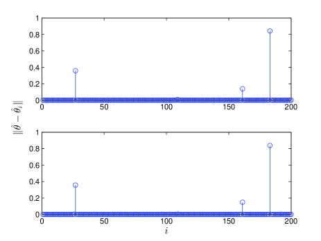
Figure 1: The difference between the estimates of the nominal model parameter $\hat{\theta}$ and the parameter $\hat{\theta}_{i}$ for the $i$th aircraft, $i=1,\cdots,N$. The top plot shows the solution of (6) computed by a centralized algorithm. The plot on the bottom illustrates the distributed solution computed by Algorithm 1. Both the centralized and decentralized solution were computed using a regularization parameter, $\lambda$, set to $150.$

Remark 6.1.

A centralized algorithm for solving (6) would for this example have to solve an optimization problem with 804 optimization variables. If Algorithm 1 is used to distribute the computations, an optimization problem with 8 optimization variables would have to be solved on each system (computer). This comparison illustrates that Algorithm 1 imposes a much cheaper computational cost per iteration on each computer. In addition, the number of optimization variables is invariant to the number of systems and data. Hence, Algorithm 1 provides a computationally tractable and scalable solution to anomaly detection in large homogenous populations.

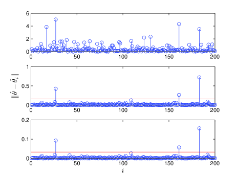
Figure 2: The difference between the estimates of the nominal model parameter $\hat{\theta}$ and the parameter $\hat{\theta}_{i}$ for the $i$th aircraft, $i=1,\cdots,N$. The plots show the solution obtained by the method presented in [11] with regularization parameters 10, 100 and 400, respectively from the top to bottom.

Remark 6.2.

We used 500 flights instead of 5000 flights (5000 flights were used in Example 1 and [11]) to make the estimation problem more challenging. Notice that the anomaly detection problem still leads to a computationally challenging multi-hypothesis problem with roughly $1.3\times 10^{6}$ hypothesis.

7 Conclusion

This paper has presented a novel distributed, scalable and model based approach to anomaly detection for large populations. The motivation for the presented approach is:

• it leads to a scalable approach to anomaly detection that can handle large populations,

• it provides a purely distributed method for detecting anomaly working systems in a collection of systems,

• the method does not require a training data set, and

• the algorithm is theoretically motivated by the results derived in the field of compressive sensing.

The algorithm is based on ideas from system identification and distributed optimization. Basically the anomaly detection problem is first formulated as a sparse optimization problem. This combinatorial multi-hypothesis problem can not be solved for practically interesting sizes of data and a relaxation is therefore proposed. The convex relaxation can be written as a group Lasso problem and theory developed for Lasso and compressive sensing can therefore be used to derive theoretical bounds for when the relaxation is tight.

This work is partially supported by the Swedish Research Council in the Linnaeus center CADICS, the Swedish department of education within the ELLIIT project and the European Research Council under the advanced grant LEARN, contract 267381. Ohlsson is also supported by a postdoctoral grant from the Sweden-America Foundation, donated by ASEA’s Fellowship Fund, and by postdoctoral grant from the Swedish Science Foundation.

References

- [1] B. Abraham and G. E. P. Box. Bayesian analysis of some outlier problems in time series. Biometrika, 66:229–236, 1979.
- [2] B. Abraham and A. Chuang. Outlier detection and time series modeling. Technometrics, 31:241–248, 1989.
- [3] A. Arning, R. Agrawal, and P. Raghavan. A linear method for deviation detection in large databases. In Proceedings of 2nd International Conference of Knowledge Discovery and Data Mining, pages 164–169, 1996.
- [4] M. Basseville and I. V. Nikiforov. Detection of Abrupt Changes – Theory and Application. Prentice-Hall, Englewood Cliffs, NJ, 1993.
- [5] D. P. Bertsekas and J. N. Tsitsiklis. Parallel and Distributed Computation: Numerical Methods. Athena Scientific, 1997.
- [6] S. Boyd, N. Parikh, E. Chu, B. Peleato, and J. Eckstein. Distributed optimization and statistical learning via the alternating direction method of multipliers. Foundations and Trends in Machine Learning, 2011.
- [7] S. Boyd and L. Vandenberghe. Convex Optimization. Cambridge University Press, 2004.
- [8] E. J. Candès, J. Romberg, and T. Tao. Robust uncertainty principles: Exact signal reconstruction from highly incomplete frequency information. IEEE Transactions on Information Theory, 52:489–509, February 2006.
- [9] V. Chandola, A. Banerjee, and V. Kumar. Anomaly detection: A survey. ACM Comput. Surv., 41(15):1–58, July 2009.
- [10] V. Chatzigiannakis, S. Papavassiliou, M. Grammatikou, and B. Maglaris. Hierarchical anomaly detection in distributed large-scale sensor networks. In Proceedings of the 11th IEEE Symposium on Computers and Communications (ISCC’06), pages 761–767, 2006.
- [11] E. Chu, D. Gorinevsky, and S. Boyd. Scalable statistical monitoring of fleet data. In Proceedings of the 18th IFAC World Congress, pages 13227–13232, Milan, Italy, August 2011.
- [12] M. Desforges, P. Jacob, and J. Cooper. Applications of probability density estimation to the detection of abnormal conditions in engineering. Proceedings of Institute of Mechanical Engineers, Part C: Journal of Mechanical Engineering Science, 212:687–703, 1998.
- [13] D. L. Donoho. Compressed sensing. IEEE Transactions on Information Theory, 52(4):1289–1306, April 2006.
- [14] R. O. Duda, P. E. Hart, and D. G. Stork. Pattern Classification (2nd Edition). Wiley-Interscience, 2000.
- [15] E. Eskin. Anomaly detection over noisy data using learned probability distributions. In Proceedings of the Seventeenth International Conference on Machine Learning. Morgan Kaufmann Publishers Inc., pages 255–262, 2000.
- [16] A. J. Fox. Outliers in time series. Journal of the Royal Statistical Society. Series B(Methodological), 34:350–363, 1972.
- [17] D. Gorinevsky, B. Matthews, and R. Martin. Aircraft anomaly detection using performance models trained on fleet data. In 2012 Conference on Intelligent Data Understanding (CIDU), pages 17–23, 2012.
- [18] F. Gustafsson. Adaptive Filtering and Change Detection. Wiley, New York, 2001.
- [19] T. Hastie, R Tibshirani, and J. Friedman. The Elements of Statistical Learning: Data Mining, Inference, and Prediction. Springer Series in Statistics. Springer New York Inc., New York, NY, USA, 10th edition, 2001.
- [20] A. K. Jain and R. C. Dubes. Algorithms for Clustering Data. Prentice-Hall, Inc., 1988.
- [21] L. Ljung. System Identification — Theory for the User. Prentice-Hall, Upper Saddle River, N.J., 2nd edition, 1999.
- [22] L. Parra, G. Deco, and S. Miesbach. Statistical independence and novelty detection with information preserving nonlinear maps. Neural Computing, 8:260–269, 1996.
- [23] R. Patton, P. Frank, and R. Clark. Fault Diagnosis in Dynamic Systems – Theory and Application. Prentice Hall, 1989.
- [24] P. J. Rousseeuw and A. M. Leroy. Robust regression and outlier detection. John Wiley & Sons, Inc., New York, NY, USA, 1987.
- [25] P.-N. Tan, M. Steinbach, and V. Kumar. Introduction to Data Mining. Addison-Wesley, 2005.
- [26] R. Tibsharani. Regression shrinkage and selection via the lasso. Journal of Royal Statistical Society B (Methodological), 58(1):267–288, 1996.
- [27] M. Yuan and Y. Lin. Model selection and estimation in regression with grouped variables. Journal of the Royal Statistical Society, Series B, 68:49–67, 2006.
- [28] J. Zimmermann and G. Mohay. Distributed intrusion detection in clusters based on non-interference. In Proceedings of the 2006 Australasian workshops on Grid computing and e-research – Volume 54, ACSW Frontiers ’06, pages 89–95, Darlinghurst, Australia, 2006.