Nitrogen isotopic ratios in Barnard 1: a consistent study of the N₂H⁺, NH₃, CN, HCN and HNC isotopologues .

Abstract

Context. The ¹⁵N isotopologue abundance ratio measured today in different bodies of the solar system is thought to be connected to ¹⁵N–fractionation effects that would have occured in the protosolar nebula.

Aims. The present study aims at putting constraints on the degree of ¹⁵N–fractionation that occurs during the prestellar phase, through observations of D, ¹³C and ¹⁵N–substituted isotopologues towards B1b. Both molecules from the nitrogen hydride family, i.e. N₂H⁺ and NH₃, and from the nitrile family, i.e. HCN, HNC and CN, are considered in the analysis.

Methods. As a first step, we model the continuum emission in order to derive the physical structure of the cloud, i.e. gas temperature and H₂ density. These parameters are subsequently used as an input in a non–local radiative transfer model to infer the radial abundances profiles of the various molecules.

Results. Our modeling shows that all the molecules are affected by depletion onto dust grains, in the region that encompasses the B1–bS and B1–bN cores. While high levels of deuterium fractionation are derived, we conclude that no fractionation occurs in the case of the nitrogen chemistry. Independently of the chemical family, the molecular abundances are consistent with ¹⁴N/¹⁵N$\sim$300, a value representative of the elemental atomic abundances of the parental gas.

Conclusions. The inefficiency of the ¹⁵N–fractionation effects in the B1b region can be linked to the relatively high gas temperature $\sim$17K which is representative of the innermost part of the cloud. Since this region shows signs of depletion onto dust grains, we can not exclude the possibility that the molecules were previously enriched in ¹⁵N, earlier in the B1b history, and that such an enrichment could have been incorporated into the ice mantles. It is thus necessary to repeat this kind of study in colder sources to test such a possibility.

1 Introduction

Characterizing the nitrogen chemistry is of great interest in studies of star forming regions. Moreover, the possible existence of ¹⁵N–fractionation effects could have strong implications for our understanding of the current solar system. Indeed, large variations have been found in the ¹⁴N/¹⁵N ratio among different solar system bodies (see e.g. Jehin et al., 2009). While this elemental ratio is $\sim$270 on Earth, it is found to be of the order of 450 in the solar wind and Jupiter atmosphere. The latter value is thought to be representative of the protosolar nebula (see e.g. Jehin et al., 2009). Finally, this ratio is in the range 100–150 in cometary ices, as deduced from the analysis of HCN or CN observations. In the coma of comets, most of the CN radicals come from the photodissociation of HCN molecules and, as a consequence, the ¹⁴N/¹⁵N ratios derived from both molecules are necessarily identicals. To date, remote estimates of the nitrogen isotopic elemental ratio in comets only rely on these two molecules. To the contrary, the analysis of the samples of the Stardust mission did not report such high differences. Indeed, the ¹⁴N/¹⁵N ratio was only found to differ by $\sim$20% with respect to the Earth value (Stadermann et al., 2008). An explanation for such a discrepancy could come from a possible enrichment of the HCN molecule in ¹⁵N atoms, due to zero–point chemistry. This would lead to a lower value for the HC¹⁴N/HC¹⁵N ratio compared to the elemental ¹⁴N/¹⁵N ratio. Since the nitriles are not the main career of nitrogen atoms, such a process could reconcile the values obtained from the HCN or CN observations with the in–situ measurements.

Still today, the nitrogen fractionation chemistry is poorly constrained. Pioneering astrochemical models were computed by Terzieva & Herbst (2000) who predicted that the ¹⁵N–enrichment should remain low enough to prevent detection. However, it was subsequently shown by Charnley & Rodgers (2002) and Rodgers & Charnley (2003, 2004, 2008) that, in the regions where CO is highly depleted, the level of fractionation could be high for some species. These models predicted that N₂H⁺ should show the highest degree of fractionation and more generally, that the nitrogen hydride family should be highly fractioned. More recently, Wirström et al. (2012) extended the previous studies and included the dependence on the ortho and para symmetries of H₂ in the chemical network. They showed that, contrary to what was predicted earlier, the nitriles should show the highest degree of fractionation. This latest result is particularly interesting since it would explain the low values obtained for the HC¹⁴N/HC¹⁵N ratio in comets. Additionally, since the nitrogen hydrides, which are the main carriers of nitrogen atoms, are not highly fractioned, this would enable to reconcile the in–situ and remote observations.

Observationally, evidence in favor or against possible fractionation effects are still rare. In part, this comes from the fact that few studies have been dedicated to this problem. Principally, previous works concerned NH₃ (Lis et al., 2010), NH₂D (Gerin et al., 2009), HCN (Dahmen et al., 1995; Ikeda et al., 2002; Hily-Blant et al., 2013), HCN and HNC (Tennekes et al., 2006), HNC and CN (Adande & Ziurys, 2012), or N₂H⁺ (Bizzocchi et al., 2010, 2013). Moreover, most of the studies performed to date focused on a single molecular species (or a combination of two species from the same chemical family), which prevents from distinguishing source–to–source variations of the elemental ¹⁴N/¹⁵N abundance ratio from fractionation effects related to the species under study. Another uncertainty concerns the methodology used. Indeed, many studies rely on the so–called double isotope method in order to retrieve the column density of the main isotopologue, which leads, to some extent, to an uncertainty linked to the value assumed for the fundamental ¹²C/¹³C ratio. Additionally, this method should only work as long as the ¹³C fractionation effects remain small for the species considered.

Here, we focus on the interpretation of rotational lines observed towards B1b for the ¹³C, ¹⁵N and D–substituted isotopologues of N₂H⁺, NH₃, CN, HCN and HNC. This source is located in the Perseus molecular cloud, which has been the subject of many studies. The whole molecular cloud has been mapped, leading to a cartography of its associated extinction (Cernicharo et al., 1985; Carpenter, 2000; Ridge et al., 2006). Additionally, large–scale maps have been obtained of the CO isotopologues (Bachiller & Cernicharo, 1986; Ungerechts & Thaddeus, 1987; Hatchell et al., 2005; Ridge et al., 2006) and of the continuum emission, at various wavelengths (Hatchell et al., 2005; Enoch et al., 2006; Jørgensen et al., 2006). From these studies, it appears that this region contains a large number of active star–forming sites, with a few hundreds of protostellar objects identified. Moreover, it was found that the stars tend to form within clusters. Apart from these extended maps, a large number of dense cores were mapped in other molecular tracers, like NH₃, C₂S (Rosolowsky et al., 2008; Foster et al., 2009), or N₂H⁺ (Kirk et al., 2007).

The source B1b has been the subject of many observational studies, because of its molecular richness. Indeed, many molecules were observed for the first time in this object, like HCNO (Marcelino et al., 2009) or CH₃O (Cernicharo et al., 2012). Additionally, B1b shows a high degree of deuterium fractionation and has been associated with first detections of multiply deuterated molecules, like ND₃ (Lis et al., 2002) or D₂CS (Marcelino et al., 2005). The B1b region was mapped in many molecular tracers, e.g. CS, NH₃, ¹³CO (Bachiller et al., 1990), N₂H⁺ (Huang & Hirano, 2013), H¹³CO⁺ (Hirano et al., 1999), or CH₃OH (Hiramatsu et al., 2010; Öberg et al., 2010). This source consists of two cores, B1–bS and B1–bN, which were first identified by Hirano et al. (1999) and initially classified as class 0 objects. However, since none of these cores seems to be the driving source of molecular outflows (Walawender et al., 2005; Hiramatsu et al., 2010) and because of the properties of their spectral energy distribution (Pezzuto et al., 2012), they may correspond to less evolved objects and were proposed as candidates for the first hydrostatic core stage.

In the present study, we report observations of various isotopologues of N₂H⁺, NH₃, CN, HCN and HNC toward B1b (Sect. 2). In Sect. 3, the analysis of these observations is described. The physical model of the source is based on the analysis of previously published continuum data (Sect. 3.1), which serves as input for the non–local radiative transfer analysis of the molecular data (Sect. 3.2). The current results are then discussed in Sect. 4 and the concluding remarks are given in Sect. 5.

2 Observations

The list of molecular transitions observed as well as the parameters that describe the beam of the telescope at the corresponding line frequencies are summarized in Table 1. Note that this dataset contains previously published data of the NH₃ and NH₂D isotopologues, which are respectively taken from Lis et al. (2010) and Gerin et al. (2009). The central position of the observations is $\alpha$ = 3^h33^m20.90^s, $\delta$ = 31$\degr$07$\arcmin$34.0$\arcsec$ (J2000).

The observations described in this paper have been performed with the IRAM–30m telescope, except for the p-NH₃ and p-¹⁵NH₃ data which were obtained with the Green Bank telescope and described by Lis et al. (2010). The IRAM–30m data have been obtained in various observing sessions in November 2001, August 2004, December 2007, using the heterodyne receivers A100/B100, C150/D150, A230/B230, C270/D270 for spectral line transitions in the 80 – 115 GHz, 130 – 170 GHz, 210 – 260 GHz and 250 – 280 GHz frequency ranges, respectively. The tuning of the receivers was optimized to allow simultaneous observations at two different frequencies simultaneously. These receivers were operated in lower sideband, with a rejection of the upper sideband larger than 15dB. The data obtained at frequencies lower than 80 GHz required a specific calibration, as the receivers were operated in a double sideband mode at these low frequencies. The sideband ratio was calibrated using planets (Mars, Uranus, Neptune) as gain calibrators. The spectra were analysed with the Versatile SPectrometer Array, achieving a spectral resolution ranging from 20kHz for the lower frequency lines (0.07 km s^-1) to 80 kHz (0.09 km s^-1) for the higher frequency transitions like N₂H⁺(3–2). For the weakest lines, the spectra have been smoothed to a spectral resolution of $\sim$0.12 km s^-1 to increase the S/N ratio. We used two observing modes. Frequency switching with a frequency throw of $\sim 7.2$ MHz at 100 and 150 GHz and of $\sim 14.4$ MHz at 230 and 270 GHz, during the 2001 and 2004 observation campaigns (i.e. for the N₂H⁺ and NH₂D maps as well as for the deuterated species). To limit the contamination of the line profiles by baseline ripples and ensure flat baselines, we also used the wobbler switching mode during the 2007 campaign, using a throw of 4$\arcmin$, since the line and continuum maps showed that most of the emission of the B1b core is concentrated in a region of less than 2$\arcmin$.

The pointing was checked on nearby quasars, while we used Uranus for checking the focus of the telescope. The spectra have been calibrated using the applicable forward and main beam efficiencies of 0.95/0.75, 0.93/0.64, 0.91/0.58 , 0.88/0.5 for the A100/B100, C150/D150, A230/B230, C270/D270 mixers respectively. As the radiative transfer model includes the convolution with the telescope beam, we present all spectra in the antenna temperature scale T${}_{A}^{*}$.

The spectra have been processed with the CLASS (Continuum and Line Analysis Single-dish Software) software (www.iram.fr/IRAMFR/GILDAS). We removed linear baselines from the wobbler–switched spectra, while higher order polynomials were necessary for the frequency switched data.

Table 1: Observed line parameters

		$\nu_{\rm 0}$	HPBW	$\eta$	$\delta v$	$\overline{T}_{ex}$	$\tau$
molecule	transition	(GHz)	($\arcsec$)		(km s-1)	(K)
p–NH3	(1,1)	23.694506	33	0.80	0.08	$8.11^{+0.34}_{-0.61}$	6.4
	(2,2)	23.722634	33	0.80	0.08	$8.88^{+0.01}_{-0.01}$	0.3
p–15NH3	(1,1)	22.624929	33	0.80	0.08	7.53	0.02
o–NH2D	$1_{1,1}s-1_{0,1}a$	85.926278	29	0.80	0.14	$6.50^{+0.28}_{-0.45}$	6.4
o–15NH2D	$1_{1,1}s-1_{0,1}a$	86.420128	29	0.80	0.13	5.04	0.02
N2H+	1-0	93.173772	27	0.79	0.13	$6.80^{+0.92}_{-0.40}$	8.3
	3-2	279.511858	9	0.57	0.08	$5.82^{+1.38}_{-0.91}$	5.7
N2D+	1-0	77.109622	32	0.83	0.08	$8.41^{+0.45}_{-0.45}$	1.7
	3-2	231.321857	10	0.60	0.05	$6.42^{+0.32}_{-0.39}$	2.3
15NNH+	1-0	90.263833	28	0.80	0.13	$5.78^{+0.00}_{-0.00}$	0.03
N15NH+	1-0	91.205741	28	0.80	0.13	$5.73^{+0.00}_{-0.00}$	0.03
HCN	1-0	88.631847	29	0.79	0.13	$5.77^{+2.35}_{-1.65}$	55.6
	2-1	177.261222	14	0.69	0.07	$4.90^{+1.33}_{-1.35}$	89.7
	3-2	265.886499	9	0.57	0.05	$4.42^{+0.57}_{-0.92}$	36.9
H13CN	1-0	86.340163	29	0.79	0.14	$3.28^{+0.13}_{-0.10}$	4.2
	2-1	172.677956	14	0.69	0.07	$3.11^{+0.11}_{-0.13}$	3.2
	3-2	259.011866	9	0.60	0.18	$3.45^{+0.10}_{-0.10}$	0.4
HC15N	1-0	86.054966	29	0.79	0.14	$3.18^{+0.00}_{-0.00}$	0.9
	2-1	172.107957	14	0.69	0.07	$3.07^{+0.00}_{-0.00}$	0.6
	3-2	258.156996	9	0.60	0.05	$3.47^{+0.00}_{-0.00}$	0.1
DCN	1-0	72.414933	34	0.84	0.08	$4.53^{+0.44}_{-0.24}$	3.3
	2-1	144.828111	17	0.69	0.08	$3.71^{+0.38}_{-0.38}$	4.9
	3-2	217.238612	11	0.64	0.05	$3.79^{+0.23}_{-0.29}$	1.4
D13CN	3-2	213.519936	12	0.66	0.11	$4.04^{+0.09}_{-0.05}$	0.8
HNC	1-0	90.663568	28	0.79	0.13	$8.29^{+0.21}_{-0.24}$	8.6
	3-2	271.981142	9	0.60	0.09	$6.58^{+0.04}_{-0.06}$	11.7
HN13C	1-0	87.090850	29	0.79	0.13	$5.84^{+0.07}_{-0.07}$	0.8
	2-1	174.179408	14	0.69	0.13	$4.51^{+0.02}_{-0.03}$	1.2
	3-2	261.263310	9	0.60	0.05	$4.37^{+0.02}_{-0.02}$	0.3
H15NC	1-0	88.865717	28	0.79	0.13	$6.05^{+0.00}_{-0.00}$	0.2
	2-1	177.729094	14	0.69	0.13	$4.42^{+0.00}_{-0.00}$	0.3
	3-2	266.587800	9	0.60	0.18	$4.62^{+0.00}_{-0.00}$	0.06
DNC	2-1	152.609737	16	0.69	0.08	6.98	7.0
	3-2	228.910489	11	0.66	0.05	5.06	5.0
DN13C	2-1	146.734002	17	0.69	0.16	3.96	0.4
	3-2	220.097238	11	0.66	0.05	3.92	0.1
CN	1-0	113.490982	21	0.79	0.20	$4.62^{+1.57}_{-0.50}$	34.5
	2-1	226.874781	11	0.66	0.11	$3.86^{+1.29}_{-0.67}$	47.6
13CN	1-0	108.780203	21	0.79	0.21	$3.42^{+0.03}_{-0.01}$	1.6
	2-1	217.467150	11	0.64	0.11	$3.43^{+0.03}_{-0.02}$	0.8
C15N	1-0	110.024590	21	0.79	0.11	$3.39^{+0.01}_{-0.00}$	0.3

Note.– Summary of the nitrogen containing species observed at the IRAM telescope (except for the NH₃ isotopologues that were observed at the Green Bank Telescope). The NH₃ and NH₂D isotopologue observations are respectively taken from Lis et al. (2010) and Gerin et al. (2009). All the observations were obtained at a single position except for N₂H⁺ J=1-0 and NH₂D, for which we obtained maps. For each line, we indicate the central frequency of the line ($\nu_{0}$) as well as the quantum numbers of the corresponding transition. The HPBW and efficiency ($\eta$) of the the telescope at this frequency and the spectral resolution ($\delta\nu$) of the observations are also indicated. The two last columns indicate the averaged excitation temperature and the opacity of the rotational lines (summed over the hyperfine components), as derived from the results of the radiative transfer modeling. The upper/lower subscripts for $\overline{T}_{ex}$ indicate the highest/lowest excitation temperatures found when considering all the hyperfine components. These quantities are zero when all the hyperfine components are described by the same excitation temperature. In the case of the DNC isotopologues, we neglected the hyperfine structure and the subscripts are thus absent.

3 Continuum and molecular line modelling

The distance of the source is taken to be 235 pc (Hirota et al., 2008). At this distance, an angular size of 10$\arcsec$ corresponds to a physical size of 0.0114 pc.

3.1 Continuum

In order to derive the gas temperature and H₂ density profiles, we used continuum observations at $\lambda$ = 350 $\mu$m and $\lambda$ = 1.2 mm, respectively obtained at the CSO and IRAM telescopes. The corresponding continuum maps are reported in Fig. 1 and 2. In these figures, we indicate the positions of the B1–bS and B1–bN cores identified by Hirano et al. (1999) as well as the Spitzer source [EDJ2009] 295 ($\alpha$ = 03^h33^m20.34^s ; $\delta$ = 31$\degr$07$\arcmin$21.4$\arcsec$ (J2000)) referenced in Jørgensen et al. (2006) and Evans et al. (2009).

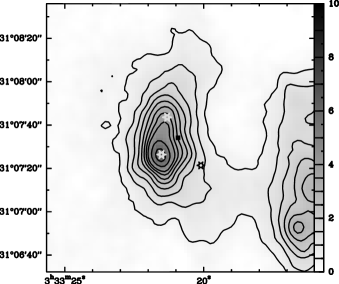
Figure 1: Continuum map at 350 $\mu$m obtained at the CSO with the SHARC instrument. The contours have a step of 0.5 Jy/beam from 0.5 to 4 Jy/beam and 1 Jy/beam for larger fluxes, as drawn on the right. The white stars indicate the position of B1–bS and B1–bN and the black star corresponds to the Spitzer source [EDJ2009] 295. The black dot gives the position of our molecular survey.

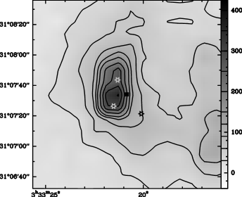
Figure 2: Same as Fig. 2 but for the 1.2 mm continuum observed at the IRAM telescope with the MAMBO instrument. The contours have a step of 30 mJy/beam from 30 to 150 mJy/beam and 50 mJy/beam for higher fluxes, as drawn on the lookup table on the right.

The peak position of the 1.2 mm observations is found at $\alpha$ = 03^h33^m21.492^s ; $\delta$ = 31$\degr$07$\arcmin$32.87$\arcsec$ (J2000), which is offset by (+8$\arcsec$,-1$\arcsec$) with respect to the position of the molecular line observations given in Sect. 2. The 350 $\mu$m observations peak at the B1–bS position and is thus offset by $\sim$6$\arcsec$ to the south–south west, with respect to the 1.2 mm peak position. In the modeling, we assumed that the central position of the density distribution is half–way between the 350 $\mu$m and 1.2 mm peaks, which corresponds to the coordinates $\alpha$ = 03^h33^m21.416^s ; $\delta$ = 31$\degr$07$\arcmin$29.79$\arcsec$ (J2000). In order to characterize the continuum radial behaviour, we performed an annular average of the map around this position. In the B1 region, there are two other cores, labelled B1–d and B1–c by Matthews & Wilson (2002), which are respectively offset by $\sim$80$\arcsec$ to the SW and $\sim$125$\arcsec$ to the NW from the central position. While performing the average, we discarded the points distant by less than 30$\arcsec$ from these two cores. The fluxes defined in this way are represented in Fig. 3 and the error bars represent one standard deviation, $\sigma$.

3.1.1 Modelling

In order to infer the radial structure of the source from these observations, we performed calculations using a ray–tracing code. As an input, we fix the H₂ density and temperature profiles which gives, as an output, the intensity as a function of the impact parameter. The model predictions are then compared to the observations by convolving with the telescopes beams, which are respectively approximated by Gaussians of 9$\arcsec$ and 15$\arcsec$ FWHM for the CSO and IRAM telescopes.

As a starting point, we performed a grid of models assuming that the source is isothermal. We fixed the dust temperature at $T_{d}$ = 12K, which is the typical temperature of the region, according to the analysis of NH₃ observations reported by Bachiller et al. (1990) or Rosolowsky et al. (2008). We parametrized the density profile as a series of power laws, i.e :

$$n_{0}(r) =n_{0} \quad r<r_{0}$$ if (1)

$$n_{i}(r) =n_{i-1}(r_{i-1})\times\left(\frac{r_{i-1}}{r}\right)^{\alpha_{i}} \quad r_{i-1}<r<r_{i}$$ if (2)

and we computed a grid of models with the following parameters kept fixed : $r_{0}$ = 5$\arcsec$, $r_{1}$ = 35$\arcsec$, $r_{2}$ = 125$\arcsec$, $r_{3}$ = 450$\arcsec$ and $\alpha_{3}$ = 3.0. The density profile is thus described by three free parameters, the central H₂ density $n_{0}$, and the slopes of the first and second regions, $\alpha_{1}$ and $\alpha_{2}$. This choice is based on some preliminary models, for which we found that these delimiting radii were accurate in order to reproduce the morphology of the SED. Moreover, the slope of region 3 was found to be poorly constrained which motivated us to keep it fixed.

The dust absorption coefficient is parametrized according to

$$\kappa_{abs}(\lambda)=\kappa_{1300}\left(\frac{1300}{\lambda}\right)^{\beta}$$ (3)

with $\lambda$ expressed in $\mu$m and $\kappa_{1300}$ being the absorption coefficient at 1.3 mm. Values for the dust absorption coefficient were determined by Ossenkopf & Henning (1994), for the case of dust grains surrounded by ice mantles. The values were found to be in the range $0.5<\kappa_{1300}<1.1$ cm²/g, where $\kappa_{1300}$ is given in function of the dust mass. Hence, we fixed the gas–to–dust mass ratio to 100 and furthermore fixed the absorption coefficient to $\kappa_{1300}$ = 0.005 cm²/g, where $\kappa_{1300}$ is this time refereed to the mass of gas. The results of the models depend only on the product $\kappa_{1300}\times n_{0}$. The grid is then computed considering $\beta$ as an additional free parameter.

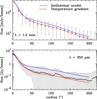
Figure 3: Comparison of the observed and model fluxes as a function of radius at 350 $\mu$m (bottom panel) and 1.2 mm (upper panel). The blue curve corresponds to a model obtained assuming that the source is isothermal at T_d=12K. The red curve corresponds to a model where we introduced a temperature gradient.

From the results of the grid, it appears that the best models are found for parameters in the range : $3\,10^{6}<n_{0}<6\,10^{6}$ cm^-3, $2.0<\alpha_{1}<2.4$, $1.2<\alpha_{2}<1.5$ and $1.7<\beta<2.4$. However, we could not find a model that would fit satisfactorily the radial profiles at both wavelengths. The origin of the problem is illustrated in Fig. 3. In this figure, the blue curve corresponds to a model that satisfactorily reproduces (i.e. within 30%) the 1.2 mm radial profile. It can be seen that this model is able to reproduce the flux at 350 $\mu$m, for radii $r<20\arcsec$. However, for larger radii, the flux is overestimated by a factor 3. Obviously, such a radial dependence cannot be accounted for by a modification of the $n_{0}$, $\kappa_{1300}$ or $\beta$ parameters, since changes in these parameters would modify the relative fluxes at both wavelengths and independently of the radius.

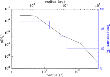
Figure 4: Temperature (blue curve, right axis) and H₂ density (black curve, left axis) derived from the SED fitting.

A solution to this problem is to introduce a temperature gradient in the model. Indeed, an increase of the dust temperature will affect differently the fluxes at 350 $\mu$m and 1.2 mm, producing a larger increase at the shorter wavelength. We thus modified the best model obtained from the grid analysis by introducing a gradient in the dust temperature, from 17K in the center to 10K in the outermost region. The resulting fit is shown by the red curve in Fig. 3. The parameters of this model are $n_{0}=3\,10^{6}$ cm^-3, $\alpha_{1}=2$, $\alpha_{2}=1.2$ and $\beta=1.9$. The dust temperature and H₂ density are represented in Fig. 4. With the density profile defined this way, the peak value of the H₂ column density is N(H₂) = $2.1\,10^{23}$ cm^-2. The average column density, within a 30$\arcsec$ FWHM beam, is N(H₂) = $7.6\,10^{22}$ cm^-2, in good agreement with the estimate of Johnstone et al. (2010), i.e. N(H₂) = $8.2\,10^{22}$ cm^-2, obtained assuming the same beam. The FHWM of the column density distribution is $\sim$16$\arcsec$. Finally, the current density profile corresponds to enclosed masses of 0.5, 1.8, 4.5 and 13.1 M_☉ for delimiting radii of 10, 30, 60 and 120$\arcsec$, respectively ($\sim$ 0.01, 0.03, 0.07 and 0.14 pc, assuming a distance to B1 of 235 pc).

3.1.2 Comparison with previous studies

B1b has been the subject of many studies with both ground– and space–based telescopes. In particular, interferometric observations by Hirano et al. (1999) lead to the identification of two cores, separated by $\sim$20$\arcsec$ and designated as B1–bS and B1–bN. These objects are respectively offset by (+6$\arcsec$,-7$\arcsec$) and (+5$\arcsec$,+10$\arcsec$) with respect to the central position of our observations (see Sect. 2) and are thus both at a projected distance $\sim$10$\arcsec$. By modelling the SED from 350 $\mu$m to 3.5 mm, these authors found that both objects can be characterized by a dust temperature of T_d = 18K, with a density distribution consistent with $n(r)$ $\propto$ r^-1.5 and without central flattening. They estimated the bolometric to submm luminosities to $L_{bol}/L_{submm}$ $\sim$ 10, well below the limit of 200 for class 0 objects (Andre et al., 1993). Thus, these characteristics would suggest that the two sources are very young class 0 objects.

Recently, Pezzuto et al. (2012) characterized B1–bS and B1–bN by combining Spitzer, Herschel and ground–based observations. The modelling of the SEDs showed that the two objects are more evolved than prestellar cores, but have not yet formed class 0 objects. In particular, the non-detection of B1–bS at 24 $\mu$m and detection at 70 $\mu$m place this source as a candidate for the first hydrostatic core stage. However, the bolometric luminosity of this source, estimated as $L_{bol}$ $\sim$ 0.5 L_☉ is above the limit of 0.1 L_☉ that characterizes the maximum luminosity at this evolutionary stage (Omukai, 2007). The non–detection of B1–bN at these two wavelengths gives this source the status of a less evolved object. Pezzuto et al. (2012) described these objects by using a combination of blackbody plus modified–blackbody components, that respectively characterize the central object and the surrounding dust envelope. For the two objects, the central temperature was found to be of the order of 30K and the envelope has a typical temperature $\sim$ 9K. However, as noted by these authors, in a realistic model, the emission of the central object will be absorbed by the dusty envelope which will lead to a stratification in the dust temperature.

Even more recently, Huang & Hirano (2013) presented 1.1 mm continuum interferometric maps of the B1b region where the B1-bS and B1-bN objects are spatially resolved. For those two objects, they quote the parameters from the upcoming work by Hirano et al. (2013) that describe the fit of the SED. B1-bS and B1-bN are respectively described by indexes $\beta=1.3\pm 0.2$ and $1.8\pm 0.4$ and T_d = $18.6\pm 1.6$ K and $15.6\pm 2.2$ K.

3.2 Molecular excitation modeling

The line radiative transfer (RT) is solved using the short–characteristics method and includes line overlap for the molecules with hyperfine structure. The underlying theory and numerical code are described in Daniel & Cernicharo (2008). For most of the molecules, the spectroscopy is retrieved from the splatalogue database which centralizes the spectroscopic data available in other databases like JPL (Pickett et al., 1998) or CDMS (Müller et al., 2001, 2005). The rate coefficients are retrieved from the BASECOL database (Dubernet et al., 2013). The references for both the spectroscopy and collisional rate coefficients are further described in what follows when considering the individual molecules. In the case of linear molecules that have a hyperfine structure resolved by the observations, but for which the collisional rate coefficients just take into account the rotational structure (e.g. the HNC isotopologues), we emulate hyperfine rate coefficients using the IOS–scaled method described in Neufeld & Green (1994). It has been shown by Faure & Lique (2012) that this method of computing hyperfine rate coefficients leads to accurate results when compared to rate coefficients obtained with a more accurate recoupling scheme. In the case of the symmetric or asymmetric tops (i.e. NH₃ and NH₂D), the hyperfine rate coefficients are obtained using the M–random method. Moreover, in the case of collisional systems that consider He as collisional partner, we scale the rate coefficients in order to emulate rate coefficients with H₂, using a scaling factor that depends on the ratio of the reduced masses of the two colliding systems. The same approximation is used to determine the rate coefficients of the rarest isotopologues.

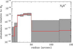
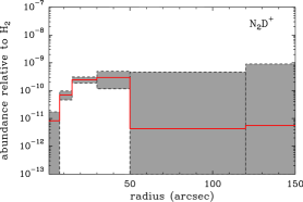
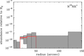
Figure 5: Abundance profiles of the N₂H⁺ isotopologues derived from the modeling (red lines). The shaded areas give a confidence zone for the abundance as delimited by the lower and upper boundaries in each region (see Sect. 3.2 for details).

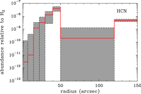
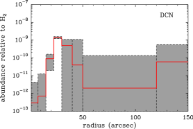
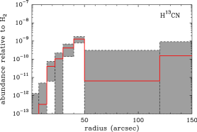
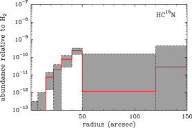
Figure 6: Abundance profiles of the HCN isotopologues derived from the modeling.

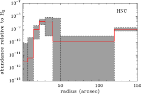
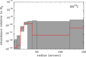
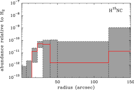
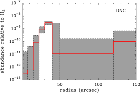
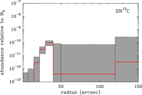
Figure 7: Abundance profiles of the HNC isotopologues derived from the modeling.

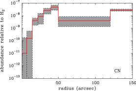
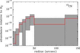
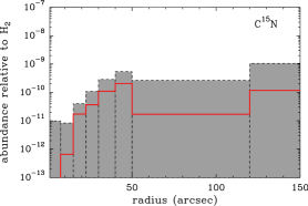
Figure 8: Abundance profiles of the CN isotopologues derived from the modeling.

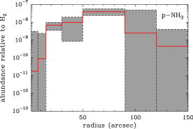
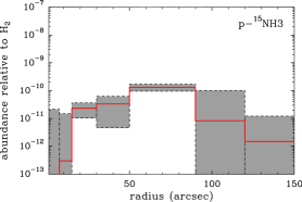
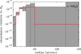
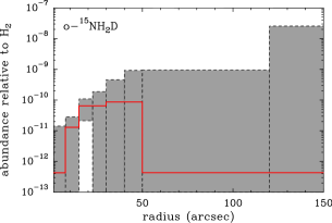
Figure 9: Abundance profiles of the NH₃ isotopologues derived from the modeling.

Table 2: Column densities and isotopic ratios derived from the modelling

	log(N)	ratio to main related isotopologue		ratio with 12C/13C = 60
p–NH3	14.74${}^{+0.25}_{-0.13}$		…
p–15NH3	12.25${}^{+0.43}_{-0.08}$	NH3/15NH3 =	300${}^{+55}_{-40}$
o–NH2D	14.73${}^{+0.12}_{-0.08}$		…
o–15NH2D	12.37${}^{+0.33}_{-0.11}$	NH2D/15NH2D =	230${}^{+105}_{-55}$
N2H+	13.48${}^{+0.04}_{-0.04}$		…
N2D+	13.02${}^{+0.18}_{-0.07}$	N2H+/N2D+ =	2.9${}^{+0.5}_{-1.0}$
15NNH+	$<$ 10.69	N2H+/15NNH+	$>600$
N15NH+	10.88${}^{+0.50}_{-0.11}$	N2H+/N15NH+ =	400${}^{+100}_{-65}$
HCN	14.40${}^{+0.09}_{-0.10}$		…
H13CN	12.91${}^{+0.19}_{-0.10}$	HCN/H13CN =	30${}^{+7}_{-4}$
HC15N	12.18${}^{+0.42}_{-0.10}$	HCN/HC15N =	165${}^{+30}_{-25}$	330${}^{+60}_{-50}$
DCN	13.08${}^{+0.31}_{-0.09}$	HCN/DCN =	20${}^{+6}_{-10}$	40${}^{+12}_{-20}$
D13CN	$<12.38$	DCN/D13CN	$>5$
HNC	13.77${}^{+0.14}_{-0.13}$		…
HN13C	12.47${}^{+0.37}_{-0.14}$	HNC/HN13C =	20${}^{+5}_{-4}$
H15NC	11.90${}^{+0.33}_{-0.14}$	HNC/H15NC =	75${}^{+25}_{-15}$	225${}^{+75}_{-45}$
DNC	13.31${}^{+0.16}_{-0.10}$	HNC/DNC =	2.9${}^{+1.1}_{-0.9}$	$9^{+3}_{-3}$
DN13C	11.84${}^{+0.51}_{-0.14}$	DNC/DN13C =	30${}^{+8}_{-5}$
CN	14.78${}^{+0.05}_{-0.05}$		…
13CN	13.08${}^{+0.19}_{-0.14}$	CN/13CN =	50${}^{+19}_{-11}$
C15N	12.40${}^{+0.51}_{-0.14}$	CN/C15N =	240${}^{+135}_{-65}$	290${}^{+160}_{-80}$

Note.– Unconvolved column densities obtained from the modeling of the various molecules. The ratio of the rarest isotopologues with respect to the main one are also given.

or singly ¹³C– or ¹⁵N– or D– substituted isotopologue, the column density ratio corresponds to N(main) / N(singly subtituted). For doubly substituted isotopologues (wether ¹³C– and D– or ¹⁵N– and D– substituted), the ratio correspond to N(D– substituted) / N(doubly substituted)

In the modeling, the center of the density distribution corresponds to the one adopted when modeling the continuum radial profiles and is given is Sect. 3.1. The offset with the position of the molecular line observations is accounted for by computing the molecular spectra at a projected distance of 8$\arcsec$ from the center. The abundance of a given molecule is obtained dividing the radial profile in a maximum of eight regions. These regions are chosen as a sub–division of the regions chosen to describe the temperature profile. Additionally, for each molecular species, the grid is defined to minimize the abundance variations between two consecutive shells. The outermost radius considered in the model, for all the molecules, is 450$\arcsec$. However, in Fig. 5–9 where the abundances that result from the modelling are plotted, we truncate the radius at 150$\arcsec$ since the abundance is constant outside 120$\arcsec$. The abundance in each region is then determined using a Levenberg-Marquardt algorithm, which searches for the best value of the abundances on the base of a $\chi^{2}$ minimization. Typically, a solution is found in 20–30 iterations. In the case of the ¹³C and ¹⁵N isotopologues, the fit is performed simultaneously with the main isotopologue. We force the abundance profiles of the various isotopologues to be identical within a scaling factor. In the case of the D–substituted isotopologues, we impose that the abundance in every region is in the range $\chi$(HX)/1000 $<$ $\chi$(DX) $<$ $10\times\chi$(HX).

For N₂H⁺ and o–NH₂D, the abundance profiles are better constrained because of the availability of emission maps, which is not the case for the other molecules. From the models computed for o–NH₂D and N₂H⁺, it appears, however, that the abundance profile derived just using the observations at the central position should give reliable abundance profiles. The main uncertainty would concern the balance of the molecular abundance between consecutive shells. However, the global shape of the abundance profile would remain qualitatively unchanged. The fact that the abundance profile is sensitive to observations at a single position comes from the steepness of the density/temperature profile, in conjunction with the availability of multiple lines for a single species with different critical densities.

The error bars of the abundances are obtained by considering each region separately. For each region, the upper and lower limit of the abundance are set so that the $\chi^{2}$ does not exceed a given threshold. This way of computing the error bars does not account for the inter–dependence of the different regions, but gives indications of the influence of each region on the emergent intensities. For each molecule, the best abundances are represented in Fig. 5, 6, 7, 8 and 9 as red lines. The grey regions correspond to the range of abundances delimited by the upper and lower limits. In the figures that compare the observed and modeled spectra, the grey regions correspond to line intensity uncertainties expected from the error bars set on the abundances. From the results of the non–local radiative transfer modeling, we calculate for each molecular line an averaged excitation temperature $\overline{T}_{ex}$, as well as the line center opacity. These quantities are given in Table 1. The averaged excitation temperature is calculated by taking into account the regions of the cloud that contribute to the emerging line profile, the average being given by Eq. (2) of Daniel et al. (2012).

The N₂H⁺ maps of Huang & Hirano (2013) show that the B1–bS and B1–BN cores have different V_LSR, B1–bS being at 6.3 km s^-1 and B1–bN at 7.2 km s^-1. In the present observations, the B1–bN component appears as a redshifted shoulder in the spectra of some species. However, with the current angular resolutions, it is impossible to disentangle the exact contributions of the two emitting cores, since they spatially overlap. Additionally, our model is 1D spherical, which does not allow us to describe in detail the complexity of this region. We thus assumed a single V_LSR $\sim$ 6.7 km s^-1. For some molecules, like N₂H⁺ or NH₃, the individual hyperfine component have symmetric shapes and with this assumption, it is possible to obtain an overall good fit of the lines. However, for HCN or HNC, the emission at 7.2 km s^-1 is strong and this assumption is no longer valid. In such cases, we have chosen to calculate the $\chi^{2}$ just considering the blue part of the lines. The channels used to calculate the $\chi^{2}$ are shown as black thick histograms in the figures that compare the models to the observations.

In the model, we introduce two regions in terms of infall velocity and turbulent motion. The infall velocity in the region with $r<120\arcsec$ was set to 0.1 km s^-1 and the turbulent motion to 0.4 km s^-1. These values were chosen since they reproduce the widths of the molecular lines, as well as the asymmetry seen in some molecular lines, e.g. in the HNC or HCN spectra. Outside 120$\arcsec$, the gas is considered to be static and the turbulent motion is increased to 1.5 km s^-1 in order to reduce the emerging intensities of the HCN and HNC lines. Indeed, with such a high turbulence, the lines are absorbed but no self–absorption features are seen in the synthesized spectra. Thus, this enables to increase the amount of absorbing material to a larger extent than it would be possible by simply fitting the observed self–absorption features. Consequently, this allows to increase the column density of the main isotopologues with respect to the ¹³C isotopologues since the latter are less affected by self–absorption effects. This is motivated by the fact that we derive low HCN/H¹³CN and HNC/HN¹³C column density ratios by compared to isotopic ratios in local interstellar medium (see Sect. 3.4). Moreover, such an assumption is reasonable in view of the observations related to the Perseus molecular cloud. Indeed, Kirk et al. (2010) showed that the turbulent motion in this region follows the Larson’s law (Larson, 1981), with a turbulent motion that increases with the distance to the core center and typically reaches a value of 1 km s^-1 at a linear scale of 1 pc. Finally, we emphasize that this outermost region of the model is poorly constrained by the data and its parameters should be treated with caution and seen as averaged values that would describe the overall foreground material.

Finally, in Table 2, we give the column densities of all the molecular species considered in this study, as well as the column density ratio of the rarest isotopologues with respect to the main ones. Since for a given species, the models are based on various lines observed with different spatial resolutions, we give column densities which simply correspond to an integration along the diameter of the sphere and which are not convolved with any telescope beam.

3.3 N₂H⁺

3.3.1 Spectroscopy and collisional rate coefficients

The spectroscopic coupling constants for the hyperfine structure of N₂H⁺ are taken from Caselli et al. (1995). We adopt the scaling of the rotational constants described in Pagani et al. (2009), where the way we calculate the line strengths is also described. In the case of the ¹⁵N isotopologues, the hyperfine structure due to the ¹⁵N nucleus is not resolved. In this case, we just introduce in the spectroscopy the spin of the ¹⁴N nucleus. The coupling constants are from Dore et al. (2009) and we use the same methodology as Pagani et al. (2009) in order to derive the line strengths of the two isotopologues.

The collisional rate coefficients are from Daniel et al. (2005) and consider He as a collisional partner. In the case of the ¹⁵N isotopologues, these rate coefficients are also used but we apply the recoupling method to one nuclear spin.

3.3.2 Results

In the case of N₂H⁺, in addition to the observations of the $J$=1–0 and 3–2 lines at the central position, the abundance profile is constrained by taking into account the $J$=1–0 map shown in Fig. 11. To do so, we compute the integrated intensity over the hyperfine components for each position of the map. These integrated intensities are then averaged radially and the $\chi^{2}$ is calculated by taking into account both the central position and the integrated intensity radial profile.

The various abundance profiles derived from the modeling are shown in Fig. 5. The comparison of the observations with the modeled line profiles is shown in Fig. 10 and the map of the $J$=1-0 observations is compared with the model in Fig. 11. The column densities for each isotopologue, as well as the column density ratios, are given in Table 2.

3.3.3 Comparison with previous studies

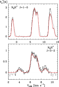
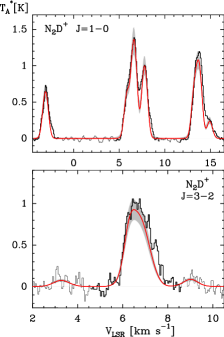
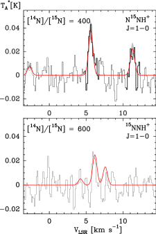
Figure 10: Observed (histograms) and modeled (red lines) spectra for (a) N₂H⁺ ($J$=1-0) (top panel) and N₂H⁺ ($J$=3-2) (bottom panel) (b) N₂D⁺ ($J$=1-0) (top panel) and N₂D⁺ ($J$=3-2) (bottom panel) (c) N¹⁵NH⁺ ($J$=1-0) (top panel) and ¹⁵NNH⁺ ($J$=1-0) (bottom panel). The shaded areas correspond to the variations expected from the error-bars set on the abundance profiles and represented in Fig. 5.

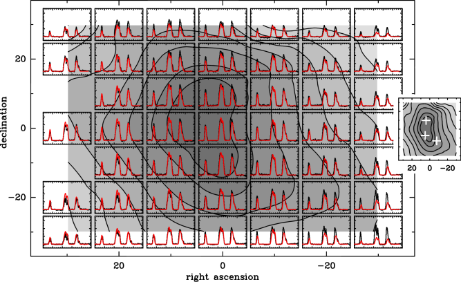
Figure 11: Map of the observed (histograms) and modeled (red lines) spectra of N₂H⁺ ($J$=1–0). The background corresponds to a map of the iscocontours of the intensity integrated over all the hyperfine components. The map on the right side shows the isocontours with the same scale for the right ascension and declination. The white crosses indicate the position of the B1–bN and B1–bS sources identified by Hirano et al. (1999), as well as the Spitzer source reported by Jørgensen et al. (2006).

Kirk et al. (2007) have previously reported N₂H⁺ maps of the whole Perseus molecular cloud and various studies focused on a sample of prestellar or protostellar cores in this region (Roberts & Millar, 2007; Emprechtinger et al., 2009; Johnstone et al., 2010; Friesen et al., 2013). Additionally, a few studies were specifically devoted to the B1b region (Gerin et al., 2001; Huang & Hirano, 2013). The column density estimates range from $\sim$$10^{13}$ to $4.5\,10^{13}$ cm^-2 and the current estimate of $\sim$$3\,10^{13}$ cm^-2 thus falls between the previous ones.

Moreover, the N₂D⁺/N₂H⁺ column density ratio was estimated in various studies. This ratio was found to be 0.15 by Gerin et al. (2001), 0.25 by Roberts & Millar (2007), 0.18 by Emprechtinger et al. (2009) and 0.1 by Friesen et al. (2013). More recently, from interferometric observations, Huang & Hirano (2013) estimated the ratio in the B1–bS and B1–bN cores and derived values of 0.13 and 0.27 towards those two positions. In the current study, we obtain a column density ratio $\sim$0.34 at the core center, a value higher than all the previous estimates.

Part of the differences comes from the assumptions made in the respective analysis. Prior to this work, the analysis was carried out using the assumption of local thermodynamic equilibrium (hereafter referred to as LTE approach and the details related to this method can be found in e.g. Caselli et al., 2002) and in most cases, the same excitation temperature was assumed for the two isotopologues. In the current model, by considering the excitation temperatures given in Table 2, we can see that this assumption is true within 20% and 10% for the $J$=1–0 and $J$=3–2 lines respectively. While this might not lead to substantial errors in the column density estimate, if based on the $J$=1–0 line, the error can however be larger for the $J$=3–2 line, since the $J$=3 energy level is at $\sim$26K. We refer the reader to the discussion performed in the o–NH₂D case, given in Sect. 3.6, for further details. Finally, from the current model, we infer that the average excitation temperature of N₂D⁺ is higher than that of N₂H⁺, which is a consequence of a more centrally peaked distribution of $\chi$(N₂D⁺) compared to $\chi$(N₂H⁺). On the other hand, the excitation temperatures of the two ¹⁵N isotopologues of N₂H⁺ are lower than that of N₂H⁺. This comes from different line trapping effects. Thus, detailed radiative transfer models are required in order to interpret accurately the line intensities.

Additionally, regardless from the method of analysis, the models show that the respective abundances of N₂D⁺ and N₂H⁺ strongly vary with radius. Indeed, in the innermost region, i.e. $r<15\arcsec$, we obtain $\chi$(N₂D⁺)/$\chi$(N₂H⁺) larger than unity, while for greater radii, this ratio falls below 0.1. This radial variation of the two isotopologue abundances explains, to some extent, the dispersion in the column density ratio estimates. The reason is that the various studies were not all based on the same observational position and moreover, the telescope beams were not necessarily similar. The strong radial variations of $\chi$(N₂D⁺)/$\chi$(N₂H⁺) thus make beam dilution effects an important factor when estimating the column density ratio.

The abundance profiles we derive for N₂H⁺ and N₂D⁺ (given in Fig. 5) show that for $r<15^{\prime\prime}$ (the region that encloses both B1–bS and B1–bN), the abundance of these species are reduced respectively by factors $\sim$100 and 10, with respect to the maximum abundances which are found at radii $15\arcsec<r<50\arcsec$. On the other hand, the interferometric maps of Huang & Hirano (2013) show that the peak intensities of the N₂H⁺($J$=3-2) and N₂D⁺($J$=3-2) maps are found at the positions of the B1–bN and B1–bS sources. Both findings may seem incompatible. It is thus important to emphasize the fact that even if the N₂H⁺ and N₂D⁺ abundance profiles show signs of depletion in the current analysis, the abundance is still high enough in this depleted region for the lines to be sensitive to the gas density, especially in the excited rotational lines. In other words, despite of the low abundances, the $J$=3-2 lines will still trace the density enhancements. This can be seen when considering the upper boundaries of the abundance represented in Fig. 5. Indeed, the upper limits of the N₂H⁺ and N₂D⁺ abundances in the region $r<15\arcsec$ are still factors $>$10 and $>$5 below the maximum abundances found at $15\arcsec<r<50\arcsec$. This is further illustrated by the fact that the synthetic map of the N₂H⁺ $J$=3-2 emission shown in Fig. 12 has a maximum in the inner $15\arcsec$ region.

Additionally, we recall that the description of the innermost part of the B1b region is just a crude approximation of the exact geometry of the source, and a quantitative estimate of the amount of depletion would require a more detailed analysis, preferentially based on a 3D modeling of the region. Indeed, this point is illustrated in Fig. 12 where a synthetic map of the N₂H⁺ $J$=3–2 emission is shown. This map is obtained assuming a FWHM telescope beam of 4$\arcsec$, which corresponds to the angular resolution of the map shown in Fig. 2 (c) of Huang & Hirano (2013). Compared to the interferometric map of Huang & Hirano (2013), we see that the current model can reproduce, at least qualitatively, the radial variation of the $J$=3–2 intensity for radii r $>$ 20$\arcsec$. However, the maximum integrated intensity predicted by the current model is 2 Jy km s^-1/beam, and the integrated intensity is roughly constant within the central 15$\arcsec$. On the other hand, the interferometric map shows that at the positions of B1–bS and B1–bN, the intensity can reach values of $\sim$3 Jy km s^-1/beam, and is above 2 Jy km s^-1/beam close to these sources, in a filament that connects the two objects. The current model is thus reliable enough to describe the envelope at large scales, but fails to mimic the complexity of the B1b region in the vicinity of the B1–bS and B1–bN sources. To account for the geometry of the H₂ density distribution, it would be necessary to adopt a 3D model.

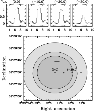
Figure 12: Simulated map of the N₂H⁺ $J$=3–2 integrated intensity as seen by a telescope of synthesized beam size of 4$\arcsec$ (bottom panel). This map can be directly compared to the map given in Fig. 2 (c) of Huang & Hirano (2013). The three isocontours shown are 0.51, 1.02 and 1.53 Jy km s^-1/beam as in Huang & Hirano (2013). The large crosses indicate the positions of B1–bN and B1–bS. The upper panels shows line profiles as a function of the distance from the center. The corresponding positions are indicated by small crosses on the map. The velocity resolution of the spectra is 0.3 km s^-1.

The N₂D⁺/N₂H⁺ column density ratio is mainly influenced by the abundance of the deuterated isotopologues of H${}_{3}^{+}$, whose abundances will be mainly governed by two processes. The first one is linked to the amount of CO that remains in the gas phase. Indeed, if CO is abundant, it will preferentially react with the H${}_{3}^{+}$ isotopologues and thus limits their abundances. As a consequence, the N₂H⁺ deuteration will indirectly depend on the size of the dust grains, since smaller grains favor the depletion of CO (Flower et al., 2006). A second process that governs the N₂H⁺ deuteration is linked to the ortho–to–para ratio of H₂ (Flower et al., 2006; Pagani et al., 2013). Indeed, at low temperatures, the H${}_{3}^{+}$ deuteration is initiated by the reaction H${}_{3}^{+}$ + HD $\to$ H₂D⁺ + H₂ which has an exothermicity of $\sim$230K. The backward reaction is thus negligible at low temperature ($T_{k}$ $\sim$10K), which leads to a high deuterium fractionation for H${}_{3}^{+}$. However, once created, an efficient destruction of H₂D⁺ is possible if it collides with an o–H₂ molecule, since the fundamental rotational level for this symmetry is $\sim$170K above the para–H₂ ground state. In other words, the o–H₂ internal energy helps to overcome the barrier of the backward reaction. A key parameter for the N₂H⁺ deuteration is thus the H₂ ortho–to–para ratio. In that respect, as demonstrated by Pagani et al. (2013), the timescale at which the collapse proceeds plays an important role. Indeed, if the collapse is fast, the H₂ ortho–to–para conversion induced by the collisions with H⁺ or H${}_{3}^{+}$ does not have time enough to reach the steady–state value. Thus, both the initial H₂ ortho–to–para ratio and the age of the cloud (i.e the time elapsed since the collapse started) will be key parameters when deriving the final N₂D⁺/N₂H⁺ ratio.

By considering the models of Pagani et al. (2013) for the N₂H⁺ deuteration, it appears that the N₂D⁺/N₂H⁺ abundance ratio will strongly vary in the innermost region of the cloud. In their Fig. 13, we can see that in the innermost 0.02 pc, this ratio will vary from a value in the range 1–10 in the center to around 0.1 at 0.02 pc. The corresponding models have a central density of $\sim$$10^{6}$ cm^-3, which is of the same order as the central density obtained in the current modeling. However, the comparison is only qualitative, since these models are aimed at describing prestellar cores where the central gas temperature is much below the temperature that characterize the center of the B1b region. At the distance of B1, the size of 0.02 pc corresponds to an angular size of $\sim$17$\arcsec$. By examining Fig. 5, where the N₂H⁺ and N₂D⁺ abundance profiles are plotted, we indeed derive $\chi$(N₂D⁺)/$\chi$(N₂H⁺) $>1$ for $r<15\arcsec$ and will on the order of 0.1 outside this radius. Thus the current results are consistent with what can be expected from Pagani et al. (2013) model prediction, for a fast collapse model and for a cloud older than $5\,10^{5}$ years. This relatively old age is consistent with the presence of a more evolved YSO in the vicinity of the B1b region, while the fast collapse may be related to the triggering effect of outflows from other YSOs in the B1 cloud.

3.4 HCN and HNC

3.4.1 Spectroscopy and collisional rate coefficients

For the HCN isotopologues, we used the HCN / H₂ collisional rate coefficients of Ben Abdallah et al. (2012) that take into account the hyperfine structure. In the particular case of HC¹⁵N, the ¹⁵N nucleus does not lead to a resolved hyperfine structure. Thus, we only considered the rotational energy structure and the rate coefficients are derived from the hyperfine rate coefficients of Ben Abdallah et al. (2012) by summing over the hyperfine levels. For the HNC isotopologues, we used the rotational collisional rate coefficients for HNC / p–H₂ by Dumouchel et al. (2011). The hyperfine rate coefficients are determined using the IOS–scaled method.

It was shown by Sarrasin et al. (2010) and Dumouchel et al. (2010), when considering the rate coefficients for the HCN and HNC molecules with He, that accounting for the specificities of the two isotopomers leads to important differences in the collisional rate coefficients. In particular, the HNC and HCN rate coefficients were found to have different propensity rules, the HNC rate coefficients being higher for odd $\Delta J$ values, while the HCN rate coefficients are higher for even $\Delta J$ values. This conclusion still holds when considering the rate coefficients with H₂ by Ben Abdallah et al. (2012) and Dumouchel et al. (2011). The importance of the new HNC rate coefficients in astrophysical models was emphasized by Sarrasin et al. (2010) who showed that an abundance ratio $\chi$(HNC)/$\chi$(HCN) $>1$ that would be derived assuming the same rate coefficients for both isomers would instead be compatible with an abundance ratio $\chi$(HNC)/$\chi$(HCN) $\sim 1$, if one takes into account the specific rate coefficients for the two isomers.

3.4.2 Results

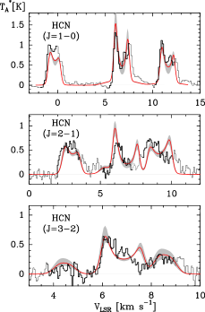
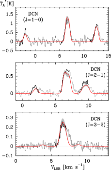
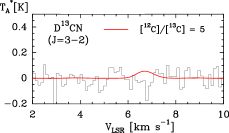
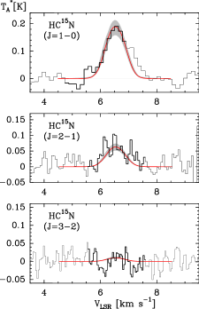
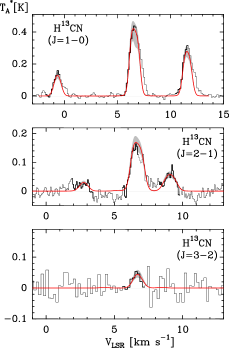
Figure 13: Observed (histograms) and modeled (red lines) spectra for (a) HCN ($J$=1-0) (top panel), HCN ($J$=2-1) (middle panel) and HCN ($J$=3-2) (bottom panel) (b) DCN ($J$=1-0) (top panel), DCN ($J$=2-1) (top panel) and DCN ($J$=3-2) (bottom panel) (c) D¹³CN ($J$ = 3-2) for a ratio of $\chi$(DCN) / $\chi$(D¹³CN) = 5 (red line) (d) HC¹⁵N ($J$=1-0) (top panel), HC¹⁵N ($J$=2-1) (middle panel) and HC¹⁵N ($J$=3-2) (bottom panel) (e) H¹³CN ($J$=1-0) (top panel), H¹³CN ($J$=2-1) (middle panel) and H¹³CN ($J$=3-2) (bottom panel) .

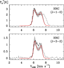
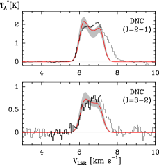
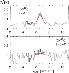
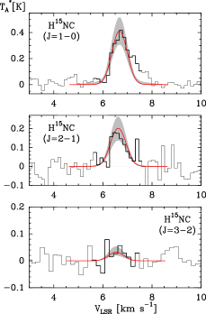
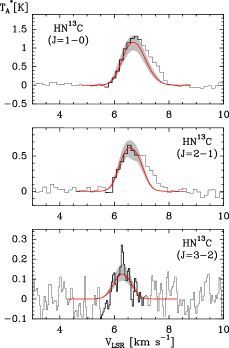
Figure 14: Observed (histograms) and modeled (red lines) spectra for (a) HNC ($J$=1-0) (top panel), and HNC (J=3-2) (bottom panel) (b) DNC ($J$=2-1) (top panel), and DNC ($J$=3-2) (bottom panel) (c) DN¹³C ($J$=2-1) (top panel), and DN¹³C ($J$=3-2) (bottom panel) (d) H¹⁵NC ($J$=1-0) (top panel), H¹⁵NC ($J$=2-1) (middle panel) and H¹⁵NC ($J$=3-2) (bottom panel) (e) HN¹³C ($J$=1-0) (top panel), HN¹³C ($J$=2-1) (middle panel) and HN¹³C ($J$=3-2) (bottom panel) .

The various isotopologues abundance profiles derived from the modeling is shown in Fig. 6 for HCN and in Fig. 7 for HNC. The comparison of the observations with the modeled line profiles are shown in Fig. 13 for the HCN isotopologues and in Fig. 14 for the HNC ones. In the case of D¹³CN, we could only derive an upper limit for the molecular abundance. The column densities for each isotopologue, as well as the column density ratios, are given in Table 2.

The current results show that the HCN/HNC column density ratio ranges from 2 to 4, depending on the isotopologue considered (omitting the D-substituted isotopologues). If we consider the ¹³C and ¹⁵N isotopologues, we obtain a mean ratio HCN/HNC $\sim$ 2.3. Additionally, we found that HCN shows the lowest degree of deuteration fractionation of all the molecules considered in this work and, in particular, the degree of deuteration is lower than for the HNC isomer. We thus obtained a ratio DCN/DNC $\sim$ 0.6. All of these findings are in good agreement with the predictions of chemical models (see e.g. Fig. 2 of Gerin et al., 2009).

A main uncertainty in the modeling of HCN and HNC comes from the fact that we obtained ¹²C/¹³C ratios which are respectively factors of 2 and 3 lower than expected for the local ISM (Lucas & Liszt, 1998). A main issue while modeling HCN is that the lines have large opacities. Indeed, as we can see in Table 2, the opacities we obtained for the $J$=1–0, 2–1 and 3–2 lines are $\sim$56, 90 and 37, respectively. With such high opacities, we can expect that part of the HCN molecules will be hidden since their emission will be subsequently absorbed by the outermost layers of the cloud.

In Fig. 15, we give the contribution of the various layers of the model to the emerging intensity, using the quantity:

$$I_{v}(x)=\int_{0}^{x}S_{v}(y)\,e^{-\tau_{v}(y)}\,dy$$ (4)

which gives the intensity at a velocity offset $v$, for an impact parameter which corresponds to the diameter of the cloud, $D$. The origin of the $y$–axis corresponds to the outer edge of the cloud where the photons escape. The integration from $y=0$ to $y=x$ thus indicates the number of photons created along that path and accounts for the subsequent absorption of the photons by the outermost layers and until the photons escape from the cloud at $y=0$. The emerging intensity is thus $I_{v}(D)$ and in Fig. 15, we show the quantity $(I_{v}(D)-I_{v}(x))/I_{v}(D)$, which indicates the percentage contribution of each radial point to the emerging intensity. In this figure, we show the contribution of the various regions to the emergent intensity, for the $J$=1–0 and $J$=3–2 lines and at various velocity offsets. When considering the abundance of HCN given in Fig. 6, we see that regions depleted in HCN, i.e. $0^{\prime\prime}<r<15^{\prime\prime}$ and to a lesser extent $50^{\prime\prime}<r<120^{\prime\prime}$, have no significant contribution to the emergent intensity. However, the whole region $15^{\prime\prime}<r<50^{\prime\prime}$ contributes to the line profile, and despite the large opacities, the innermost part of this region is still visible. The contribution at a given radius, however, depends on the frequency considered. For example, if we consider the velocity offset $v=0.07$ km s^-1 for the $J,F$=1,2–0,1 line, we see that 40% of the emergent flux is created in a thin layer, which is 1$\arcsec$ or 2$\arcsec$ wide, at a distance $r$$\sim$50$\arcsec$. When the velocity offset with respect to the hyperfine transition increases, the layer that contributes to the emergent flux becomes wider. This can be seen considering, for example, the velocity offsets $v=0.6$ km s^-1 for the $J,F$=1,2–0,1 line or $v=5.4$ km s^-1 for the $J,F$=1,1–0,1 line. Additionally, we can see that the contribution of the backward hemisphere is more important for the blue part of the spectra, while the red part is more significantly influenced by the front hemisphere. This effect, which can be seen considering the velocity offsets $v=-7.4$ km s^-1 and -6.6 km s^-1 for the $J,F$=1,0–0,1 line, is due to the infall motion we have introduced in the model. If we consider the relative contribution of various layers to the $J$=1–0 and $J$=3–2 lines, we can see that the region $120^{\prime\prime}<r<450^{\prime\prime}$ affects the $J$=1–0, line while the $J$=3–2 line remains mostly unaffected. The above conclusions are reached by considering a single impact parameter that crosses the center of the sphere. When comparing the models to the observations, various impact parameters have to be considered in order to perform the convolution with the telescope beam. However, the conclusions reached above remain true for other impact parameters. This explains why in Fig. 6, the abundance in every region has an upper boundary when we fully treat the coupling between the telescope beam and the emission that emerges from the cloud. Finally, given that all the regions where HCN is abundant contribute to some extent to the emerging profile, it is not possible, with the current model, to increase the HCN abundance in a given region without modifying the emerging intensity. Hence, with the current assumptions, it is impossible to increase the ¹²C/¹³C ratio to obtain a value that would be consistent with the local ISM value. To perform such a calculation, a multi–dimensional model would be needed.

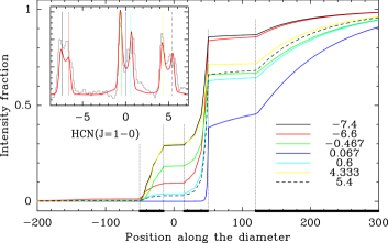
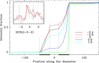
Figure 15: Contribution to the emergent HCN $J$=1–0 (upper panel) and 3–2 (lower panel) intensities by the different radii of the sphere, along the diameter. The dotted vertical lines indicate the radii $r=15\arcsec$, $50\arcsec$ and $120\arcsec$ that delimitate the regions where most of the photons are created. The main contribution to the emergent flux comes from the regions indicated by the bold segments in the $x$–axis. In each panel, the inset shows the emergent flux towards the centre of the model, and the vertical lines indicate the velocities for which we considered the propagation along the diameter of the sphere.

3.5 NH₃

3.5.1 spectroscopy and collisional rate coefficients

We used the collisional rate coefficients of Maret et al. (2009) which are calculated considering p–H₂($J$=0) as a collisional partner. For both NH₃ and ¹⁵NH₃, accurate rest frequencies for the hyperfine transitions have been measured by Kukolich (1967, 1968). The hamiltonian was subsequently refined by Hougen (1972). More recently, Coudert & Roueff (2009) determined a more extensive set of frequencies and line strengths using ab–initio calculations. These latter values are reported in the splatalogue database. In the NH₃ modelling, we used the values from Coudert & Roueff (2009), except for the (1,1) and (2,2) lines. For these lines, the spectroscopy was retrieved from the CLASS software since the rest frequencies are adapted from the experimental measurements and are of greater accuracy.

When computing excitation of ¹⁵NH₃, the RT is done including the unsplitted rotational levels of the molecule. The spectrum for the hyperfine structure is then obtained using the formula:

$$T_{A}^{hyp}(v)=\sum_{i}T_{A}^{rot}(v-v_{i})\times\frac{1-\textrm{exp}\left[-s_{i}\times\tau^{rot}(v-v_{i})\right]}{1-\textrm{exp}\left[-\tau^{rot}(v-v_{i})\right]}$$ (5)

where $T_{A}^{hyp}(v)$ is the antenna temperature of the hyperfine lines at a velocity offset $v$, $T_{A}^{rot}(v)$ the one of the rotational line, $v_{i}$ is the velocity offset of the $i^{th}$ hyperfine component, $s_{i}$ is its associated line strength and $\tau^{rot}(v)$ is the opacity of the rotational line. The rest frequencies and line strengths of the (1,1) line corresponds to the values given by Kukolich (1967, 1968).

3.5.2 Results

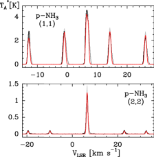
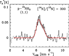
Figure 16: Observed (histograms) and modeled (red lines) spectra for (a) p–NH₃ (1,1) (top panel) and p–NH₃ (2,2) (bottom panel) (b) p–¹⁵NH₃ (1,1) .

Fig. 9 shows the isotopologue abundance profiles derived from the modeling. The comparison of the observations with the modeled line profiles is shown in Fig. 16. The column density for each isotopologue, as well as the column density ratios, are given in Table 2.

3.5.3 comparison with previous studies

The p–NH₃ emission toward B1b was studied by Bachiller et al. (1990); Rosolowsky et al. (2008); Johnstone et al. (2010); Lis et al. (2010). The current column density estimate, N(p–NH₃) = $5.5\,10^{14}$ cm^-2, is in reasonable agreement with the previous works. The p–NH₃ column density was estimated to $1.25\,10^{15}$ cm^-2 by Bachiller et al. (1990), $5.6\,10^{14}$ cm^-2 by Rosolowsky et al. (2008), $1.4\,10^{15}$ cm^-2 by Lis et al. (2010) and $6.5\,10^{14}$ cm^-2 by Johnstone et al. (2010). Note that except in the latter study, the authors reported the ortho+para NH₃ column density, with an ortho–to–para ratio of 1. The values reported here thus correspond to half of the column densities reported in these works. The column density estimates from the various studies agree within a factor $\sim$2, the current estimate being at the low–end of the reported values.

The NH₃ and ¹⁵NH₃ data used in the current study were previously analyzed by Lis et al. (2010). The column density ratio we obtained, i.e. N(NH₃)/N(¹⁵NH₃) = 300${}^{+55}_{-40}$ agree, within the error bars, with the previous estimate of 334${}^{+50}_{-50}$.

3.6 NH₂D

3.6.1 Collisional rate coefficients

For o–NH₂D, we used the collisional rate coefficients with He of Machin & Roueff (2006). Recently, rate coefficients for ND₂H with H₂ have been determined by Wiesenfeld et al. (2011) and it was shown that for this molecule, the rate coefficients with H₂ are, on the average, a factor 10 higher than the rate coefficients with He. We thus expect similar differences for NH₂D and, as a first guess, applied a scaling factor of 10 to the rate coefficients of Machin & Roueff (2006). However, with such an approach, the models fail to reproduce the spectral line shape of the $1_{1,1}s$–$1_{0,1}a$ line. In particular, in order to reproduce the overall intensities of the hyperfine lines, it is necessary to adopt an abundance that would produce a large opacity for this line (i.e. $\tau>10$). Subsequently, since the excitation temperature decreases with radius, this would entail that the main hyperfine component (i.e. $F$=2–2) would show a self–absorption feature which is not seen in the observed spectra. Consequently, in order to reproduce the observed profiles, it would be necessary to increase the density to decrease the opacity needed to fit the hyperfine multiplets.

Since all the other molecules are satisfactorily fitted with the current density profile, we examined in detail the impact of the assumption made on the collisional rate coefficients on the resulting line intensities. To do so, we used the Pearson’s correlation coefficient $r$ defined as :

$$r=\frac{\sigma_{xy}}{\sigma_{x}\,\sigma_{y}}$$ (6)

where $\sigma_{xy}$ is the covariance between variables $x$ and $y$, defined as :

$$\sigma_{xy}=\frac{1}{N}\sum_{i=1}^{N}\left(x_{i}-\bar{x}\right)\left(y_{i}-\bar{y}\right)$$ (7)

and $\sigma_{x}$ and $\sigma_{y}$ are the standard deviations with, for example :

$$\sigma_{x}=\sqrt{\frac{1}{N}\sum_{i=1}^{N}\left(x_{i}-\bar{x}\right)^{2}}$$ (8)

In the above expressions, $\bar{x}$ and $\bar{y}$ stand for the mean values of variables $x$ and $y$. The Pearson’s coefficient defines the correlation between two variables. The closest $|r|$ is to 1, the higher the correlation. When $r=0$, the two variables are independent.

As previously said, the ND₂H / He and ND₂H / H₂ rate coefficients differ, on the average, by a factor 10. But, when looking closely to the differences, it appears that there is a large scatter in the ratio, with values typically in the range 3–30. We thus performed RT calculations where we randomly multiplied the NH₂D / He rate coefficients by a factor in the range 5–20. The statistics is performed on a sample of 100 calculations. In order to assess the influence of a particular collisional rate coefficient on the resulting line intensity, we used the Pearson’s coefficient previously defined and we identified $x$ to be the integrated line intensity and $y$ the rate coefficient of a particular transition. The result of such a calculation is given in Figure 17.

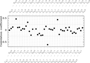
Figure 17: Correlation between the magnitude of the individual collisional rate coefficients for o–NH₂D with the integrated intensity of the $1_{1,1}s--1_{0,1}a$ line. For each transition, the Pearson’s correlation coefficient $r$ is given.

In this figure, it can be seen that most of the transitions have a correlation coefficient such that $|r|<0.25$. These transitions are thus only weakly correlated with the $1_{1,1}-1_{0,1}$ line intensity. Additionally, no transition appear to be strongly correlated with the line intensity, i.e. with $|r|\to 1$. This is due to the fact that since NH₂D is an asymmetric rotor, the pumping scheme is complex, which implies that the line intensity variations are due to various collisional transitions. The transitions that show the strongest correlation with the line intensity are the $1_{1,1}-1_{0,1}$, $2_{0,2}-1_{0,1}$, $2_{1,1}-1_{1,1}$ and $2_{2,1}-1_{0,1}$ transitions. Except for the $2_{1,1}-1_{1,1}$ transition, an increase of the rate coefficient is correlated with an increase of the line intensities. If we define a correlation coefficient that considers the sum of the rate coefficients for these transitions, weighted by $r/|r|$, we obtain a correlation coefficient $r=0.88$. This shows that most of the pumping scheme is related to these four transitions.

By comparing the rate coefficients for ND₂H with He and H₂, we can see that for the $1_{1,1}-1_{0,1}$, $2_{0,2}-1_{0,1}$, $2_{1,1}-1_{1,1}$ and $2_{2,1}-1_{0,1}$ transitions, the ratio are respectively $\sim$ 52, 12, 10 and 13 at 10K and $\sim$ 35, 10, 10 and 13 at 25K. We thus refine the scaling of the NH₂D / He rate coefficients, still applying an overall factor of 10 to the rates except for the $1_{1,1}-1_{0,1}$, $2_{0,2}-1_{0,1}$ and $2_{2,1}-1_{0,1}$ for which we apply factors of 45, 12 and 13, independently of the temperature. With rate coefficients defined in this way, we are able to reproduce more satisfactorily the o–NH₂D observations shown in Figure 18.

In order to test the influence of the above assumptions on the estimate of the NH₂D isotopologue column densities, we performed a few test calculations. More precisely, we ran models where the collisional rate coefficients of the various transitions were multiplied by a random factor between 1/1.5 and 1.5. From one set to the other, we found that the best models were obtained introducing variations in the $\chi$(NH₂D) radial distribution. These variations introduce changes in the column density estimates at most of the order of 50%. On the other hand, the changes in the column density ratios were found to be modest, always less than 10%, with respect to the value of N(NH₂D)/N(¹⁵NH₂D) = 230.

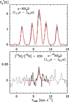
Figure 18: Observed (histograms) and modeled (red lines) spectra of o–NH₂D ($1_{1,1}s-1_{0,1}a$) (top panel) and o–¹⁵NH₂D ($1_{1,1}s-1_{0,1}a$) (bottom panel)

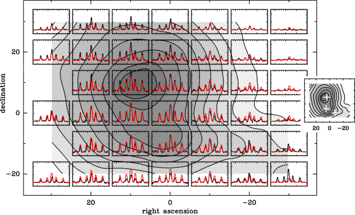
Figure 19: Map of the observed (histograms) and modeled (red lines) spectra of o–NH₂D ($1_{1,1}s-1_{0,1}a$). The background correspond to a map of the iscocontours of the intensity integrated of all the hyperfine components. The map on the right–hand side shows the isocontours with the same scale for the right ascension and declination. The white crosses indicate the position of the B1-bN and B1-bS sources identified by Hirano et al. (1999), as well as the Spitzer source reported by Jørgensen et al. (2006).

3.6.2 Results

The isotopologue abundance profiles derived from the modeling are shown in Fig. 9. The comparison of the observations with the modeled line profiles are shown in Fig. 18 for both isotopologues and in Fig. 19 we compare the $1_{11}-1_{01}$ NH₂D map with the model.

3.6.3 Comparison with previous studies

The NH₂D and ¹⁵NH₂D observations considered in this work were previously analyzed by Gerin et al. (2009). In that study, the column densities for both isotopologues were retrieved using LTE, which assumes a uniform distribution for the energy levels throughout the source and the respective populations of the upper and lower energy levels given by the excitation temperature T_ex. Since NH₂D has hyperfine components resolved in frequency, it is possible to obtain an estimate of both the excitation temperature and the total opacity of the rotational line. These parameters were retrieved using the hyperfine method of CLASS. The values obtained were T_ex = 6K and $\tau$ = 5.24 which agree within $\sim$20% with the averaged values T_ex = 6.5K and $\tau$ = 6.4 derived in the present work. Using, e.g., Eq. (1) of Lis et al. (2002), both sets of values lead to column density estimates that agree within 15%. On the other hand, the hyperfine components of ¹⁵NH₂D are not resolved and using this methodology, it is not possible to estimate both T_ex and $\tau$ from the observations. It was thus assumed that the excitation temperature of ¹⁵NH₂D is equal to that of NH₂D, which then enables to estimate the opacity of the line from the observed spectra. However, within the current methodology, we obtain an excitation temperature for ¹⁵NH₂D which is 30% lower than that of NH₂D, which is a consequence of larger line trapping effects for the more opaque isotopologue. This difference in the value of the excitation temperature for ¹⁵NH₂D is important when estimating the line opacity. As an example, using T_ex = 5K rather than the value of 6K used in Gerin et al. (2009), leads to an increase of the line opacity by a factor of 1.5. This subsequently leads to reestimate the ¹⁵NH₂D column density which is increased by a factor of 2. By examining Eq. (1) of Lis et al. (2002), we can see that the strong dependence of the column density on the excitation temperature comes from the term $\textrm{exp}(E_{u}/k_{b}\,T_{ex})$, and is due to the fact that the excitation temperature of the $1_{11}--1_{01}$ transition is low by comparison with the energy of the upper level ($E_{u}\sim 20.7$ K). This strong dependence of the ¹⁵NH₂D column density on the excitation temperature explains why the ¹⁴N/¹⁵N column density ratio was estimated to be $470^{+170}_{-100}$ in Gerin et al. (2009), while the current estimate is $230^{+105}_{-55}$.

The o–NH₂D map in Fig. 19 shows the peak intensity close to the B1–bN core. The emission is elongated towards the position of B1–bS, but the line intensities are lower towards this position. It was found by Huang & Hirano (2013), while discussing the deuterium fractionation of N₂H⁺, that the deuterium enrichment is a factor of two higher towards the B1–bN position compared to B1–bS. The current NH₂D observations suggest a similar trend for this species. The fit of the SED performed by Hirano et al. (2013) suggests that B1–bS has a temperature higher by a few Kelvins compared to B1–bN, with a temperature close to 20K for the former source. The lower level of deuterium enrichment towards B1–bS could thus be related to the fact that the temperature of the dust is close to the temperature at which CO desorbs. A higher amount of CO in the gas phase would drastically reduce the amount deuterated isotopologues of H${}_{3}^{+}$ and would thus limit the deuteration fraction.

3.7 CN

3.7.1 Spectroscopy and collisional rate coefficients

Since CN is an open shell molecule, its rotational energy levels are split into fine structure levels due to the interaction with the electron spin. These levels are further split because of the interaction with the nuclear spin of the nitrogen atom. In the case of the ¹³CN and C¹⁵N isotopologues, the 1/2 spins of the ¹³C and ¹⁵N nuclei lead to magnetic coupling, which have associated coupling constants sufficiently large, so that the degeneracy break can be spectroscopically resolved.

For CN, we have used the CN / He collisional rate coefficients of Lique & Kłos (2011). For either ¹³CN or C¹⁵N, the energy pattern is modified compared to CN, because of the large magnetic coupling constants associated with the ¹³C or ¹⁵N nuclei. Since all these molecules have specific energy structures, it is not possible to directly use the CN / He collisional rate coefficients to obtain the ¹³CN or C¹⁵N rates. Hence, in the present study, we derived the rate coefficients for the rarest isotopologues from the diffusion matrix elements obtained for the CN / He system but accounting for their specificities, while performing the recoupling of the matrix elements. The description is given in the Appendix and these rates will be made available through the BASECOL database (Dubernet et al., 2013).

In the case of CN, rate coefficients for the CN / p–H₂ system have recently been calculated by Kalugina et al. (2012). They show that individual state–to–state rate coefficients with He or H₂ can differ by up to a factor 3. However, these differences mainly affect the rates of lowest magnitude, while the highest ones scale accordingly to the factor expected from the differences in the reduced masses of the two collisional systems. For consistency between the various isotopologues, we used the CN / He collisional rate coefficients of Lique & Kłos (2011) for the main isotopologue.

3.7.2 Results

The various isotopologue abundance profiles derived from the modeling are shown in Fig. 8. In Fig. 20 we compare the model with the observations of the $N$=1–0 and $N$=2–1 spectra of CN and ¹³CN and of the $N$=1–0 transition of C¹⁵N. Note that in the $N$=1–0 CN spectrum, a transition due to the doubly deuterated thioformaldehyde isotopologue is seen at a velocity offset $v\sim$22 km s^-1 (Marcelino et al., 2005). The column densities for each isotopologue, as well as the column density ratios, are given in Table 2. In this study, we report the first observations made for the various CN isotopologues toward B1b.

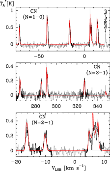
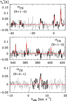
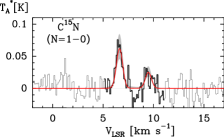
Figure 20: Observed (histograms) and modeled (red lines) spectra for (a) CN ($N$=1–0) (top panel), and CN ($N$=2–1) (middle and bottom panel) (b) ¹³CN ($N$=1–0) (top and middle panel), and ¹³CN ($N$=2–1) (bottom panel) (c) C¹⁵N ($N$=1–0) .

4 Discussion

In the upper panel of Fig. 21, we report the abundance profiles of the main isotopologues as a function of the H₂ density. These abundances are obtained from a polynomial fit to the discrete values reported in Fig. 5-9, where all the regions of the model, except the region with $r>120^{\prime\prime}$ are considered. In Figures 5 to 9, it can be seen that the molecular abundances have large errorbars when the abundance is much below the maximum abundance found for a given molecule. This means that in Fig. 21, we expect the abundances to be accurate within a factor of a few around $10^{5}$ cm^-3, while around $10^{4}$ cm^-3 and $10^{6}$ cm^-3, the error will be typically of an order of magnitude. This can be seen in the middle and bottom panel of Fig. 21 where the abundances used in the fit, as well as their estimated error bars, are reported for the hydrogenated and deuterated isotopologues of NH₃ and N₂H⁺. The abundances reported in this figure can be directly compared to the prediction of the gas–phase chemical model in Fig. 2 of Gerin et al. (2009). While the molecular abundances inferred from the observations agree with the predictions of this chemical model at low densities, the current modeling shows that all the molecules are expected to suffer depletion at densities above $10^{5}$ cm^-3 and are then considerably lower than predicted by the gas–phase chemistry.

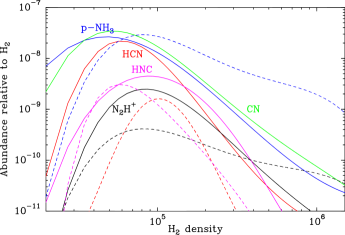
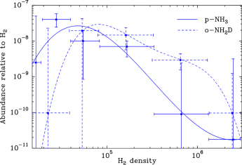
Figure 21: Abundances of the various molecules observed in this study as a function of the H₂ density (upper panel). The full lines show the abundances of the main species and the dashed lines the abundances of the deuterated isotopologues. The abundances are obtained by fitting the step functions used in the RT modelling. The central and bottom panels give the initial points used in the fit as well as the error bars for NH₃ and N₂H⁺.

4.1 Molecular depletion and consequences on the N₂H⁺ and NH₃ excitation

Johnstone et al. (2010) re–analyzed the N₂H⁺ and 850 $\mu$m continuum observations of Kirk et al. (2007) by combining them with the p–NH₃ observations of Rosolowsky et al. (2008), for a number of prestellar and protostellar objects in the Perseus molecular cloud. They found that the column density ratio of these two species is relatively constant regardless of the evolutionnary stage of the object, with N(p–NH₃)/N(N₂H⁺) = 22 $\pm$ 10. Our results for the B1b region, i.e. N(p–NH₃)/N(N₂H⁺) = 18, are thus in good agreement with the earlier results. Additionally, Johnstone et al. (2010) found that the p–NH₃ abundance is rather constant in all the prestellar cores, i.e. $\chi$(p–NH₃) $\sim$ 10^-8, while there is a larger scatter for the protostellar objects, where it ranges from 10^-8 at low H₂ column densities and decreases by an order of magnitude at larger column densities.

Johnstone et al. (2010) also derived a tight correlation between the excitation temperatures of the N₂H⁺ ($J$=1–0) and p–NH₃ (1,1) transitions, with a tendency for the p–NH₃ excitation temperature to be higher by 1K. Their sample is consistent with constant excitation temperatures, independently of the central density of the objects. Again, our current results for the B1b region, reported in Table 2, i.e. T_ex(N₂H⁺) $\sim$ 6.8 K and T_ex(p–NH3) $\sim$ 8.1 K, confirm the tendency outlined by Johnstone et al. (2010). As pointed out by these authors, the similarity of the excitation temperatures for these two species is puzzling when considering the critical densities of the respective transitions. More precisely, the excitation temperatures are below the estimated kinetic temperatures of the studied regions which indicates subthermal excitation. Indeed, Johnstone et al. (2010) found that the dust emission at 850 $\mu$m can be reproduced assuming T_d $\sim$ 11K. For densities higher than $10^{4}$ cm^-3, the kinetic temperature is believed to be well coupled to the dust temperature (Goldsmith, 2001). However, considering the differences in the critical densities, the p–NH₃ excitation temperature should be higher than that of N₂H⁺, if the molecules trace the same volume of gas. As pointed out by these authors, similar excitation temperatures would require densities large enough for the lines to be thermalized. Hence, they stress that the excitation temperatures for both species may have been underestimated. Our current results shed some light on the puzzling behaviour reported by Johnstone et al. (2010). Indeed, considering the spatial distribution of $\chi$(p–NH₃) and $\chi$(N₂H⁺) shown in Fig. 5 and 9, we see that N₂H⁺ has an abundance distribution more centrally peaked than p–NH₃. Since the innermost region of the cloud is warmer and denser, this enhances the mean excitation temperature of N₂H⁺ with respect to that of p–NH₃, thus reducing the impact of the differing critical densities. Moreover, our models show that both molecules are removed from the gas phase in the innermost part of the cloud. If we consider that both molecules suffer depletion above a given density, it entails that the properties derived from both molecules will characterize the gas which is below this density threshold. On the other hand, the dust will still trace the total volume of gas. Thus, if depletion affects both p–NH₃ and N₂H⁺, it can explain why Johnstone et al. (2010) conclude that the p–NH₃ and N₂H⁺ excitation temperatures are independent of the central H₂ density.

Tobin et al. (2011) presented interferometric observations of NH₃ and N₂H⁺ in a sample of class 0 and class I protostars. In particular, they observed that the position of the maximum intensity in these two tracers was offset from the position of the continuum peak, hence from the position of the protostar. Apart from depletion, an alternative way to explain the disappearance of these molecules from the gas phase can be chemical destruction. Above 20K, CO will be released from the ice mantles and will react with N₂H⁺ to form HCO⁺. Hence, this reaction will efficiently destroy N₂H⁺. Such a process has been invoked by Tobin et al. (2013) in order to explain the central hole observed for both the N₂H⁺ and N₂D⁺ abundances in the protostellar object L1157. Additionally, in this object, N₂H⁺ is found to be more centrally peaked than N₂D⁺, which might be a consequence of variations in the H₂ ortho–to–para ratio. In the case of NH₃, an efficient destruction can come from the reaction with HCO⁺ (Woon & Herbst, 2009). Thus, chemical destruction could explain the shape of the abundance profiles we obtain for NH₃ and N₂H⁺ in the B1b region. Two arguments can be invoked against such an possibility. First, the observations of H¹³CO⁺ performed by Hirano et al. (1999) showed that at the positions of B1-bS and B1-bN, the abundance of this molecule was reduced by a factor of the order $\sim$ 3-5 with respect to the H¹³CO⁺ abundance of the surrounding envelope. Second, the dust temperature obtained from the SED fitting is found to be below 20K. Hence, the hypothesis of depletion seems to be favored in order to explain the central decrease in the N₂H⁺ and NH₃ abundances.

The fact that NH₃ is strongly depleted onto dust grains in the innermost region of B1b is strengthened by the analysis of the NH₃ ice features. At the position of the Spitzer source which is offset by $\sim$15$\arcsec$ from the central position of our model, Bottinelli et al. (2010) inferred a total column density of NH₃ locked in the ice of $\sim$$7\,10^{17}$ cm^-2, while we derive a column density N(p–NH₃) $\sim$$5.5\,10^{14}$ cm^-2 in the gas phase, at the central position of our observations. Converting this column density to the total amount of NH₃ requires knowledge of the respective abundances of ortho– and para–NH₃. It is expected that if NH₃ is formed in the gas phase, the ratio will be of the order of unity. On the other hand, a formation that would occur on dust grains would raise the ortho–to–para ratio above unity (Umemoto et al., 1999). If we assume a similar amount of ortho and para–NH₃, this leads to a total gas phase column density of N(NH₃) $\sim 1\,10^{15}$ cm^-2. Since the observations of Bottinelli et al. (2010) are offset with respect to our core center, we can infer that the gas phase NH₃ abundance is a factor $>$$700$ lower than inferred from the ice feature observations.

In principle, the comparison of the respective abundances in the gas and solid phases should shed light on the evolutionary stage of the source. Indeed, it is predicted theoretically that the relative abundance of NH₃ in both phases will vary with time during the collapse (e.g. Rodgers & Charnley, 2003; Lee et al., 2004; Aikawa et al., 2008, 2012). In particular, after the formation of a protostar, the NH₃ molecules locked in the ices will be released into the gas phase, because of the warm–up, and the ratio of the NH₃ gas–to–dust abundances will increase with time. However, in the present case, this point can only be discussed qualitatively, because of the simplicity of the geometry we assumed to describe the B1b region. We consider a 1D–spherical model while two objects, B1–bS and B1-bN are present and separated by a projected distance of only $\sim$20$\arcsec$. Moreover, if we consider e.g. Fig. 2 of Aikawa et al. (2012), we see that $\sim$500 years after the formation of a protostar, the increase of the NH₃ abundance in the gas phase occurs at the 10 AU scale (i.e. $\sim$0.04$\arcsec$ at 235 pc), and at the 100 AU scale at $t=10^{4}$ years. This makes the FHSC stage ($t$ = -560 yr in Aikawa et al. (2012) where $t=0$ corresponds to the formation of the second hydrostatic core, i.e. the protostar) hardly distinguishable from the stage that harbours a newly born protostar, at least in single dish observations. Thus, the abundance profile we derived for the gas–phase p–NH₃ abundance would be consistent with the predictions of Aikawa et al. (2012) from $t=-560$ yr to $t=10^{4}$ yr and it is thus impossible to infer from these observations the evolutionary stage of the two sources in the B1b region, i.e. to disentangle the FHSC stage from the class 0 stage.

4.2 Deuteration

The abundance profiles reported in Fig. 21 show that at the innermost radii, the behaviour of the p–NH₃ and o–NH₂D abundances changes, with a ratio $\chi$(o–NH₂D) / $\chi$(p–NH₃) below unity for densities lower than $\sim 6\,10^{4}$ cm^-3, and above unity for higher densities. We found that this enhancement is higher than an order of magnitude at the core center. Hence, this behaviour will still be true if we consider the total column densities of NH₃ and NH₂D and if we consider standard ratios to relate the abundances of the ortho and para species. Fig. 3 of Aikawa et al. (2012) shows that a ratio $\chi$(NH₂D)/$\chi$(NH₃) $>1$ is expected at small radii, but only at an evolutionary stage close to the FHSC stage. At times greater than 500 yrs after the formation of the first hydrostatic core, the NH₃ abundance always exceeds the NH₂D abundance throughout the envelope. This is due to the fact that when the gas temperature becomes high enough, the backward reaction that leads to the deuterated isotopologues of H${}_{3}^{+}$ becomes efficient enough to inhibit the deuteration of this ion. Finally, the NH₂D map in Fig. 19 shows that the NH₂D peak is close to the position of the B1–bN core. This would suggest that this core is closer to the FHSC stage than B1–bS.

4.3 Nitrogen fractionation

To date, there have been few studies estimating the abundance ratio of ¹⁴N and ¹⁵N isotopologues in dark clouds. In the source L1544, the ¹⁴N/¹⁵N ratio was estimated to be $1000\pm 200$ by Bizzocchi et al. (2010, 2013) for the N₂H⁺ isotopologues. Toward the same source, Hily-Blant et al. (2013) estimated $140<$ ¹⁴N/¹⁵N $<360$ for the HCN molecule, using a double–isotope analysis of H¹³CN and HC¹⁵N. In the same study, a similar analysis was also performed towards L183 leading to $140<$ ¹⁴N/¹⁵N $<250$. Ikeda et al. (2002) observed HCN and CO isotopologues in a sample of three dark clouds in the Taurus molecular cloud. They derived values of $151\pm 16$ and $>813$ for L1521E and L1498 respectively using the ¹²C/¹³C ratio derived from the analysis of the CO isotopologues. In the case of L1498, this ratio was determined to be ¹²C/¹³C$>117$ from the analysis of ¹³C¹⁸O and ¹²C¹⁸O lines, a value significantly higher than the standard value in the local ISM. Assuming a ratio of 60 rather than 117 would lead to HCN / HC¹⁵N = $472\pm 55$. Moreover, both Ikeda et al. (2002) and Hily-Blant et al. (2013) found that the H¹³CN/HC¹⁵N abundance ratio varies as a function position. As pointed out by Ikeda et al. (2002), this result can be interpreted either as due to an incomplete mixing of the parental gas, or variations in the chemistry of nitrogen fractionation within the clouds.

The NH₃ and NH₂D data considered in the present study were already analyzed by Lis et al. (2010) and Gerin et al. (2009), using a LTE approach. In the case of NH₃, the isotopologue abundance ratio was found to be $334\pm 50$, in good agreement with the present determination of $300^{+55}_{-40}$. However, in the case of NH₂D, we obtain a value of $230^{+105}_{-55}$ compared to the earlier estimate of $470^{+170}_{-100}$. As explained in Sect. 3.6, this comes from the fact that the assumption of equal excitation temperatures for NH₂D and ¹⁵NH₂D made in Gerin et al. (2009) is not totally valid. Moreover, we found that variations as small as $\sim$20% in the excitation temperatures lead a factor 2 variations in the column density ratio. Apart from B1b, Lis et al. (2010) and Gerin et al. (2009) reported column density ratio estimates in other dark clouds. A value of $344\pm 173$ was obtained for NH₃ in NGC1333 and for NH₂D, values in the range 350 $<$ ¹⁴N/¹⁵N $<$ 850 were obtained in a sample of four clouds. In the latter case, as for B1b, the column density ratio may have been overestimated by a factor $\sim$2.

Tennekes et al. (2006) reported observations of various HCN and HNC isotopologues towards Cha–MMS1. They analyzed the emission from these molecules both with a non–LTE non–local radiative transfer modelling and with the LTE approach. In their non–LTE analysis, they fixed the isotopologue abundances assuming ¹²C/¹³C = 20 and ¹⁴N/¹⁵N = 280, on the base of their LTE analysis. At that time, it was not yet recognized that the HCN and HNC collisional rate coefficients could differ by a significant factor. Indeed, in their LTE analysis, they assumed a single excitation temperature for all the HCN and HNC isotopologues. However, due to differing HCN and HNC rate coefficients and because of line trapping effects that affect the main isotopologues, this assumption is not valid as can be seen in Table 2.

An estimate of the ¹⁴N/¹⁵N galactic gradient was reported by Dahmen et al. (1995) from HCN observations and Adande & Ziurys (2012) from CN and HNC observations. The first study used a double isotope method with a ¹²C/¹³C ratio based on H₂CO observations. However, H₂CO might undergo carbon fractionation effects and the results from Dahmen et al. (1995) were then reanalyzed by Adande & Ziurys (2012) assuming a different ¹²C/¹³C ratio as derived from the CN observations of Milam et al. (2005). From both HCN, HNC and CN, they obtain a value for the local ISM of ¹⁴N/¹⁵N = $290\pm 40$. The sample of clouds used in these studies have typical kinetic temperatures in the range 25K $<$ T_K $<$ 90K (Adande & Ziurys, 2012). At such high kinetic temperatures, fractionation effects for the nitrogen are unlikely to occur and the value quoted should thus be representative of the elemental atomic abundance ratio. This estimate is in good agreement with the estimate of ¹⁴N/¹⁵N = 237${}_{-21}^{+27}$ obtained toward diffuse clouds of the local ISM observed in absorption toward compact extragalactic sources (Lucas & Liszt, 1998).

The values obtained in the current study for the column density ratios are summarized in Fig. 22. In this figure, we also report the mean ratio ($\sim$296) computed from all the values except that of ¹⁵NNH⁺, for which we only obtained a lower limit. In the figure, for this molecule, we indicate this lower limit as well as approximate error bars which are obtained by scaling that of N¹⁵NH⁺. The values reported for the nitriles come from the double isotope method rather than from a direct estimate (see Sect. 3.4). By examining Fig. 22, it can be seen that given the errorbars, the column density ratios are consistent with a constant value. The only exception is N₂H⁺, and particularly ¹⁵NNH⁺, for which a higher ¹⁴N/¹⁵N ratio is obtained. The current result support the conclusion that no fractionation affects the nitrogen chemistry in the B1b region. The mean value we obtain for B1b is in good agreement with the estimate of $290\pm 40$ (Adande & Ziurys, 2012) obtained toward warmer sources in the local ISM. This latter value could be representative of the gas associated with the Perseus molecular cloud. But, it was also recognized (Ikeda et al., 2002; Adande & Ziurys, 2012) that the elemental ¹⁴N/¹⁵N atomic ratio can vary from source to source. The absence of large differences between the nitriles and the nitrogen hydrides obtained in the current study suggest that no fractionation effects occur in B1b and a ratio ¹⁴N/¹⁵N $\sim$ 300 should thus be representative of this region.

However, two things must be kept in mind while considering this conclusion. The first point is that the N₂H⁺ column density ratio show a tendency towards higher values, in particular for ¹⁵NNH⁺, for which we derived a lower limit N(N₂H⁺) / N(¹⁵NNH⁺) $>$ 600. The second point concerns the nitriles. For this family, we derived the main isotopologue column densities from the ¹³C isotopologues assuming a ratio ¹²C/¹³C = 60. This value is representative of the local ISM, but as for the nitrogen case, can be affected by source–to–source variations.

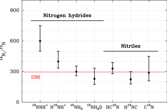
Figure 22: ¹⁴N/¹⁵N isotopologue abundance ratio for the molecules of the nitrogen hydride and nitrile families.

The astrochemical modelling by Wirström et al. (2012) suggests that the nitrogen hydride and nitrile families should show different degrees of fractionation. Such a finding is supported by the results of Ikeda et al. (2002) and Hily-Blant et al. (2013) where low ¹⁴N/¹⁵N ratios were derived for HCN. Such differential fractionation effects are appealing since they would enable to reconcile some of the observations made in the solar system. However, in the current study, no differential fractionation is found between the nitrogen hydride and nitrile families. Regarding the absence of fractionation in B1b, a possible explanation may be that this region contains two cores in a late evolutionary stage. The gas temperature in the core center is estimated to be $\sim$17K, somewhat higher than the lowest temperatures $\sim$7K that can be reached during the prestellar phase. Similarly to our definition of the mean excitation temperature given in Sect. 3.2, we can define a mean gas temperature, averaged over all the molecules considered in this work, that describes the mean temperature of the gas from which the emission originates. We find that $\overline{T}_{K}=13.7^{+1.9}_{-2.6}$ K. At such high temperatures, the nitrogen fractionation might already be ineffective. Indeed, as shown by Rodgers & Charnley (2008), decreasing the gas temperature from 10K to 7K can lead to an increase by a factor $\sim$3 in the ¹⁵N–enrichment for the NH₃ and N₂ molecules. This effect is partly due to the low exothermicity of the exchange reactions that involve the ¹⁵N⁺ ions, which are typically in the range $\Delta E=20-30$K. As a consequence, small variations of the temperature around the canonical value of 10K, commonly used to describe prestellar cores, could result in substantial variations in ¹⁵N–fractionation effects, because of the variations of the backward reaction rates. However, to date, a quantitative estimate of the amount of ¹⁵N–fractionation for temperatures higher than 10K has never been addressed by astrochemical models. The strong dependence of ¹⁵N–fractionation effects with temperature would imply that the ¹⁴N/¹⁵N ratio should vary within the sources with temperature gradients. However, this issue cannot be addressed in the present study, since to test this hypothesis it would be necessary to constrain the models on the basis of emission maps of the ¹⁵N–substituted species. Finally, the current model shows that at the core center, all the molecules are affected by depletion onto dust grains. Thus, it cannot be discarded that fractionation effects could have occurred earlier in the life of the B1b cloud. However, the ¹⁵N enrichment would nowadays be unobservable, since the molecules formed in the previous colder evolutionary stages would have been subsequently incorporated into the ice mantles that surround the dust grains.

As discussed by Wirström et al. (2012), in order to link the prestellar phase chemistry with the observations of the solar system, the astrochemical models have to be able to produce high degrees of fractionation for both ¹⁵N and D substituted isotopologues. Another prerequisite is that they also have to account for the fact that the meteoritic hot–spots for these two isotopes are not necessarily coexistents. In the present case, while no ¹⁵N–fractionation is seen for both the nitriles and nitrogen hydrides in B1b, we conclude that the nitrogen hydrides are highly fractioned in deuterium. The D–fractionation for the nitriles is also found to be high, even if lower than for the nitrogen hydride family. Hence, the gas depleted at this evolutionary stage will create hot–spots in D and will not be associated with high ¹⁵N enrichments.

5 Conclusion

We report a model based on continuum emission and molecular line observations for the B1b region, located in the Perseus molecular cloud. First, we modelled the 350 $\mu$m and 1.2 mm continuum radial profiles to obtain an estimate of the temperature and H₂ density distributions in the source. These density and temperature profiles were subsequently used as an input for the non–local radiative transfer modeling of the molecular lines. The molecular data include D–, ¹³C– and ¹⁵N–substituted isotopologues of molecules that belong to the nitrogen hydride family, i.e. N₂H⁺ and NH₃, as well as molecules from the nitrile family, i.e. HCN, HNC and CN. For each molecule, the radial abundance profile was divided in several zones, in which the molecular abundance was considered as a free parameter. The best estimate for the abundance profile was then obtained from a Levenberg–Marquardt algorithm, which minimizes the $\chi^{2}$ between models and observations. Additionally, since our ¹³C– and ¹⁵N– observations are only towards a single position, we assumed that the various isotopologues have abundance profiles that only differ by a scaling factor.

A common feature obtained for all the molecules is that in the innermost part of B1b, all the molecules have abundances, which are at least one order of magnitude lower than the peak abundance found in the envelope. Since all the molecules seem affected, this feature is interpreted as depletion onto dust grains rather than due to chemical destruction, a process that might be invoked for N₂H⁺ since the innermost region of B1b has a temperature which is close to the CO thermal desorption temperature. We derived high degrees of deuteration with the D/H ratio increasing inwards. On the other hand, we derived similar ¹⁴N/¹⁵N abundance ratios for all the molecules and independently of the chemical family, with an average ratio of $\sim$300. This value is consistent with a recent estimate of the ¹⁴N/¹⁵N atomic elemental abundance ratio obtained for warmer sources in local ISM. We thus conclude that the ratio ¹⁴N/¹⁵N$\sim$300 inferred from the molecules is representative of the atomic elemental abundances of the parental molecular cloud. We propose that the absence of ¹⁵N–fractionation in B1b is a consequence of the relatively high gas temperature of this region, as compared to the low temperatures that can be reached during the prestellar phase. The current state of the chemistry in B1b would not produce any ¹⁵N–fractionation. On the other hand, it cannot be excluded by the current observations that conditions favorable to produce a ¹⁵N–enrichment were met during earlier evolutionary stages of the cloud. Since the molecules are found to be affected by depletion onto dust grains, the products of such a chemistry could have been incorporated into the ice mantles that surround the dust grains.

Given that ¹⁵N–fractionation effects can have strong implications for our understanding of the diversity observed in the various bodies of the solar system, it would be important to extend such a study focusing on earlier evolutionary stages with lower gas temperature, more favorable for producing nitrogen fractionation. Additionally, it was found in the current study that a direct estimate of the fractionation in the nitriles, i.e. HCN and HNC, is difficult because of the large opacities of the lines. This difficulty is not found for CN since this molecule is an open–shell molecule, which leads to a redistribution of the total opacity of the rotational line over a larger number of radiative transitions. Observations of less abundant species from this family, like HC₃N, would thus be particularly helpful. Moreover, we had to use the double isotope method to estimate the HCN and HNC column densities, from the H¹³CN and HN¹³C isotopologues. We assumed the standard ¹²C/¹³C elemental ratio, which introduces uncertainties due to possible source–to–source variations. It would thus be helpful to complement the set of molecular observations with other carbon bearing molecules, like e.g. C¹⁸O.

Finally, we have shown that the isotopic ratios are sensitive to the assumptions made in deriving the column densities. Even relatively small differences in excitation temperatures of different isotopologues may lead to large variations in the derived isotopic ratios. The use of a sophisticated radiative transfer method is therefore recommended.

Appendix A Inelastic rate coefficients for the CN isotopologues

We used the two dimensional CN–He PES of Lique et al. (2010) to determine hyperfine resolved excitation and de-excitation cross sections and rate coefficients of C¹⁵N and ¹³CN molecules by He. CN–He rate coefficients obtained from this PES were found to be in excellent agreement with the experimental rotational (with unresolved fine and hyperfine structure) rate coefficients of Fei et al. (1994) . This agreement demonstrate the accuracy of the PES and suggests that the rate coefficients obtained from this potential will be accurate enough to allow for improved astrophysical modeling of the ISM.

The Alexander’s description (Alexander, 1982) of the inelastic scattering between an atom and a diatomic molecule in a ${}^{2}\Sigma^{+}$ electronic state and a fully-quantum close-coupling calculations was used in order to obtain the $S^{J}(jl;j^{\prime}l^{\prime})$ diffusion matrix between fine structure levels of CN. $J$ and $l$ denote the total angular momentum ($\@vec{J}=\@vec{j}+\@vec{l}$) and the orbital angular momentum quantum numbers, respectively. The nuclear spin-free $S^{J}(jl;j^{\prime}l^{\prime})$ matrix were computed recently in Lique & Kłos (2011) and we used these matrices in the following.

For C¹⁵N, The coupling between the nuclear spin ($I=1/2$) of the ¹⁵N atom and the molecular rotation results in a weak splitting (Alexander & Dagdigian, 1985) of each rotational level $j$. Each hyperfine level is designated by a quantum number $F$ ($F=I+j$) varying between $|I-j|$ and $I+j$. The integral cross sections corresponding to transitions between hyperfine levels of the C¹⁵N molecule can be obtained from scattering S-matrix between fine structure levels using the re-coupling method of Alexander & Dagdigian (1985). Inelastic cross sections associated with a transition from the initial hyperfine level ($NjF$) to a final hyperfine level ($N^{\prime}j^{\prime}F^{\prime}$) were thus obtained as follow :

$$\sigma_{NjF\to N^{\prime}j^{\prime}F^{\prime}} = \frac{\pi}{k^{2}_{NjF}}(2F^{\prime}+1)\sum_{K}$$ (11)

$$\times\left\{\begin{array}[]{ccc}j&j^{\prime}&K\\ F^{\prime}&F&I\end{array}\right\}^{2}P^{K}(j\to j^{\prime})$$

The $P^{K}(j\to j^{\prime})$ are the tensor opacities defined by :

$$P^{K}(j\to j^{\prime})=\frac{1}{2K+1}\sum_{ll^{\prime}}|T^{K}(jl;j^{\prime}l^{\prime})|^{2}$$ (12)

The reduced T-matrix elements (where $T=1-S$) are defined by Alexander & Davis (1983):

$$T^{K}(jl;j^{\prime}l^{\prime}) = (-1)^{-j-l^{\prime}}(2K+1)\sum_{J}(-1)^{J}(2J+1)$$ (15)

$$\times\left\{\begin{array}[]{ccc}l^{\prime}&j^{\prime}&J\\ j&l&K\end{array}\right\}T^{J}(jl;j^{\prime}l^{\prime})$$

For ¹³CN, the situation is more complex since both the ¹³C and N atoms have non zero nuclear spin. The coupling between the nuclear spin ($I_{1}=1/2$) of the ¹³C atom and the molecular rotation is first taken into account. Each hyperfine level is designated by a quantum number $F_{1}$ ($F-1=I_{1}+j$) varying between $|I_{1}-j|$ and $I_{1}+j$. The coupling between the nuclear spin ($I_{2}=1$) of the N atom and the first hyperfine state is then taken into account. Each hyperfine level is designated by a quantum number $F$ ($F=I_{2}+F_{1}$) varying between $|I_{2}-F_{1}|$ and $I_{2}+F_{1}$. The integral cross sections corresponding to transitions between hyperfine levels of the ¹³CN molecule can be obtained from scattering S-matrix between fine structure levels also using the re-coupling method of Alexander & Dagdigian (1985). Inelastic cross sections associated with a transition from the initial hyperfine level ($NjF_{1}F$) to a final hyperfine level ($N^{\prime}j^{\prime}F_{1}^{\prime}F^{\prime}$) were thus obtained as follow (Daniel et al., 2004):

$$\sigma_{NjF_{1}F\to N^{\prime}j^{\prime}F_{1}^{\prime}F^{\prime}}=\frac{\pi}{k^{2}_{NjF}}(2F_{1}+1)(2F_{1}^{\prime}+1)(2F^{\prime}+1)$$

$$\times\sum_{K}\left\{\begin{array}[]{ccc}F_{1}&F_{1}^{\prime}&K\\ F^{\prime}&F&I_{2}\end{array}\right\}^{2}\left\{\begin{array}[]{ccc}j&j^{\prime}&K\\ F_{1}^{\prime}&F_{1}&I_{1}\end{array}\right\}^{2}P^{K}(j\to j^{\prime})$$ (20)

From the rotationally inelastic cross sections $\sigma_{\alpha\to\beta}(E_{c})$, one can obtain the corresponding thermal rate coefficients at temperature $T$ by an average over the collision energy ($E_{c}$) (Smith, 1980):

$$k_{\alpha\to\beta}(T) = \left(\frac{8}{\pi\mu k_{B}^{3}T^{3}}\right)^{\frac{1}{2}}$$ (21)

$$\times\int_{0}^{\infty}\sigma_{\alpha\to\beta}\,E_{c}\,e^{-\frac{E_{c}}{k_{B}T}}\,dE_{c}$$

where $k_{B}$ is Boltzmann’s constant and $\mu$ is the reduced mass of the CN–He complex. $\alpha$ and $\beta$ designate the initial and final states of the molecule, respectively.

The complete set of (de)excitation rate coefficients for rotational transitions considered in this studies is available on-line from the BASECOL website.

References

- Adande & Ziurys (2012) Adande, G. R., & Ziurys, L. M. 2012, ApJ, 744, 194
- Aikawa et al. (2008) Aikawa, Y., Wakelam, V., Garrod, R. T., & Herbst, E. 2008, ApJ, 674, 984
- Aikawa et al. (2012) Aikawa, Y., Wakelam, V., Hersant, F., Garrod, R. T., & Herbst, E. 2012, ApJ, 760, 40
- Alexander (1982) Alexander, M. H. 1982, J. Chem. Phys., 76, 3637
- Alexander & Davis (1983) Alexander, M. H., & Davis, S. L. 1983, J. Chem. Phys., 79, 227
- Alexander & Dagdigian (1985) Alexander, M. H., & Dagdigian, P. J. 1985, J. Chem. Phys., 83, 2191
- Andre et al. (1993) Andre, P., Ward-Thompson, D., & Barsony, M. 1993, ApJ, 406, 122
- Bachiller & Cernicharo (1986) Bachiller, R., & Cernicharo, J. 1986, A&A, 166, 283
- Bachiller et al. (1990) Bachiller, R., Menten, K. M., & del Rio Alvarez, S. 1990, A&A, 236, 461
- Ben Abdallah et al. (2012) Ben Abdallah, D., Najar, F., Jaidane, N., Dumouchel, F., & Lique, F. 2012, MNRAS, 419, 2441
- Bizzocchi et al. (2010) Bizzocchi, L., Caselli, P., & Dore, L. 2010, A&A, 510, L5
- Bizzocchi et al. (2013) Bizzocchi, L., Caselli, P., Leonardo, E., & Dore, L. 2013, arXiv:1306.0465
- Bottinelli et al. (2010) Bottinelli, S., Boogert, A. C. A., Bouwman, J., et al. 2010, ApJ, 718, 1100
- Caselli et al. (1995) Caselli, P., Myers, P. C., & Thaddeus, P. 1995, ApJ, 455, L77
- Caselli et al. (2002) Caselli, P., Walmsley, C. M., Zucconi, A., et al. 2002, ApJ, 565, 344
- Carpenter (2000) Carpenter, J. M. 2000, AJ, 120, 3139
- Cernicharo et al. (1985) Cernicharo, J., Bachiller, R., & Duvert, G. 1985, A&A, 149, 273
- Cernicharo et al. (2012) Cernicharo, J., Marcelino, N., Roueff, E., et al. 2012, ApJ, 759, L43
- Charnley & Rodgers (2002) Charnley, S. B., & Rodgers, S. D. 2002, ApJ, 569, L133
- Coudert & Roueff (2009) Coudert, L. H., & Roueff, E. 2009, A&A, 499, 347
- Cybulski & Toczyłowski (1999) Cybulski, S. M., & Toczyłowski, R. R. 1999, J. Chem. Phys., 111, 10520
- Daniel et al. (2004) Daniel, F., Dubernet, M.-L., & Meuwly, M. 2004, J. Chem. Phys., 121, 4540
- Daniel et al. (2005) Daniel, F., Dubernet, M.-L., Meuwly, M., Cernicharo, J., & Pagani, L. 2005, MNRAS, 363, 1083
- Daniel & Cernicharo (2008) Daniel, F., & Cernicharo, J. 2008, A&A, 488, 1237
- Daniel et al. (2012) Daniel, F., Goicoechea, J. R., Cernicharo, J., Dubernet, M.-L., & Faure, A. 2012, A&A, 547, A81
- Dahmen et al. (1995) Dahmen, G., Wilson, T. L., & Matteucci, F. 1995, A&A, 295, 194
- Dore et al. (2009) Dore, L., Bizzocchi, L., Degli Esposti, C., & Tinti, F. 2009, A&A, 496, 275
- Dubernet et al. (2013) Dubernet, M.-L., Alexander, M. H., Ba, Y. A., et al. 2013, A&A, 553, A50
- Dumouchel et al. (2010) Dumouchel, F., Faure, A., & Lique, F. 2010, MNRAS, 406, 2488
- Dumouchel et al. (2011) Dumouchel, F., Kłos, J., & Lique, F. 2011, Physical Chemistry Chemical Physics (Incorporating Faraday Transactions), 13, 8204
- Emprechtinger et al. (2009) Emprechtinger, M., Caselli, P., Volgenau, N. H., Stutzki, J., & Wiedner, M. C. 2009, A&A, 493, 89
- Enoch et al. (2006) Enoch, M. L., Young, K. E., Glenn, J., et al. 2006, ApJ, 638, 293
- Evans et al. (2009) Evans, N. J., II, Dunham, M. M., Jørgensen, J. K., et al. 2009, ApJS, 181, 321
- Faure & Lique (2012) Faure, A., & Lique, F. 2012, MNRAS, 425, 740
- Fei et al. (1994) Fei, R., Lambert, H. M., Carrington, T., et al. 1994, J. Chem. Phys., 100, 1190
- Flower et al. (2006) Flower, D. R., Pineau Des Forêts, G., & Walmsley, C. M. 2006, A&A, 456, 215
- Flower et al. (2006) Flower, D. R., Pineau Des Forêts, G., & Walmsley, C. M. 2006, A&A, 449, 621
- Foster et al. (2009) Foster, J. B., Rosolowsky, E. W., Kauffmann, J., et al. 2009, ApJ, 696, 298
- Friesen et al. (2013) Friesen, R. K., Kirk, H. M., & Shirley, Y. L. 2013, ApJ, 765, 59
- Gerin et al. (2001) Gerin, M., Pearson, J. C., Roueff, E., Falgarone, E., & Phillips, T. G. 2001, ApJ, 551, L193
- Gerin et al. (2009) Gerin, M., Marcelino, N., Biver, N., et al. 2009, A&A, 498, L9
- Goldsmith (2001) Goldsmith, P. F. 2001, ApJ, 557, 736
- Hatchell et al. (2005) Hatchell, J., Richer, J. S., Fuller, G. A., et al. 2005, A&A, 440, 151
- Hily-Blant et al. (2013) Hily-Blant, P., Bonal, L., Faure, A., & Quirico, E. 2013, Icarus, 223, 582
- Hiramatsu et al. (2010) Hiramatsu, M., Hirano, N., & Takakuwa, S. 2010, ApJ, 712, 778
- Hirota et al. (2008) Hirota, T., Bushimata, T., Choi, Y. K., et al. 2008, PASJ, 60, 37
- Hirano et al. (1999) Hirano, N., Kamazaki, T., Mikami, H., Ohashi, N., & Umemoto, T. 1999, Star Formation 1999, 181
- Hirano et al. (2013) Hirano, N., & Liu, F.-C. 2012, in preparation
- Hougen (1972) Hougen, J. T. 1972, J. Chem. Phys., 57, 4207
- Huang & Hirano (2013) Huang, Y.-H., & Hirano, N. 2013, arXiv:1302.6053
- Huber & Hierzberg (1979) Huber, K. P. & Herzberg, G. 1979, Molecular Spectra and MolecularStructure. IV. Constants of Diatomic Molecules (New York: VanNostrand Reinhold)
- Ikeda et al. (2002) Ikeda, M., Hirota, T., & Yamamoto, S. 2002, ApJ, 575, 250
- Jehin et al. (2009) Jehin, E., Manfroid, J., Hutsemékers, D., Arpigny, C., & Zucconi, J.-M. 2009, Earth Moon and Planets, 105, 167
- Johnstone et al. (2010) Johnstone, D., Rosolowsky, E., Tafalla, M., & Kirk, H. 2010, ApJ, 711, 655
- Jørgensen et al. (2006) Jørgensen, J. K., Harvey, P. M., Evans, N. J., II, et al. 2006, ApJ, 645, 1246
- Kalugina et al. (2012) Kalugina, Y., Lique, F., & Kłos, J. 2012, MNRAS, 422, 812
- Kirk et al. (2007) Kirk, H., Johnstone, D., & Tafalla, M. 2007, ApJ, 668, 1042
- Kirk et al. (2010) Kirk, H., Pineda, J. E., Johnstone, D., & Goodman, A. 2010, ApJ, 723, 457
- Knowles et al. (1993) Knowles, P. J., Hampel, C., & Werner, H.-J. 1993, J. Chem. Phys., 99, 5219
- Knowles et al. (2000) Knowles, P. J., Hampel, C., & Werner, H.-J. 2000, J. Chem. Phys., 112, 3106
- Kukolich (1967) Kukolich, S. G. 1967, Physical Review, 156, 83
- Kukolich (1968) Kukolich, S. G. 1968, Physical Review, 172, 59
- Larson (1981) Larson, R. B. 1981, MNRAS, 194, 809
- Lee et al. (2004) Lee, J.-E., Bergin, E. A., & Evans, N. J., II 2004, ApJ, 617, 360
- Lique et al. (2010) Lique, F., Spielfiedel, A., Feautrier, N., et al. 2010, J. Chem. Phys., 132, 024303
- Lique & Kłos (2011) Lique, F., & Kłos, J. 2011, MNRAS, 413, L20
- Lis et al. (2002) Lis, D. C., Roueff, E., Gerin, M., et al. 2002, ApJ, 571, L55
- Lis et al. (2010) Lis, D. C., Wootten, A., Gerin, M., & Roueff, E. 2010, ApJ, 710, L49
- Lucas & Liszt (1998) Lucas, R., & Liszt, H. 1998, A&A, 337, 246
- Machin & Roueff (2006) Machin, L., & Roueff, E. 2006, A&A, 460, 953
- Machin & Roueff (2007) Machin, L., & Roueff, E. 2007, A&A, 465, 647
- Marcelino et al. (2005) Marcelino, N., Cernicharo, J., Roueff, E., Gerin, M., & Mauersberger, R. 2005, ApJ, 620, 308
- Marcelino et al. (2009) Marcelino, N., Cernicharo, J., Tercero, B., & Roueff, E. 2009, ApJ, 690, L27
- Maret et al. (2009) Maret, S., Faure, A., Scifoni, E., & Wiesenfeld, L. 2009, MNRAS, 399, 425
- Matthews & Wilson (2002) Matthews, B. C., & Wilson, C. D. 2002, ApJ, 574, 822
- Milam et al. (2005) Milam, S. N., Savage, C., Brewster, M. A., Ziurys, L. M., & Wyckoff, S. 2005, ApJ, 634, 1126
- Müller et al. (2005) Müller, H. S. P., Schlöder, F., Stutzki, J., & Winnewisser, G. 2005, J. Mol. Struct., 742, 215
- Müller et al. (2001) Müller, H. S. P., Thorwirth, S., Roth, D. A., & Winnewisser, G. 2001, A&A, 370, L49
- Neufeld & Green (1994) Neufeld, D. A., & Green, S. 1994, ApJ, 432, 158
- Öberg et al. (2010) Öberg, K. I., Bottinelli, S., Jørgensen, J. K., & van Dishoeck, E. F. 2010, ApJ, 716, 825
- Omukai (2007) Omukai, K. 2007, PASJ, 59, 589
- Ossenkopf & Henning (1994) Ossenkopf, V., & Henning, T. 1994, A&A, 291, 943
- Pagani et al. (2009) Pagani, L., Daniel, F., & Dubernet, M.-L. 2009, A&A, 494, 719
- Pagani et al. (2013) Pagani, L., Lesaffre, P., Jorfi, M., et al. 2013, A&A, 551, A38
- Pezzuto et al. (2012) Pezzuto, S., Elia, D., Schisano, E., et al. 2012, A&A, 547, A54
- Pickett et al. (1998) Pickett, H. M., Poynter, R. L., Cohen, E. A., et al. 1998, J. Quant. Spec. Radiat. Transf., 60, 883
- Ridge et al. (2006) Ridge, N. A., Di Francesco, J., Kirk, H., et al. 2006, AJ, 131, 2921
- Roberts & Millar (2007) Roberts, H., & Millar, T. J. 2007, A&A, 471, 849
- Rodgers & Charnley (2003) Rodgers, S. D., & Charnley, S. B. 2003, ApJ, 585, 355
- Rodgers & Charnley (2004) Rodgers, S. D., & Charnley, S. B. 2004, MNRAS, 352, 600
- Rodgers & Charnley (2008) Rodgers, S. D., & Charnley, S. B. 2008, MNRAS, 385, L48
- Rosolowsky et al. (2008) Rosolowsky, E. W., Pineda, J. E., Foster, J. B., et al. 2008, ApJS, 175, 509
- Sarrasin et al. (2010) Sarrasin, E., Abdallah, D. B., Wernli, M., et al. 2010, MNRAS, 404, 518
- Smith (1980) Smith, I. W. M. 1980, Kinetics and dynamics of elementary gas reac-tions (London: Butterworths)
- Stadermann et al. (2008) Stadermann, F. J., Hoppe, P., Floss, C., et al. 2008, Meteoritics and Planetary Science, 43, 299
- Tennekes et al. (2006) Tennekes, P. P., Harju, J., Juvela, M., & Tóth, L. V. 2006, A&A, 456, 1037
- Terzieva & Herbst (2000) Terzieva, R., & Herbst, E. 2000, MNRAS, 317, 563
- Tobin et al. (2011) Tobin, J. J., Hartmann, L., Chiang, H.-F., et al. 2011, ApJ, 740, 45
- Tobin et al. (2013) Tobin, J. J., Bergin, E. A., Hartmann, L., et al. 2013, ApJ, 765, 18
- Umemoto et al. (1999) Umemoto, T., Mikami, H., Yamamoto, S., & Hirano, N. 1999, ApJ, 525, L105
- Ungerechts & Thaddeus (1987) Ungerechts, H., & Thaddeus, P. 1987, ApJS, 63, 645
- Walawender et al. (2005) Walawender, J., Bally, J., Kirk, H., & Johnstone, D. 2005, AJ, 130, 1795
- Wiesenfeld et al. (2011) Wiesenfeld, L., Scifoni, E., Faure, A., & Roueff, E. 2011, MNRAS, 413, 509
- Wirström et al. (2012) Wirström, E. S., Charnley, S. B., Cordiner, M. A., & Milam, S. N. 2012, ApJ, 757, L11
- Woon & Dunning (1994) Woon, D. E., & Dunning, T. H., Jr. 1994, J. Chem. Phys., 100, 2975
- Woon & Herbst (2009) Woon, D. E., & Herbst, E. 2009, ApJS, 185, 273