Hyperfine Paschen-Back regime in alkali metal atoms: consistency of two theoretical considerations and experiment

Abstract

Simple and efficient “$\lambda$-method” and “$\lambda/2$-method” ($\lambda$ is the resonant wavelength of laser radiation) based on nanometric-thickness cell filled with rubidium are implemented to study the splitting of hyperfine transitions of ⁸⁵Rb and ⁸⁷Rb $D_{1}$ line in an external magnetic field in the range of $B=0.5-0.7$ T. It is experimentally demonstrated from 20 (12) Zeeman transitions allowed at low $B$-field in ⁸⁵Rb (⁸⁷Rb) spectra in the case of $\sigma^{+}$ polarized laser radiation, only 6 (4) remain at $B>0.5~{}\textmd{T}$, caused by decoupling of the total electronic momentum $J$ and the nuclear spin momentum $I$ (hyperfine Paschen-Back regime). The expressions derived in the frame of completely uncoupled basis ($J,m_{J};I,m_{I}$) describe very well the experimental results for ⁸⁵Rb transitions at $B>0.6~{}\textmd{T}$ (that is a manifestation of hyperfine Paschen-Back regime). A remarkable result is that the calculations based on the eigenstates of coupled ($F,m_{F}$) basis, which adequately describe the system for low magnetic field, also predict reduction of number of transition components from 20 to 6 for ⁸⁵Rb, and from 12 to 4 for ⁸⁷Rb spectrum at $B>0.5~{}\textmd{T}$. Also, the Zeeman transitions frequency shift, frequency interval between the components and their slope versus $B$ are in agreement with the experiment.

I Introduction

Recently it was demonstrated that optical nanometric-thin cell (NTC) containing atomic vapor of alkali metal (Rb, Cs, etc) allows one to observe a number of spectacular effects, which are not observable in ordinary (centimeter-length) cells, particularly: 1) cooperative effects such as the cooperative Lamb shift caused by dominant contribution of atom-atom interactions Lamb ; 2) negative group index $n_{g}=-10^{5}$ (the largest negative group index measured to date) caused by propagation of near-resonant light through a gas with $L=\lambda/2$ thickness but many atoms per $\lambda^{3}$ SuperLum ; 3) broadening and strong shifts of resonances, which become significant when $L\sim 100$ nm caused by atom-surface van der Waals interactions due to the tight confinement in NTC VdW .
Atomic spectroscopy with NTCs was found to be efficient also for studies of optical atomic transitions in external magnetic field manifested in two interconnected effects: splitting of atomic energy levels to Zeeman sublevels (deviating from the linear dependence in quite moderate magnetic field), and significant change in probability of atomic transitions as a function of $B$-field Cyr ; Khv ; Auz ; Hap ; Bud ; Hug . The efficiency of NTCs for quantitative spectroscopy of Rb atomic levels in magnetic field up to $0.7~{}\textmd{T}$ has been shown recently Sarg2008 ; Sarg2012 . These studies benefited from the following features of NTC: 1) sub-Doppler spectral resolution for atomic vapor thickness $L=\lambda$ and $L=\lambda/2$ ($\lambda$ being the resonant wavelength of Rb $D_{1}$ or $D_{2}$ line, 795 or 780 nm, respectively) needed to resolve large number of Zeeman transition components in transmission or fluorescence spectra; 2) possibility to apply strong magnetic field using permanent magnets: in spite of the strong inhomogeneity of $B$-field (in our case it can reach $15~{}\textmd{mT/mm}$), the variation of $B$-field inside atomic vapor is negligible because of the small thickness.
Two considerations have been used for theoretical description of behavior of the atomic states exposed to strong magnetic field: coupled ($F,m_{F}$) basis, and uncoupled ($J,m_{J};I,m_{I}$) basis, where $J$ is the total electronic angular momentum, $I$ is the nuclear spin momentum, $F=I+J$, and $m_{J}$, $m_{I}$, and $m_{F}$, are corresponding projections. The completely uncoupled basis is valid for strong magnetic field given by $B\gg B_{0}=A_{hfs}/\mu_{B}$, where $A_{hfs}$ is the ground-state hyperfine coupling coefficient, $\mu_{B}$ is the Bohr magneton. This regime is called hyperfine Paschen-Back regime (HPB) Hap ; Steck .

II Theoretical model

If we have an atom with the electronic angular momentum $J$ and nuclear spin $I$, due to hyperfine interaction between the electronic and nuclear angular momentum, atomic fine structure levels are split into the hyperfine components represented by the total angular momentum $F$. If an external magnetic field is applied coupling between electronic and nuclear angular momentum gradually is destroyed and finally at a very strong magnetic field both electronic and nuclear angular momenta interact with the magnetic field independently. This means that at a very weak magnetic field the most convenient way to describe an atom in a magnetic field is a coupled basis approach which assumes that both angular momenta are strongly coupled. This approach is called coupled basis formalism and it uses the basis which we will represent in a form

$$|(JI)Fm_{F}\rangle,$$ (1)

where $m_{F}$ is the magnetic quantum number for hyperfine momentum.

In contrary in a very strong magnetic field when both angular momenta are totally uncoupled the most convenient is the uncoupled bases approach when the eigenfunctions of an atomic state can be represented as

$$|Jm_{J}\rangle|Im_{I}\rangle,$$ (2)

where $m_{J}$ and $m_{I}$ are the magnetic quantum numbers for electronic and nuclear angular momentum respectively.

Of course, both basis according to the quantum angular momentum theory are related via $3jm$ symbols in a simple way Var

$$|(JI)Fm_{F}\rangle =(-1)^{J-I+m_{F}}\sqrt{2F+1}\times$$

$$\times\sum_{m_{J}m_{I}}\left(\begin{array}[]{ccc}J&I&F\\ m_{J}&m_{I}&-m_{F}\end{array}\right)|Jm_{J}\rangle|Im_{I}\rangle,$$ (5)

$$|Jm_{J}\rangle|Im_{I}\rangle =(-1)^{J-I+m_{F}}\sqrt{2F+1}\times$$

$$\times\sum_{Fm_{F}}\left(\begin{array}[]{ccc}J&I&F\\ m_{J}&m_{I}&-m_{F}\end{array}\right)|(JI)Fm_{F}\rangle,$$ (8)

where quantities in brackets are $3jm$ symbols.

If we need to calculate the eigenvalues and eigenfunctions of such an atom in an external magnetic field of intermediate strength, than of course, neither of the basis are eigenfunctions of the Hamilton operator which for an atom with the hyperfine interaction can be written as

$$\hat{H}=\hat{H}_{0}+\hat{H}_{hfs}+\hat{H}_{B},$$ (9)

where $\hat{H}_{0}$ is a Hamilton operator for the unperturbed atom. In our case we are assuming that it is the fine structure state of an atom. The $\hat{H}_{hfs}$ is the hyperfine interaction operator and finally $\hat{H}_{B}$ is the Hamilton operator responsible for the interaction of the atom with an external magnetic field B. Explicitly the hyperfine interaction operator accounting for the magnetic dipole – dipole interaction and the electric quadrupole interaction between nuclear and electronic angular momenta, can be written as Steck

$$\hat{H}_{hfs}=A_{hfs}\hat{I}\hat{J}+B_{hfs}\frac{3(\hat{I}\hat{J})^{2}+\frac{3}{2}(\hat{I}\hat{J})-I(I+1)J(J+1)}{2I(2I-1)J(2J-1)},$$ (10)

where $B_{hfs}$ is an electric quadrupole interaction constant. For simplicity we are neglecting here the higher multiple interaction terms, which usually are much smaller.

The Hamilton operator responsible for the interaction of an atom with the magnetic field can be written as

$$\hat{H}_{B}=-\hat{\mu}_{J}\hat{B}-\hat{\mu}_{I}\hat{B}=g_{J}\frac{\mu_{B}}{\hbar}\hat{J}\hat{B}+g_{I}\frac{\mu_{B}}{\hbar}\hat{I}\hat{B},$$ (11)

where $\hat{\mu}_{J}$ and $\hat{\mu}_{I}$ are the magnetic moment operators for electronic and nuclear part of an atom.

If we are interested to find eigenfunctions and energies of atomic levels in the intermediate strength fields we should calculate these eigenvalues and eigenfunctions of Hamilton matrix calculated with one of the basis describe above. Each option has its technical advantages and disadvantages, but both options will give exactly the same result. Even more, these results can be considered as exact until the additional energy in the external magnetic field can be considered as small in comparison to the fine structure splitting of atomic states.

If we are using coupled state basis, Hamilton matrix related to the hyperfine interaction will be diagonal, but magnetic interaction will give the off-diagonal elements. If on contrary we are using uncoupled basis wave functions, than hyperfine interaction operator will be contributing off-diagonal elements, but magnetic field part will be diagonal.

For example in a coupled basis, diagonal and non diagonal elements responsible for interaction with the magnetic field can be found using the relation Auz

$$\langle(JI)F_{i}m_{F}|\mathbb{J}|(JI)F_{k}m_{F}\rangle=(-1)^{J+I+F_{i}+F_{k}-m_{F}+1}\times$$

$$\times\sqrt{(2F_{i}+1)(2F_{k}+1)J(J+1)(2J+1)}\times$$

$$\times\left(\begin{array}[]{ccc}F_{i}&1&F_{k}\\ -m_{F}&0&m_{F}\end{array}\right)\left\{\begin{array}[]{ccc}J&F_{i}&I\\ F_{k}&J&1\end{array}\right\}$$ (16)

and

$$\langle(JI)F_{i}m_{F}|\mathbb{I}|(JI)F_{k}m_{F}\rangle=(-1)^{J+I+F_{i}+F_{k}-m_{F}+1}\times$$

$$\times\sqrt{(2F_{i}+1)(2F_{k}+1)I(I+1)(2I+1)}\times$$

$$\times\left(\begin{array}[]{ccc}F_{i}&1&F_{k}\\ -m_{F}&0&m_{F}\end{array}\right)\left\{\begin{array}[]{ccc}I&F_{i}&J\\ F_{k}&I&1\end{array}\right\},$$ (21)

where quantities in brackets are $3jm$ symbols, and in curled brackets $6j$ symbols. Hyperfine interaction matrix in this basis is diagonal and its matrix elements are energies of the hyperfine states. These diagonal matrix elements can be found to be equal to Steck

$$E_{hfs}=\frac{1}{2}A_{hfs}K+B_{hfs}\frac{\frac{3}{2}K(K+1)-2I(I+1)J(J+1)}{4I(2I-1)J(2J-1)},$$ (22)

where

$$K=F(F+1)-I(I+1)-J(J+1)$$ (23)

If on the contrary we have decided to start our calculations with the uncoupled bases states, then the magnetic field operator now is diagonal with matrix elements equal to

$$E_{|J,m_{J},I,m_{I}\rangle}=A_{hfs}m_{J}m_{I}+\mu_{B}(g_{J}m_{J}+g_{I}m_{I})B.$$ (24)

where $g_{J}$ and $g_{I}$ are Landé factors for electronic structure of an atom and for nucleus. The hyperfine interaction matrix is non diagonal for uncoupled basis. To calculate it one must have the matrix elements for the $\hat{I}\hat{J}$ operator, see Eq. (10). Taking into account, that according to the cosine law

$$2(\hat{I}\hat{J})=\hat{F}^{2}-\hat{I}^{2}-\hat{J}^{2},$$ (25)

these matrix elements can be found as Auz

$$\langle Jm_{J}^{{}^{\prime}}|\langle Im_{I}^{{}^{\prime}}|\hat{I}\hat{J}|Jm_{J}\rangle|Im_{I}\rangle=$$

$$=\frac{1}{2}\sum_{F}(-1)^{2J-2I+m_{J}+m_{J}^{{}^{\prime}}+m_{I}+m_{I}^{{}^{\prime}}}(2F+1)\times$$

$$\times\left(\begin{array}[]{ccc}J&I&F\\ m_{J}&m_{I}&-m_{J}-m_{I}\end{array}\right)\left(\begin{array}[]{ccc}J&I&F\\ m_{J}^{{}^{\prime}}&m_{I}^{{}^{\prime}}&-m_{J}^{{}^{\prime}}-m_{I}^{{}^{\prime}}\end{array}\right)\times$$ (30)

$$\times[F(F+1)-J(J+1)-I(I+1)].$$ (31)

One must conclude that coupled basis approach is preferable if we have very weak magnetic field and additional energy that atomic level gains in the magnetic field is much smaller than the hyperfine energy splitting. Than we can assume that Zeeman effect is linear and additional magnetic energy can be calculated as

$$\Delta E=g_{F}\mu_{B}Bm_{F},$$ (32)

where $g_{F}$ is the hyperfine Landé factor Steck .

On contrary the uncoupled basis is preferred when the magnetic field is large enough $B\gg B_{0}$ to assume that the electronic and nuclear angular momentum are uncoupled. Then the additional energy of an atom in the magnetic field can be simply calculated according to the equation (24).

III Experimental

III.1 Nanometric-thin cell

NTCs filled with Rb have been used in our experiment, which allowed to obtain sub-Doppler spectra and resolve hyperfine and Zeeman atomic components. The general design of nanometric-thin cell was similar to that of extremely thin cell described earlier Sark2001 ; Sarg2011 . The rectangular $20\times 30$ mm², 2.5 mm-thick window wafers polished to less than $1$ nm surface roughness were fabricated from commercial sapphire (Al₂O₃), which is chemically resistant to hot vapors (up to $1000$ ^∘C) of alkali metals. The wafers were cut across the c-axis to minimize the birefringence. In order to exploit variable vapor column thickness, the cell was vertically wedged by placing a $1.5$ $\mu$m-thick platinum spacer strip between the windows at the bottom side prior to gluing. The NTC is filled with a natural rubidium ($72.2\%$ ⁸⁵Rb and $27.8\%$ ⁸⁷Rb). The photograph of the NTC cell is presented in Fig. 1. Since the gap thickness $L$ between the inner surfaces of the windows (the thickness $L$ of Rb atomic vapor column) is of the order of visible light wavelength, one can clearly see an interference pattern visualizing smooth thickness variation from $50$ nm to $1500$ nm. The NTC behaves as a low finesse Fabry-Pérot etalon, and the reflection $R$ of the NTC can be described by formulas for the thickness dependence of reflected power. The latter has been exploited for the precise measurement of the vapor gap thickness across the cell aperture. Particularly, $R\approx 0$ when $L=n\lambda/2$ ($n$ is integer), which is very convenient for the experimental adjustment. The accuracy of the cell thickness measurement is better than $20$ nm.

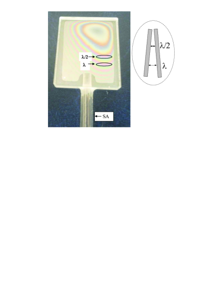
Figure 1: Photograph of the nanometric-thin cell with vertically wedged vapor gap. Regions of $L=\lambda/2=397.5$ nm and $L=\lambda=795$ nm are marked. SA is the sapphire side-arm filled with metallic Rb.

The NTC operated with a special oven with four optical outlets: a pair of in line ports for laser beam transmission and two orthogonal ports to collect the side fluorescence. This geometry allows simultaneous detection of transmission and fluorescence spectra. The oven with the NTC fixed inside was rigidly attached to a translation stage for smooth vertical translation to adjust the needed vapor column thickness without variation of thermal conditions. A thermocouple is attached to the sapphire side arm (SA) at the boundary of metallic Rb to measure the temperature, which determines the vapor pressure. The SA temperature in present experiment was set to $120$ ^∘C, while the windows temperature was kept some $20$ ^∘C higher to prevent condensation. This regime corresponds to Rb atomic density $N=2\times 10^{13}$ cm^-3.

III.2 Experimental arrangement

Sketch of the experimental setup is presented in Fig. 2. The circularly polarized beam of extended cavity diode laser ($\gamma_{L}<1$ MHz) resonant with Rb $D_{1}$ line, after passing through Faraday isolator was focused to a $0.3$ mm diameter spot onto the Rb NTC (2) orthogonally to the cell window. A polarizing beam splitter (PBS) was used to purify initial linear polarization of the laser radiation; a $\lambda/4$ plate (1) was utilized to produce a circular polarization. In the experiments the thicknesses of vapor column $L=\lambda$ and $L=\lambda/2$ have been exploited. The transmission and fluorescence spectra were recorded by photodiodes with amplifiers followed by a four channel digital storage oscilloscope, Tektronix TDS 2014B. To record transmission and fluorescence spectra, the laser radiation was linearly scanned within up to $20$ GHz spectral region covering the studied group of transitions. The linearity of the scanned frequency was monitored by simultaneously recorded transmission spectra of a Fabry-Pérot etalon (not shown). The nonlinearity has been evaluated to be about 1$\%$ throughout the spectral range. About 30$\%$ of the pump power was branched to the reference unit with an auxiliary Rb NTC (6). The fluorescence spectrum of the latter with thickness $L=\lambda/2$ was used as a frequency reference for $B=0$ Sark2004 .
The assembly of oven with NTC inside with $8$ mm longitudinal size was placed between the permanent ring magnets. Magnetic field was directed along the laser radiation propagation direction k ($\textbf{B}\sslash\textbf{k}$). Extremely small thickness of the NTC is advantageous for the application of very strong magnetic fields with the use of permanent magnets having a $2$ mm diameter hole for laser beam passage. Such magnets are unusable for ordinary cm-size cells because of strong inhomogeneity of the magnetic field, while in NTC, the variation of the $B$-field inside the atomic vapor column is several orders less than the applied $B$ value. The permanent magnets are mounted on a $\Pi$-shaped holder with $50\times 50$ mm² cross-section made from soft stainless steel. Additional form-wounded copper coils allow the application of extra $B$ field (up to $\pm 0.1$ T). The $B$-field strength was measured by a calibrated Hall gauge with an absolute imprecision less than $5$ mT throughout the applied $B$-field range.

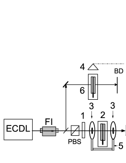
Figure 2: Sketch of the experimental setup. ECDL: diode laser; FI: Faraday isolator; 1: $\lambda/4$ plate; 2: NTC in the oven; PBS: polarizing beam splitter; 3: permanent ring magnets; 4: photodetectors; 5: stainless steel $\Pi$-shape holder; 6: auxiliary Rb NTC with thickness $L=\lambda/2$; BD-beam dumper.

III.3 Realization of the sub-Doppler resolution: “$\lambda$-method” and “$\lambda/2$-method”

Two different methods based on the NTC were implemented to study the behavior of frequency-resolved individual atomic Zeeman transitions exposed to external magnetic field.
1)“$\lambda$-method”. As it was shown in Sark2004 ; Duc , the NTC with thickness of Rb atomic vapor column $L=\lambda$, with $\lambda=795$ nm being the wavelength of the laser radiation resonant with the Rb $D_{1}$ line, is an efficient tool to attain sub-Doppler spectral resolution. Spectrally narrow (10-15 MHz) velocity selective optical pumping (VSOP) resonances located exactly at the positions of atomic transitions appear in the transmission spectrum of NTC at the laser intensities $10$ mW/cm². The VSOP parameters are shown to be immune against 10$\%$ thickness deviation from $L=\lambda$, which makes “$\lambda$-method” feasible. When NTC is placed in a weak magnetic field, the VSOPs are split into several components depending on ($F,m_{F}$), while in the case of strong magnetic fields the VSOPs numbers are determined by the ($J,m_{J};I,m_{I}$) quantum numbers. The amplitudes and frequency positions of VSOPs depend on the $B$-field, which makes it convenient to study separately each individual atomic transition Sarg2008 .
2)“$\lambda$/2-method”. This technique exploits strong narrowing in absorption spectrum at $L=\lambda/2$ as compared with the case of an ordinary cm-size cell [18]. Particularly, the absorption linewidth for Rb $D_{1}$ line reduces to $\sim$ 120 MHz FWHM (Full Width Half Maximum), as opposed to $\sim$ 500 MHz in an ordinary cell. The absorption profile in the case of $L=\lambda/2$ is described by a convolution of Lorentzian and Gaussian profiles (Voigt profile). The sharp (nearly Gaussian) absorption near the top makes it convenient to separate closely spaced individual atomic transitions in an external magnetic field. Also in this case the deviation of thickness by 10$\%$ from $L=\lambda/2$ weakly effects the absorption linewidth. We have used advantages of “$\lambda$-method” and “$\lambda/2$-method” throughout our studies presented below.

IV Consistency of experiment with theoretical considerations

IV.1 Studies for ⁸⁵Rb and ⁸⁷Rb by “$\lambda$-method”: $B=0.5-0.7$ T

The estimates for a $B$-field required to decouple the total electronic angular momentum and the nuclear spin momentum defined by $B\gg B_{0}=A_{hfs}/\mu_{B}$ give $B_{0}=0.07$ T for ⁸⁵Rb and $B_{0}=0.2$ T for ⁸⁷Rb. The recorded transmission spectrum of Rb NTC with thickness $L=\lambda$ for $\sigma^{+}$ laser excitation and $B=0.52$ T is shown in Fig. 3.

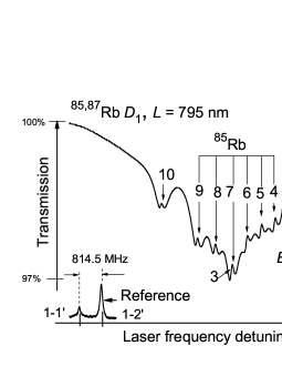
Figure 3: Transmission spectrum of Rb NTC with $L=\lambda$ for $B=0.52$ T and $\sigma^{+}$ laser excitation. The VSOP resonances marked $4-9$ belong to ⁸⁵Rb; resonances marked $1,2,3,10$ belong to ⁸⁷Rb. The lower curve is fluorescence spectrum of the reference NTC with $L=\lambda/2$, showing the positions of ⁸⁷Rb $F_{g}=1\rightarrow F_{e}=1,2$ transitions for $B=0$, labeled as $1-1^{\prime}$ and $1-2^{\prime}$.

The VSOP resonances labeled $1-10$ demonstrate increased transmission at the positions of the individual Zeeman transitions: six transitions, $4-9$, belong to ⁸⁵Rb, and four transitions, $1,2,3,10$ belong to ⁸⁷Rb. VSOPs labeled $3$ and $7$ are overlapped. The larger amplitudes for ⁸⁵Rb components are caused by isotopic abundance in natural Rb (72$\%$ ⁸⁵Rb, 28$\%$ ⁸⁷Rb). The lower curve shows the fluorescence spectrum of the reference NTC with $L=\lambda/2$, showing the positions of ⁸⁷Rb, $F_{g}=1\rightarrow F_{e}=1,2$ transitions. Frequency shifts of all the VSOP peaks are measured from $F_{g}=1\rightarrow F_{e}=2$ transition.

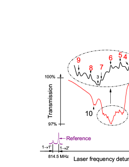
Figure 4: Transmission spectrum of Rb NTC with $L=\lambda$ for $B=0.677$ T and $\sigma^{+}$ laser excitation. The labeling of VSOP resonances is the same as in Fig. 3. All the VSOP resonances are well resolved. The lower curve is the fluorescence spectrum of the reference NTC with $L=\lambda/2$, showing the positions of ⁸⁷Rb $F_{g}=1\rightarrow F_{e}=1,2$ transitions for $B=0$.

The further increase of a $B$-field results in complete resolving of all the transition components (including 3 and 7). The transmission spectrum recorded for $B=0.677$ T, otherwise in the same conditions as in Fig. 3 is presented in Fig. 4.
As it is mentioned above, in the case of HPB regime the eigenstates of the Hamiltonian are described in the uncoupled basis of $J$ and $I$ projections ($m_{J};m_{I}$). Fig. 55 presents a diagram of six Zeeman transitions of ⁸⁵Rb for the HPB regime in the case of $\sigma^{+}$ polarized laser excitation (selection rules: $\Delta m_{J}=+1;\Delta m_{I}=0$), with the same labeling as in Figs. 3,4.

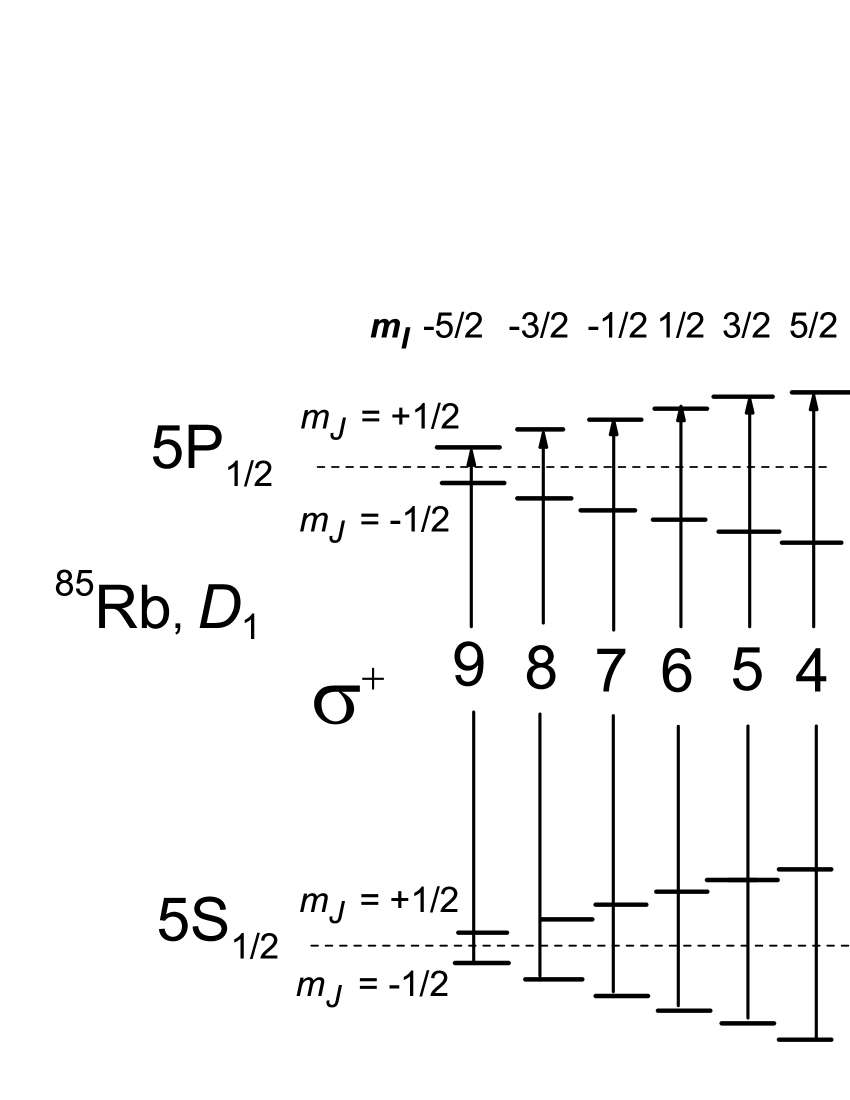
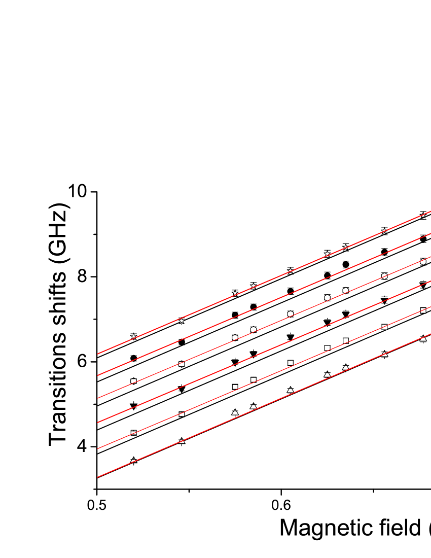
Figure 5: (Color online) a) Diagram of ⁸⁵Rb $D_{1}$ line transitions in the HPB regime for $\sigma^{+}$ laser excitation. b) Magnetic field dependence of the frequency shifts for the transition components $4-9$. Red solid lines $4-9$: calculation by the coupled basis theory; black solid lines $(4)-(9)$: calculation by the HPB theory; symbols: experimental results (measurement inaccuracy is $\pm 1\%$). Note, that the curves 9 and (9) are completely overlapped.

Magnetic field dependence of frequency shift for ⁸⁵Rb components $4-9$ is shown in Fig. 55. Red lines marked $4-9$ are calculated by the coupled basis theory, and black lines $(4)-(9)$ are calculated by the HPB theory, see Eq. 24. Symbols represent the experimental results. As it is seen, for $B>0.6$ T also the theoretical curves for HPB regime well describe the experiment with inaccuracy of $\pm 1\%$.

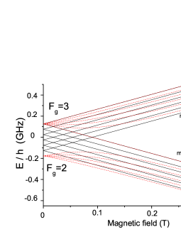
Figure 6: (Color online) Theoretical magnetic field dependence of $F_{g}=2,3$ ground hyperfine levels of ⁸⁵Rb. Red lines: calculations by the coupled basis theory; black lines: calculations as given by Eq.(12) (HPB regime). Ground levels for the transitions $4-9$ are indicated as $(4)_{g}-(9)_{g}$.

Theoretical graphs for splitting of ground state hyperfine levels $F_{g}=2,3$ of ⁸⁵Rb versus magnetic field starting from $B=0$ calculated by coupled and uncoupled basis theories are shown in Fig. 6. Ground sublevels for transitions $4-9$ are indicated as $(4)_{g}-(9)_{g}$. A drastic difference between the two models observed at low magnetic field due to the complete neglecting of the $J-I$ coupling in Eq.(11) gradually reduces with the increase of the $B$-field. Five sublevels of $F_{g}=2$ and seven sublevels of $F_{g}=3$ in coupled basis model (red lines) tend to converge to sublevels of two six-component groups for uncoupled basis model (black lines) with the increase of magnetic field. For $B\geq 0.6$ T, both models become consistent with the experimental results to an accuracy of $\pm 1\%$ (Fig. 55). It is important to note, that for the upper states of transitions $4-9$, the convergence of the two models occurs at much lower magnetic field ($B>0.2$ T), because the hyperfine coupling coefficient $A_{hfs}$ for 5P_1/2 of ⁸⁵Rb is $h\times 120$ MHz, $8$ times smaller than $A_{hfs}$ for 5S_1/2.
Thus, for $B\geq 0.6$ T simple equation (24) could be used for the determination of the following important parameters of ⁸⁵Rb atoms: 1) Frequency positions of atomic transition components and frequency separation $\Delta_{nk}$ of $n$-th and $k$-th atomic transition components:

$$\Delta_{nk}= \big{\{}A_{hfs}\left(P_{1/2}\right)m_{J}\left[m_{I}(n)-m_{I}(k)\right]+$$

$$A_{hfs}\left(S_{1/2}\right)m_{J}\left[m_{I}(n)-m_{I}(k)\right]\big{\}}$$ (33)

Particularly, the frequency distance between $n=4$ and $k=5$ components is $566$ MHz, which coincides with the experimental results at $B>0.6$ T to $2\%$ accuracy. 2) The slope $S$ in dependence of atomic transition components frequency on magnetic field, which is the same for all the $6$ components $4-9$, and can be calculated by the expression

$$S= \left[g_{J}\left(P_{1/2}\right)m_{J}+g_{J}\left(S_{1/2}\right)m_{J}\right]\mu_{B}/B$$

$$\approx 18.6~{}\textmd{{MHz}}/\textmd{mT}$$ (34)

(as $g_{I}\ll g_{J}$ , we ignore $g_{I}m_{I}$ contribution), which coincides well with the experiment.
In Fig. 77 four transitions of ⁸⁷Rb labeled $1-3,10$ are shown for the case of $\sigma^{+}$ polarized laser excitation for the HPB regime (selection rules: $\Delta m_{J}=+1;\Delta m_{I}=0$). The magnetic field dependence of frequency shift for these components is presented in Fig. 77. The red curves $1-3,10$ are calculated by the coupled basis theory, and the black lines $(1)-(3)$ and $(10)$ are calculated by the HPB theory, Eq.(12). Symbols represent the experimental results.

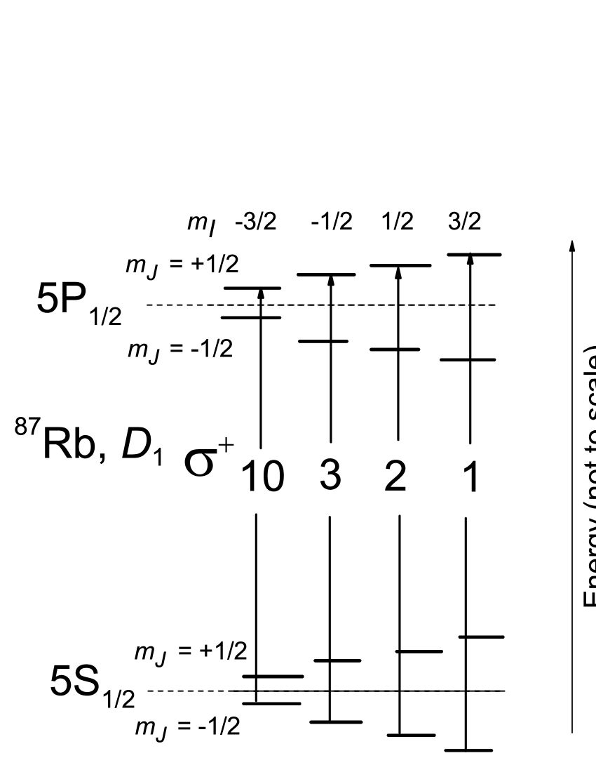
Figure 7: (Color online) a) Diagram of ⁸⁷Rb $D_{1}$ line transitions in the HPB regime for $\sigma^{+}$ laser excitation. b) Magnetic field dependence of the frequency shifts for the transition components $1-3$ and $10$. Red solid lines $1-3,10$: calculation by the coupled basis theory; black solid lines $(1)-(3),(10)$: calculation by the HPB theory; symbols: experimental results (measurement inaccuracy is $\pm 1\%$). Note, that the red curve $10$ and black curve $(10)$ are completely overlapped.

Similar to Fig. 6 and for the same reason, drastic difference between the two models is observed in Fig. 77 for weak magnetic field, with tendency to converge as the $B$-field increases. However, the curves converge at significantly higher magnetic field ($>0.6$ T) required to decouple the nuclear and electronic spins for ⁸⁷Rb having larger hyperfine splitting. It is important to note that also for four transitions of ⁸⁷Rb, the slope $S$ is nearly the same as for ⁸⁵Rb ($S\approx 18.6~{}\textmd{MHz/mT}$). This is explained by the fact that the expression for $S$ contains values of $g_{J}(5S_{1/2})m_{J}$ and $g_{J}(5P_{1/2})m_{J}$ which are the same for ⁸⁵Rb and ⁸⁷Rb, but does not contain $A_{hfs}$ values for $5S_{1/2}$ state that are strongly different.
It is worth noting that the complete HPB regime for Cs $D_{2}$ line having the same ground state $A_{hfs}$ value as for ⁸⁷Rb, has been observed in Hap at $B\sim 2.7$ T. Thus, one may expect that also for ⁸⁷Rb the complete HPB regime appears for $B>10B_{0}$.

IV.2 Studies of hyperfine Paschen-Back regime for ⁸⁵Rb and ⁸⁷Rb by “$\lambda/2$-method”

Advantages of “$\lambda/2$-method” addressed in Section III.3 make it convenient to separate closely spaced individual atomic transitions in an external magnetic field. In order to compare “$\lambda/2$-method” and “$\lambda$-method” (based on VSOP resonance), we have combined in Fig. 8 the spectra obtained by these methods at $B=0.605~{}\textmd{T}$, keeping the previous labeling of individual transitions of ⁸⁵Rb and ⁸⁷Rb. Let us discuss the distinctions of “$\lambda/2$-method” versus “$\lambda$-method”. First, it requires $4$ orders

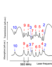
Figure 8: (Color online) Comparison of spectra obtained by “$\lambda$-method” (upper graph) and “$\lambda/2$-method” (lower graph) for $B=0.605$ T.

less laser radiation intensity. In the case of low absorption (a few percent), the absorption $A$ is proportional to $\sigma NL$, where $\sigma$ is the absorption cross-section and is proportional to $d^{2}$ ($d$ being the dipole moment matrix element), $N$ is the atomic density, and $L$ is the thickness. Thus, directly comparing $A_{i}$ (peak amplitudes of the absorption of the $i$-th transition), it is straightforward to estimate the relative probabilities (line intensities). Meanwhile for VSOP-based method the linearity of the response has to be verified. Moreover, spatial resolution is twice better for $L=\lambda/2$ as compared with $L=\lambda$, which can be important when strongly inhomogeneous magnetic field is applied. On the other hand, method based on VSOP provides 5-fold better spectral resolution. Thus, the two methods can be considered as complementary depending on particular requirements. Note that it is easy to switch from $\lambda/2$ to $\lambda$ in experiment just by vertical translation of the NTC.

IV.3 Consistency of coupled basis model with experiment: ⁸⁵Rb

In the frame of coupled basis for $\sigma^{+}$ laser excitation, there are twenty atomic transitions for ⁸⁵Rb according to the selection rules. It should be noted that for $B<20~{}\textmd{mT}$ and $\sigma^{+}$ excitation all the twenty atomic transitions of ⁸⁵Rb have been recorded in Auz . Fig. 9 shows the transition probabilities versus $B$ for nine $F_{g}=2\rightarrow F_{e}=2,3$ transition components under $\sigma^{+}$ excitation (see the labeled diagram in the inset). We can see from Fig. 9 that the probabilities of transitions $4-8$ increase, and probabilities of transitions $9^{\prime}-12^{\prime}$ decrease with $B$, and for $B>0.5~{}\textmd{T}$ only $5$ transitions $(4-8)$ remain in the spectrum.

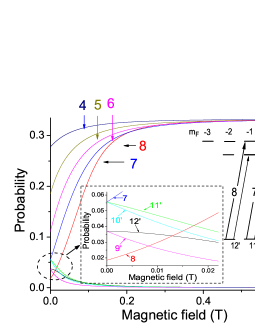
Figure 9: (Color online) The probabilities of nine Zeeman components of $F_{g}=2\rightarrow F_{e}=2,3$ transitions of ⁸⁵Rb $D_{1}$ line labeled in the inset versus $B$ for the case of $\sigma^{+}$ excitation.

Similarly, the probabilities of eleven components of $F_{g}=3\rightarrow F_{e}=2,3$ transitions versus $B$ for the case of $\sigma^{+}$ excitation are presented in Fig. 10. Here only the probability of the transition labeled 9 increases with $B$, remaining the only component in the spectrum for $B>0.5$ T.

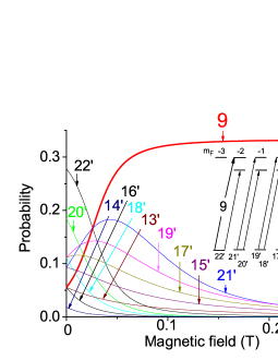
Figure 10: (Color online) The probabilities of nine Zeeman components of $F_{g}=3\rightarrow F_{e}=2,3$ transitions of ⁸⁵Rb $D_{1}$ line labeled in the inset versus $B$ for the case of $\sigma^{+}$ excitation.

Thus, also in the frame of the coupled basis six transitions remain in ⁸⁵Rb $D_{1}$ line spectrum at $B>0.5~{}\textmd{T}$ for $\sigma^{+}$ excitation.
Although the experimental results obtained for strong magnetic field are found to be in consistency with an uncoupled basis model (HPB regime) and can be described by simple theoretical expressions as is shown in Section II, however there are some cases when the coupled basis is to be used. Particularly, it was revealed in Sarg2008 that $F_{g}=1\rightarrow F_{e}=3$ transition “forbidden” at $B=0$ due to the selection rule $\Delta F=0,\pm 1$ appears in the transmission spectrum of ⁸⁷Rb $D_{2}$ line at strong magnetic field. Even for $B>0.6~{}\textmd{T}$, the probability of this transition calculated in the coupled basis is not negligible and can be easily detected.

IV.4 Consistency of coupled basis model with experiment: ⁸⁷Rb

Four atomic transitions of ⁸⁷Rb in HPB regime were presented in Fig. 77. In the frame of coupled basis $(F,m_{F})$ for $\sigma^{+}$ laser excitation there are twelve atomic transitions according to the selection rules, which are presented in Fig. 11. The transitions labeled $1-3$ and $10$ (shown also in Fig. 77) are depicted by solid lines, and other transitions absent for HPB case are presented by dashed lines. Note that for weak magnetic field ($B<20~{}\textmd{mT}$) in the case of $\sigma^{+}$ excitation all twelve atomic transitions of ⁸⁷Rb have been detected in Khv . In order to find out which atomic transitions will remain in a strong magnetic field regime, it is needed to calculate the magnetic field-dependent probabilities for all the twelve atomic transitions. Fig. 12 shows the dependence of the probabilities of atomic transitions $1-5$ on magnetic field for $\sigma^{+}$ laser excitation. It is clearly seen that only transitions $1-3$ remain in the spectrum for $B>0.2$ T.

Figure 11: Diagram of ⁸⁷Rb $D_{1}$ line transitions in the frame of coupled basis for $\sigma^{+}$ laser excitation; the selection rules: $\Delta F=0,1;\Delta m_{F}=+1$.

Figure 12: Calculated probabilities of Zeeman transitions $1-3$, $7^{\prime}$ and $8^{\prime}$ for $\sigma^{+}$ laser excitation versus magnetic field.

The same dependence for transitions labeled $1^{\prime}-6^{\prime}$ and $10$ is shown in Fig. 13. Here only transition 10 remains at $B>0.5~{}\textmd{T}$.

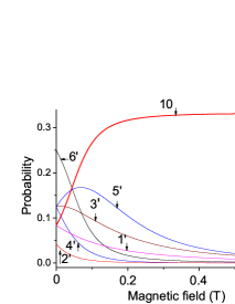
Figure 13: (Color online) Calculated probabilities of Zeeman transitions $1^{\prime}-6^{\prime}$ and $10$ for $\sigma^{+}$ laser excitation versus magnetic field.

Thus, both models give the same result: only transitions $1-3$ and $10$ remain at a strong magnetic field. However, the HPB model is advantageous, being simple and easy for calculations.

V Conclusion

It is demonstrated that simple and efficient “$\lambda$-method” and “$\lambda/2$-method” based on nanometric-thickness cells filled with alkali metal atoms allow to study behavior of atomic Zeeman transitions of ⁸⁵Rb, ⁸⁷Rb $D_{1}$ lines in a wide range of magnetic field from $1$ mT to $1$ T. Particularly, for the case of $\sigma^{+}$ polarized laser radiation and $B>0.5~{}\textmd{T}$, only 6 transitions remain in the transmission spectrum of ⁸⁵Rb $D_{1}$ line, and only $4$ transitions remain in ⁸⁷Rb spectrum. For $B>0.6$ T the expression, which is valid in the frame of uncoupled basis (hyperfine Paschen-Back regime), describes very well the experimental results for ⁸⁵Rb atomic transitions. The latter is important for the determination of such parameters as: the atomic transitions frequency position and frequency separation of the components; the slope $S$ in dependence of atomic transition components frequency on magnetic field can be easily calculated with an inaccuracy of $2\%$. For ⁸⁷Rb having larger hyperfine splitting, the experimental results are very well described in the frame of coupled basis, meanwhile the uncoupled basis model yields inaccuracy of $\sim$ 10$\%$ for the range of $0.5-0.7~{}\textmd{T}$. Consistency of the two models for ⁸⁷Rb are expected to reach at $B\geq 1$ T.
It is worth noting that calculations of magnetic field dependence of Zeeman transition probabilities and frequency positions for the case of $\sigma^{+}$ polarized laser radiation performed in the frame of the coupled basis model are fully consistent with experimental results for all the atomic transitions of ⁸⁵Rb $D_{1}$ line (twenty transitions) and ⁸⁷Rb $D_{1}$ line (twelve transitions) in a broad range of magnetic field ($1~{}\textmd{mT}-1~{}\textmd{T}$). Such calculations will be of interest also for Cs, K, Na, Li.
The results of this study can be used to develop hardware and software solutions for magnetometers with nanometric (400 nm) local spatial resolution and widely tunable frequency reference system based on a NTC and strong permanent magnets.

- (1) J. Keaveney, A. Sargsyan, U. Krohn, D. Sarkisyan, I.G. Hughes, C.S. Adams, Phys. Rev. Lett. 108, 173601 (2012).
- (2) J. Keaveney, I.G. Hughes, A. Sargsyan, D. Sarkisyan, C.S. Adams, Phys. Rev. Lett. 109, 233001 (2012).
- (3) M. Fichet, G. Dutier, A. Yarovitsky, P. Todorov, I. Hamdi, I. Maurin, S. Saltiel, D. Sarkisyan, M.-P. Gorza, D. Bloch, M. Ducloy, Europhys. Lett. 77, 54001 (2007).
- (4) P. Tremblay, A. Michaud, M. Levesque, S. Thériault, M. Breton, J. Beaubien, N. Cyr, Phys. Rev. A 42, 2766 (1990).
- (5) E. B. Aleksandrov, M. P. Chaika, G. I. Khvostenko, Interference of Atomic States (Springer-Verlag, Berlin, ISBN 354053752X, 1993).
- (6) D. Sarkisyan, A. Papoyan, T. Varzhapetyan, K. Blush, M. Auzinsh, J. Opt. Soc. Am. B 22, 88 (2005).
- (7) B. A. Olsen, B. Patton, Y.-Y. Jau, and W. Happer, Phys. Rev. A 84, 063410 (2011).
- (8) M. Auzinsh, D. Budker, S.M. Rochester, Optically Polarized Atoms: Understanding Light-Atom Interactions (Oxford University Press, ISBN 978-0-19-956512-2, 2010).
- (9) L. Weller, K. S. Kleinbach, M. A. Zentile, S. Knappe, Ch.S Adams, I.G. Hughes, J. Phys. B: At. Mol. Opt. Phys. 45, 215005 (2012).
- (10) A. Sargsyan, G. Hakhumyan, A. Papoyan, D. Sarkisyan, A. Atvars, M. Auzinsh, Appl. Phys. Lett. 93, 021119 (2008).
- (11) A. Sargsyan, G. Hakhumyan, C. Leroy, Y. Pashayan-Leroy, A. Papoyan, D. Sarkisyan, Opt. Lett. 37, 1379 (2012).
- (12) D.A. Steck, Rubidium 85 D line data, http://steck.us/alkalidata/rubidium85numbers.pdf; Rubidium 87 D line data, http://steck.us/alkalidata/rubidium87numbers.pdf.
- (13) D. A. Varshalovich, A. N. Moskalev, and V. K. Khersonskii, Quantum theory of angular momentum: irreducible tensors, spherical harmonics, vector coupling coefficients, 3mj symbols (Singapore, Teaneck, USA: World Scientific Pub. 1988) p. 514.
- (14) D. Sarkisyan, D. Bloch, A. Papoyan, M. Ducloy, Opt. Commun. 200, 201 (2001).
- (15) A. Sargsyan, Y. Pashayan-Leroy, C. Leroy, R. Mirzoyan, A. Papoyan, D. Sarkisyan, Appl. Phys. B.: Las. Opt. 105, 767 (2011).
- (16) D. Sarkisyan, T. Varzhapetyan, A. Sarkisyan, Yu. Malakyan, A. Papoyan, A. Lezama, D. Bloch, M. Ducloy, Phys. Rev. A 69, 065802 (2004).
- (17) C. Andreeva, S. Cartaleva, L. Petrov, S.M. Saltiel, D. Sarkisyan, T. Varzhapetyan, D. Bloch, M. Ducloy, Phys. Rev. A 76, 013837 (2007).