Identifying Graphical Models

Abstract

The ability to identify reliably a positive or negative partial correlation between the expression levels of two genes is influenced by the number $p$ of genes, the number $n$ of analyzed samples, and the statistical properties of the measurements. Classical statistical theory teaches that the product of the root sample size multiplied by the size of the partial correlation is the crucial quantity. But this has to be combined with some adjustment for multiplicity depending on $p$, which makes the classical analysis somewhat arbitrary. We investigate this problem through the lens of the Kullback-Leibler divergence, which is a measure of the average information for detecting an effect. We conclude that commonly sized studies in genetical epidemiology are not able to reliably detect moderately strong links.
Keywords: graphical model, partial correlation, Kullback-Leibler divergence

1 Introduction

Probabilistic graphical models are graphs in which nodes represent random variables $X_{u}$ and the edges represent conditional dependence. Any two nodes or variables that are not connected are independent, conditional on the values of all the other random variables. Such models provide a compact representation of a joint probability distribution. In a typical genetical epidemiology application, the variables $X_{u}$ are gene expressions and their measurements are available from tissue samples of $n$ patients. The graphical model is used to describe the association between genes. We write $X_{1}\perp\!\!\!\perp X_{2}|X_{3}\ldots X_{p}$ to indicate that $X_{1}$ and $X_{2}$ are conditionally independent, given $X_{3}\ldots X_{p}$. For the multivariate normal distribution, conditional independence is equivalent to zero entries in the inverse covariance matrix $\Sigma^{-1}$ (also called a concentration or precision matrix). Thus, if $X$ is a $p$-dimensional normal random vector with regular covariance matrix $\Sigma$, then for $1\leq u,v\leq p$ with $u\neq v$

$$X_{u}\perp\!\!\!\perp X_{v}\hskip 5.0pt|\hskip 5.0ptX_{rest}\Longleftrightarrow\sigma^{uv}=0\,,$$

where $\Sigma^{-1}=(\sigma^{uv})_{u,v=1}^{p}$.

Estimating the structure of the concentration matrix from data can be solved with a variety of statistical procedures. A possible approach for low-dimensional data, for example, consists in testing the inclusion of every edge separately, edge by edge. Thus, we have to test $H_{0}^{uv}:\rho_{uv\cdot\text{rest}}=0$ for all $\binom{p}{2}$ choices of $u$ and $v$, where rest refers to the variables with indices in $\{1,2,\ldots,p\}\setminus\{u,v\}$. To study the feasibility of identifying the correct model, we could then investigate how the power of this multiple testing problem depends on $n$ and $p$.

A better way to investigate the feasibility of edge-detection is based on the Kullback-Leibler divergence. The Kullback-Leibler divergence (KLD) measures in a statistically meaningful way the difference between two probability distributions $F_{1}$ and $F_{2}$ with densities $f_{1}$ and $f_{2}$ (see Kullback, 1997). It is defined as

$$D(f_{1}|f_{0})=\mathbb{E}_{X\sim F_{1}}\left[\log\left(\frac{f_{1}(X)}{f_{0}(X)}\right)\right]\,.$$ (1)

The divergence is thus simply the expected value of the log-likelihood-ratio for a single observation $X$ from the alternative model $F_{1}$ when testing the null model $F_{0}$. It is easy to show that this divergence is positive unless $F_{0}=F_{1}$, in which case it is zero. Furthermore, the bigger the KLD, the easier it is to distinguish $F_{1}$ from $F_{0}$ by likelihood tests and the more powerful the test will be (for details, see Morgenthaler and Staudte, 2012). If we dispose of $n$ independent observations, the KLD is multiplied by $n$. If we test the absence of partial correlations vs. the presence of partial correlations and assume multivariate Gaussianity, the KLD is a useful tool to determine the average amount of information in the data. Because it is based on likelihoods rather than estimates, the KLD can be computed for any two models, without reference to additional conditions such as $n>p$. This is an advantage of this approach.

In the remainder of the paper, we will examine how information accumulates when trying to fit a graphical model. When testing for edges, we will be interested in the power of the test and the traditional asymptotic analysis is not valid when $p>n$, while in the KLD approach, we can directly compute the relevant amount of information.

2 The Kullback-Leiber divergence

Suppose we have two $p$-variate normal populations with densities

$$f_{i}(x_{1},\ldots,x_{p})=\frac{1}{\displaystyle|2\pi\Sigma_{i}|^{1/2}}\exp(-\tfrac{1}{2}(x-\mu_{i})^{T}\Sigma_{i}^{-1}(x-\mu_{i}))\text{ for }i=0,1\,,$$ (2)

where $x=(x_{1},\ldots,x_{p})$ and $\mu_{i},\Sigma_{i}$ denote the multivariate means and covariance matrices. It follows that

$$\log\left(\displaystyle\frac{f_{1}(x)}{f_{0}(x)}\right)=\tfrac{1}{2}\log\left(\frac{|\Sigma_{1}|}{|\Sigma_{0}|}\right)-\tfrac{1}{2}\text{tr}\Sigma_{0}^{-1}(x-\mu_{0})(x-\mu_{0})^{T}\\ +\tfrac{1}{2}\text{tr}\Sigma_{1}^{-1}(x-\mu_{1})(x-\mu_{1})^{T}\,.$$

Taking the expectation of the above, we can evaluate (1) as

$$D(f_{1}|f_{0})=\tfrac{1}{2}\log\left(\frac{|\Sigma_{1}|}{|\Sigma_{0}|}\right)+\tfrac{1}{2}\text{tr}\Sigma_{0}(\Sigma_{1}^{-1}-\Sigma_{0}^{-1})+\tfrac{1}{2}\text{tr}\Sigma_{1}^{-1}(\mu_{0}-\mu_{1})(\mu_{0}-\mu_{1})^{T}\,.$$ (3)

We will make use of this formula for our purpose in which normal populations with equal means but unequal covariance matrices are compared. The null model will have a covariance matrix equal to the identity matrix, while the alternative model will have a covariance matrix whose inverse is nearly equal to the identity matrix. This describes a situation where the $p$ variables have equal variance and only a very small proportions of all partial correlations are non-zero.

2.1 Divergence for a single non-zero partial correlation with known placement

Let $f_{uv}$ and $f_{0}$ be $p$ dimensional multivariate Gaussian densities with mean $0$ and variances $\Sigma_{uv}$, $I_{p}$ (identity matrix ), respectively. For now, the matrix $\Sigma_{uv}^{-1}$ has diagonal elements equal to 1 and all off-diagonal values are zero, except for a value of $\rho\neq 0$ in positions $(u,v)$ and $(v,u)$, that is, exactly one partial correlation is non-zero. It is easy to show that the partial correlation is equal to $-\rho$ in this case. We will write $\Sigma_{uv}^{-1}=I_{p}+U_{uv}$, where $U_{uv}$ contains the off-diagonal elements of $\Sigma_{uv}$. To compute the divergence (3), we need the determinant of $\Sigma_{uv}^{-1}$ and the trace of $\Sigma_{uv}$, which are

$$|\Sigma_{uv}^{-1}|=1+(-1)^{u+v}\rho(-1)^{v-1+u}\rho=1+\rho^{2}(-1)^{2u+2v-1}=1-\rho^{2}$$

and $\text{trace}(\Sigma_{uv})=p-2+2/(1-\rho^{2})$. Note that the determinant does not depend on the position $(u,v)$, nor does it depend on the dimension $p$, while for the trace the diagonal elements of $\Sigma_{uv}$ are needed. They are are equal to 1, except in positions $(u,u)$ and $(v,v)$, where they are $1/(1-\rho^{2})$. From the previous expression (3) we then find

$$D(f_{uv}|f_{0})=\frac{\log(1-\rho^{2})}{2}+\frac{\rho^{2}}{1-\rho^{2}}\,.$$ (4)

A sample of $n$ observations drawn from the alternative model $f_{uv}$ has an information content in favor of rejecting the null model $f_{0}$ of $nD(f_{uv}|f_{0})$, which tends to infinity as $n$ grows larger. This is true for any value $\rho\neq 0$. For a large enough sample, even a slight partial correlation between the u-th and v-th variable will for sure be detected.

2.2 Divergence when the placement is unknown

In our formulation of the density $f_{uv}$, we of course make use of the knowledge of the placement of the positive partial correlation. Because of this, Eq. (4) is only useful in understanding the null hypothesis $H_{0}^{uv}$, which is only one of the possibilities one has to examine in practice. How does the divergence change if we do not know the pair of correlated variables? To answer this question, we consider a different alternative model, namely the multivariate mixture density

$$f_{1}(x_{1},\ldots,x_{p})=\sum_{u=1}^{p-1}\sum_{v=u+1}^{p}\frac{1}{\binom{p}{2}}f_{uv}(x_{1},\ldots,x_{p})\,.$$ (5)

In this case, the following result holds.

Theorem 1

The amount of information about $\rho$ in a sample of size $n$ drawn from the mixture distribution (5), information in favor of distinguishing this mixture model from the null model of independent standard normals, is for $|\rho|<1/\sqrt{2}$ and large dimension $p$ equal to

$$nD(f_{1}|f_{0})=\frac{4n}{p}\left(\frac{1-\rho^{2}}{\sqrt{1-2\rho^{2}}}-1\right)+o(p^{-1})\,.$$ (6)

Proof 1

Since

$$f_{uv}(x_{1},\ldots,x_{p})=\frac{\sqrt{1-\rho^{2}}}{(2\pi)^{p/2}}\exp\left(-\frac{1}{2}(x_{1}^{2}+\ldots+x_{p}^{2}+2\rho x_{u}x_{v})\right)\,,$$

the likelihood ratio is equal to

$$\frac{f_{1}(x)}{f_{0}(x)}=\frac{\displaystyle\frac{\sqrt{1-\rho^{2}}}{{p\choose 2}}\sum_{u=1}^{p-1}\sum_{v=u+1}^{p}\exp\left(-\tfrac{1}{2}(x_{1}^{2}+\ldots+x_{p}^{2}+2\rho x_{u}x_{v})\right)}{\displaystyle\exp(-\tfrac{1}{2}(x_{1}^{2}+\cdots+x_{p}^{2}))}\\ ={\displaystyle\frac{\sqrt{1-\rho^{2}}}{{p\choose 2}}\sum_{u=1}^{p-1}\sum_{v=u+1}^{p}\exp(-\rho{x_{u}}{x_{v}})}\,,$$

where as before $x=(x_{1},\ldots,x_{p})$. It follows that

$$D(f_{1}|f_{0})=\int_{\mathbb{R}^{p}}\log\left(\frac{f_{1}(x)}{f_{0}(x)}\right)f_{1}(x)\,dx\\ =\int_{\mathbb{R}^{p}}\log\left({\displaystyle\frac{\sqrt{1-\rho^{2}}}{{p\choose 2}}\sum_{u=1}^{p-1}\sum_{v=u+1}^{p}\exp(-\rho{x_{u}}{x_{v}})}\right)f_{1}(x)\,dx\\ =\int_{\mathbb{R}^{p}}\log\left({\displaystyle\frac{\sqrt{1-\rho^{2}}}{{p\choose 2}}\sum_{u=1}^{p-1}\sum_{v=u+1}^{p}\exp(-\rho{x_{u}}{x_{v}})}\right)f_{12}(x)\,dx\,,$$ (7)

where the last equality follows from the fact that the ratio of the densities is invariant with respect to permutations of the components of $x$.

The expectation (7) can be approximated for large dimensions $p$ via the law of large numbers. Let $(X_{1},\ldots,X_{p})$ be a random vector with density $f_{12}$. It follows that if $(Z_{1},\ldots,Z_{p})$ are independent unit Gaussian random variables, we have the representation $(X_{1}=AZ_{1}+BZ_{2},X_{2}=AZ_{2}+BZ_{1},X_{3}=Z_{3},\ldots,X_{p}=Z_{p})$, where $A=(1+[(1+\rho)/(1-\rho)]^{1/2})/(2(1+\rho)^{1/2})$ and $B=(1-[(1+\rho)/(1-\rho)]^{1/2})/(2(1+\rho)^{1/2})$. The integrand in (7) can thus be written as

$$\log\left(\frac{\sqrt{1-\rho^{2}}}{{p\choose 2}}\left(e^{-\rho{X_{1}}{X_{2}}}+\sum_{v=3}^{p}\left(e^{-\rho X_{1}Z_{v}}+e^{-\rho X_{2}Z_{v}}\right)+\sum_{u=3}^{p-1}\sum_{v=i+1}^{p}e^{-\rho Z_{u}Z_{v}}\right)\right)\\ =\log\Bigg{(}\sqrt{1-\rho^{2}}\Bigg{(}O_{P}(p^{-2})+\frac{2}{p^{2}-p}\left(\sum_{v=3}^{p}\left(e^{-\rho X_{1}Z_{v}}+e^{-\rho X_{2}Z_{v}}\right)\right)\\ +\frac{2}{p^{2}-p}\left(\sum_{u=3}^{p-1}\sum_{v=i+1}^{p}e^{-\rho Z_{u}Z_{v}}\right)\Bigg{)}\Bigg{)}\,.$$ (8)

For large $p$, the two last terms can be approximated by their asymptotic limits. The product of two independent normal variables, which appears in these expressions, has surprising properties (see Aroian, 1947). Elementary calculations show that if $Z_{1},Z_{2}$ are independent with a unit Gaussian distribution, then $\mathbb{E}[\exp(-\rho Z_{1}Z_{2})]=(1-\rho^{2})^{-1/2}$. With $Y=\exp(-\rho Z_{1}Z_{2})$ we thus find for $\gamma>0$ that $\mathbb{E}[|Y|^{\gamma}]=\mathbb{E}[\exp(-\gamma\rho Z_{1}Z_{2})]=(1-\rho^{2}\gamma^{2})^{-1/2}$, which is finite if $|\rho|\gamma<1$. For $0<|\rho|<0.5$, this allows a maximal value $\gamma\geq 2$ (finite variance), while for $0.5\leq|\rho|<1$, we always have a maximal value $1<\gamma<2$ (infinite variance).

With regard to the last term in (8), this shows that for all $\rho\neq 0$ we have convergence in probability of the mean

$$\hskip 28.45274pt\binom{p}{2}^{-1}\left(\sum_{u=3}^{p-1}\sum_{v=i+1}^{p}e^{-\rho Z_{u}Z_{v}}\right)=\\ \left(1-\frac{4}{p}+O(p^{-2})\right)\binom{p-2}{2}^{-1}\left(\sum_{u=3}^{p-1}\sum_{v=i+1}^{p}e^{-\rho Z_{u}Z_{v}}\right)\overset{\text{in P}}{\longrightarrow}\frac{1}{\sqrt{1-\rho^{2}}}\text{ as }p\to\infty\,,$$

but the rate of convergence in the law of large numbers depends on the value of $\rho$.

The other term in (8) involves either $X_{1}$ or $X_{2}$, which both have variance $(1-\rho^{2})^{-1}$ and have the same marginal distribution as $Z_{1}(1-\rho^{2})^{-1/2}$. It follows that the typical summand is $Y=\exp(-\rho(1-\rho^{2})^{-1/2}Z_{1}Z_{2})$, which for $\gamma>0$ satisfies $\mathbb{E}[|Y|^{\gamma}]=\mathbb{E}[\exp(-\gamma\rho(1-\rho^{2})^{-1/2}Z_{1}Z_{2})]=(1-\rho^{2}\gamma^{2}/(1-\rho^{2}))^{-1/2}$. This is only finite, if $\gamma^{2}<(1-\rho^{2})/\rho^{2}$. For $|\rho|<0.5$, $\gamma$ takes values up to at least $\sqrt{3}$ and for $|\rho|<1/\sqrt{5}$, the variance is finite, that is, $\gamma$ is at least 2. For $|\rho|>1/\sqrt{2}$, $\gamma$ is less than 1 and the expected value becomes infinite. In the range of $\rho$ values we are considering, the expectation is equal to $(1-\rho^{2}/(1-\rho^{2}))^{-1/2}=[(1-\rho^{2})/(1-2\rho^{2})]^{1/2}$ and thus

$$\binom{p}{2}^{-1}\left(\sum_{v=3}^{p}e^{-\rho X_{1}Z_{v}}\right)=\left(\frac{2}{p}+O(p^{-2})\right)\frac{1}{p-2}\left(\sum_{v=3}^{p}e^{-\rho X_{1}Z_{v}}\right)$$

and

$$\frac{1}{p-2}\left(\sum_{u=3}^{p}e^{-\rho X_{1}Z_{v}}\right)\overset{\text{in P}}{\longrightarrow}\sqrt{\frac{1-\rho^{2}}{1-2\rho^{2}}}\text{ as }p\to\infty\,.$$

Substitution of the limit as an approximate value for large $p$ leads to the following expansion of the value inside the logarithm of (8)

$$\sqrt{1-\rho^{2}}\left(\frac{4}{p}\frac{\sqrt{1-\rho^{2}}}{\sqrt{1-2\rho^{2}}}+\left(1-\frac{4}{p}\right)\frac{1}{\sqrt{1-\rho^{2}}}\right)\\ =1-\frac{4}{p}+\frac{4}{p}\frac{1-\rho^{2}}{\sqrt{1-2\rho^{2}}}\,.$$

Expanding the logarithm to the required order leads to the approximate KLD value claimed in the theorem.

3 Discussion and extensions

3.1 Other values of $\rho$ and numerical comparisons

As the value of $|\rho|$ increases towards 1, the approximate computation of the KDL undergoes several transitions. For the main term in (8) the only point of transition occurs at $\rho=0.5$, when the variance becomes infinite. For the minor term they occur at $\rho=1/\sqrt{5}$, when the variance becomes infinite and at $\rho=1/\sqrt{2}$, when the expectation becomes infinite. At this second point, our formula is no longer valid, because the terms of order $p^{-1}$ are not the leading terms. In this case, a more refined analysis of the tail probabilities of the law of $Y$ is required (see, for example, Gut, 2004; Baum and Katz, 1965; Feller, 1945).

Figure 1 includes the numerical results for $\rho=0.9$. The plot makes it clear that in this case the information content decreases less rapidly with increasing dimension $p$. Even in this case, the linearity in the plot of log(KLD) as a function of log(p) remains, but the slope passes from $-1$ to $-0.25$. The analysis based on moments of $Y$ suggests for $|\rho|>1/\sqrt{2}$ an order of $p^{-\tau}$ with $0<\tau<2(1-\rho^{2})$ (see Baum and Katz, 1965, Theorem 1).

Figure 1 compares the values obtained by Monte Carlo sampling with the approximation given in Theorem 1. The agreement is quite good.

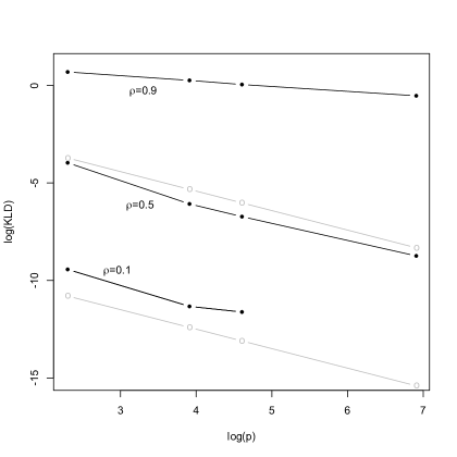
Figure 1: The comparison of the numerical (black) and the approximate (grey) divergence values show a good agreement, even for $p=10$. The approximate divergence decreases as 1/p, which translates into a slope of $-1$ in our plot.

3.2 Classical asymptotics

The analysis using the KLD is related, but different, from the more widely known asymptotic or local power. When using the KLD, there is no correction for multiplicity involved, no constraints of the type $n>p$ are needed and no limits towards infinite study sizes are taken. The KLD thus provides a more solid foundation for judgeing the sample sizes needed in order to reliably detect effects. Here we briefly compare it with the traditional asymptotic approach, where $n\to\infty$ (and implicitly $n>p$). When testing the null hypothesis $H_{0}^{uv}:\rho_{uv\cdot\text{rest}}=0$ against one-sided alternatives $\rho_{uv\cdot\text{rest}}>0$ based on the estimator $s_{uv\cdot\text{rest}}$ and the Bonferroni correction for the number of tests $m=p(p-1)/2$, the power function for large sample sizes is approximately equal to

$$1-\Phi\left(z_{1-\alpha/m}-\sqrt{n}\rho_{uv\cdot\text{rest}}\right)=\Phi\left(\sqrt{n}\rho_{uv\cdot\text{rest}}-z_{1-\alpha/m}\right)\,,$$ (9)

where $z_{1-\alpha/m}$ denotes the $1-\alpha/m$ quantile of the standard normal distribution. Using the asymptotic approximation for this quantile $z_{1-\alpha/m}\sim\sqrt{2\log(m/\alpha)}$, leads to the following one-sided local asymptotic power at the alternative $\rho_{uv\cdot\text{rest}}>0$:

$$\Phi\left(\sqrt{n}\rho_{uv\cdot\text{rest}}-\sqrt{2\log\left[p(p-1)/(2\alpha)\right]}\right)\,,$$ (10)

which depends on $p$ via the logarithm. The above approximation of the quantile $z_{1-\alpha/m}$ is quite crude and gives values that are typically too large so that the power might be underestimated. This local asymptotic approximation is based on the asymptotic normality of the estimator of the partial correlation and on the consideration of alternatives close to the null hypothesis (see for example Chapter 10 of Serfling, 1980). Finding the approximate power involves the calculation of the slope and is based on the expected value of the partial correlation estimate. This can be shown to be (equation (18), section 5.1 in Muirhead, 1982)

$$\frac{2}{f}\,(\Gamma[(f+1)/2]/\Gamma[f/2])^{2}\,\rho_{uv\cdot\text{rest}}~{}_{2}F_{1}\left[\tfrac{1}{2},\tfrac{1}{2};(f+2)/2,\rho^{2}_{uv\cdot\text{rest}}\right],$$

where $f=n+1-p$ and $~{}_{2}F_{1}[\cdot]$ is a hypergeometric function, which is evaluated at $\rho_{uv\cdot\text{rest}}$. It follows that its derivative with respect to $\rho_{uv\cdot\text{rest}}$, evaluated at $\rho_{uv\cdot\text{rest}}=0$, is equal to $2(\Gamma[f/2])^{2}/(f\Gamma[(f+1)/2]^{2})$, which tends to 1 as $f\to\infty$ by Stirling’s approximation. Because the asymptotic variance of the partial correlation estimator assuming that the null hypothesis is true is $1$, the slope of the test or its Pitman efficacy is equal to 1.

A comparison between (6) and (10) can be based on the fact that in order to reach a power of about 0.5 at level $\alpha$, the KLD of an experiment must exceed $z_{1-\alpha}^{2}$ (see Morgenthaler and Staudte, 2012). From this, one can derive a formula for the needed size of a study, $n=pz_{1-\alpha}^{2}/[4((1-\rho^{2})/\sqrt{1-2\rho^{2}}-1)]$. The equivalent value of $n$ from the asymptotic power on the other hand predicts that $n=(z_{1-\alpha/m}/\rho)^{2}$, where $m=p(p-1)/2$ is the number of tests. For values of $\rho<0.5$, the KLD-based formula gives much higher values of the study size $n$. For example, around $n=20,000$ subjects would be required to detect a partial correlation in a single pair of $p=1000$ genes. The asymptotic power wrongly suggests that $n=135$ subjects would be sufficient. Generally speaking, when $\rho<0.5$ the problem of identifying a partial correlation is hopeless, unless the number of candidate genes that are tested can be reduced below $p=100$. Figure 1 also gives an indication of what will happen for a strong effect, $\rho=0.9$. The value of KLD decreases by about a factor of 0.24 for each increase of $p$ by a factor of 10. If we extrapolate to $p=10^{6}$, we have a KLD value of about $8\times 10^{-3}$. We thus would need a study involving at least $n=330$ subjects, which is doable.

3.3 Detecting correlations

The model in which the covariance matrix is equal to our precision matrix, that is, the model with $p$ measurements with equal variance and a single non-null covariance $\rho$ has been analyzed by Arias-Castro et al. (2012). In computations not shown here, we obtain the following result which holds for small values of $\rho$ and large values of $p$

$$nD(f_{1}|f_{0})=\frac{2n}{p^{2}}\left(\frac{1}{\sqrt{1-\rho^{2}}}-1\right)+o(p^{-2})\,.$$

Since the order of the leading term is $p^{-2}$, the detection is this model is nearly impossible unless $n$ is very large.

3.4 Divergence for two partial correlations

If the we consider the alternative multivariate Gaussian model with an inverse covariance matrix in which the diagonal elements are 1 and exactly two pairs of variables have a partial correlation of $\rho$, then the following result holds for $|\rho|<1/\sqrt{2}$

$$nD(f_{1}|f_{0})=\frac{16n}{p}\left(\frac{1-\rho^{2}}{\sqrt{1-2\rho^{2}}}-1\right)+o(p^{-1})\,.$$

Figure 2 shows the qualitative behavior of the three functions we computed. Note that in the case of a perturbation of the correlation matrix by a single non-null element, the information increases very slowly and is of order $O(n/p^{2})$, while a perturbation on the level of the precision matrix leads to $O(n/p)$. If two couples are correlated with an equal correlation rather than a single couple, the information gain is four-fold.

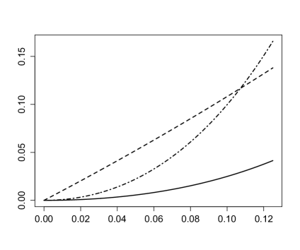
Figure 2: The qualitative behavior of the Kullback-Leibler divergence in the three cases discussed in this paper are shown here. The horizontal axis is equal to the square $\rho^{2}$. The solid curve is the case of a change a single off-diagonal element in the precision matrix, while the dashed curve is a single off-diagonal element in the correlation matrix. In both cases, the diagonal elements of the matrix are all equal to one. The dotted/dashed curve is the case of two non-null and equal elements in the precision matrix.

References

- Arias-Castro et al. (2012) Arias-Castro, E., S. Bubeck, and G. Lugosi (2012). Detection of correlations. The Annals of Statistics 40, 412–435.
- Aroian (1947) Aroian, L. (1947). The probability function of the product of two normally distributed variables. The Annals of Mathematical Statistics 18, 265–271.
- Baum and Katz (1965) Baum, L. E. and M. Katz (1965). Convergence rates in the law of large numbers. Transactions of the American Mathematical Society 120, 108–123.
- Feller (1945) Feller, W. (1945). Note on the law of large numbers and ”fair” games. The Annals of Mathematical Statistics 16, 301–304.
- Gut (2004) Gut, A. (2004). An extension of the kolmogorov–feller weak law of large numbers with an application to the st. petersburg game. Journal of Theoretical Probability 17, 769–779.
- Kullback (1997) Kullback, S. (1997). Information Theory and Statistics. Dover Publications.
- Morgenthaler and Staudte (2012) Morgenthaler, S. and R. G. Staudte (2012). Advantages of variance stabilization. Scandinavian Journal of Statistics 39(4), 714–728.
- Muirhead (1982) Muirhead, R. (1982). Aspects of multivariate statistical theory. John Wiley and Sons, New York.
- Serfling (1980) Serfling, R. J. (1980). Approximation Theorems of Mathematical Statistics. Wiley.