3-D Visual Coverage Based on Gradient Descent Techniques on Matrix Manifold and Its Application to Moving Objects Monitoring

Abstract

This paper investigates coverage control for visual sensor networks based on gradient descent techniques on matrix manifolds. We consider the scenario that networked vision sensors with controllable orientations are distributed over 3-D space to monitor 2-D environment. Then, the decision variable must be constrained on the Lie group $SO(3)$. The contribution of this paper is two folds. The first one is technical, namely we formulate the coverage problem as an optimization problem on $SO(3)$ without introducing local parameterization like Eular angles and directly apply the gradient descent algorithm on the manifold. The second technological contribution is to present not only the coverage control scheme but also the density estimation process including image processing and curve fitting while exemplifying its effectiveness through simulation of moving objects monitoring.

I Introduction

Aspirations for safety and security of human lives against crimes and natural disasters motivate us to establish smart monitoring systems to monitor surrounding environment. In this regard, vision sensors are expected as powerful sensing components since they provide rich information about the outer world. Indeed, visual monitoring systems have been already commoditized and are working in practice. Typically, in the current systems, various decision-making and situation awareness processes are conducted at a monitoring center by human operator(s), and partial distributed computing at each sensor is, if at all, done independently of the other sensors. However, as the image stream increases, it is desired to distribute the entire process to each sensor while achieving total optimization through cooperation among sensors.

Distributed processing over the visual sensor networks is actively studied in recent years motivated by a variety of application scenarios [1]–[10]. Among them, several papers address optimal monitoring of the environment assuming mobility of the vision sensors [4]–[10], where it is required for the network to ensure the best view of a changing environment [4]. The problem is related to coverage control [11]–[13], whose objective is to deploy mobile sensors efficiently in a distributed fashion. A typical approach to coverage control is to employ the gradient descent algorithm for an appropriately designed aggregate objective function. The objective function is usually formulated by integrating the product of a sensing performance function of a point and a density function indicating the relative importance of the point. The approach is also applied to visual coverage in [4]–[6]. The state of the art of coverage control is compactly summarized in [4], and a survey of related works in the computer vision society is found in [15].

In this paper, we consider a visual coverage problem under the situation where vision sensors with controllable orientations are distributed over the 3-D space to monitor 2-D environment. In the case, the control variables i.e. the rotation matrices must be constrained on the Lie group $SO(3)$, which distinguishes the present paper from the works on 2-D coverage [5]–[8]. On the other hand, [4, 9, 10] consider situations similar to this paper. [9, 10] take game theoretic approaches which allow the network to achieve globally optimal coverage with high probability but instead the convergence speed tends to be slower than the standard gradient descent approach. In contrast, [4] employs the gradient approach by introducing a local parameterization of the rotation matrix and regarding the problem as optimization on a vector space.

This paper approaches the problem differently from [4]. We directly formulate the problem as optimization on $SO(3)$ and apply the gradient descent algorithm on matrix manifolds [16]. This approach will be shown to allow one to parametrize the control law for a variety of underactuations imposed by the hardware constraints. This paper also addresses density estimation from acquired data, which is investigated in [14] for 2-D coverage. However, we need to take account of the following characteristics of vision sensors: (i) the sensing process inherently includes projection of 3-D world onto 2-D image, and (ii) explicit physical data is not provided. To reflect (i), we incorporate the projection into the optimization problem on the embedding manifold of $SO(3)$. The issue (ii) is addressed technologically, where we present the entire process including image processing and curve fitting techniques. Finally, we demonstrate the utility of the present coverage control strategy through simulation of moving objects monitoring.

Preliminary: Gradient on Riemannian Manifold

Let us consider a Riemannian manifold ${\mathcal{M}}$ whose tangent space at $x\in{\mathcal{M}}$ is denoted by $T_{x}{\mathcal{M}}$, and the corresponding Riemannian metric, an smooth inner product, defined over $T_{x}{\mathcal{M}}$ is denoted by $\langle\cdot,\cdot\rangle_{x}$. Now, we introduce a smooth scalar field $f(\cdot):{\mathcal{M}}\to{\mathbb{R}}$ defined over the manifold ${\mathcal{M}}$, and the derivative of $f$ at an element $x\in{\mathcal{M}}$ in the direction $\xi\in T_{x}{\mathcal{M}}$, denoted by $Df(x)[\xi]$. We see from Definition 3.5.1 and (3.15) of [16] that the derivative $Df(R)[\Xi]$ is defined by

$$Df(x)[\xi]=\left.\frac{df(\gamma(t))}{dt}\right|_{t=0},$$

where $\gamma:{\mathbb{R}}\to{\mathcal{M}}$ is a smooth curve such that $\gamma(0)=x$. In particular, when ${\mathcal{M}}$ is a linear manifold with $T_{x}{\mathcal{M}}={\mathcal{M}}$, the derivative $Df(R)[\Xi]$ is equal to the classical directional derivative

$$Df(x)[\xi]=\lim_{t\to 0}\frac{f(x+t\xi)-f(x)}{t}.$$ (1)

Now, the gradient of $f$ is defined as follows.

Definition 1

[16] Given a smooth scalar field $f$ defined over a Riemannian manifold ${\mathcal{M}}$, the gradient of $f$ at $x$, denoted by ${\rm grad}_{x}^{{\mathcal{M}}}f$, is defined as the unique element of $T_{x}{\mathcal{M}}$ satisfying

$$\langle{\rm grad}_{x}^{{\mathcal{M}}}f,\xi\rangle_{x}=Df(x)[\xi]\ \ {\forall\xi}\in T_{x}{\mathcal{M}}.$$

Suppose now that ${\mathcal{M}}$ is a Riemannian submanifold of a Riemannian manifold $\mathcal{N}$, namely $T_{x}{\mathcal{M}}$ is a subspace of $T_{x}\mathcal{N}$ and they share a common Riemannian metric. In addition, the orthogonal projection of an element of $T_{x}\mathcal{N}$ onto $T_{x}{\mathcal{M}}$ is denoted by $P_{x}:T_{x}\mathcal{N}\to T_{x}{\mathcal{M}}$. Then, the following remarkable lemma holds true.

Lemma 1

[16] Let $\bar{f}$ be a scalar field defined over $\mathcal{N}$ such that the function $f$ defined on ${\mathcal{M}}$ is a restriction of $\bar{f}$. Then, the gradient of $f$ satisfies the equation

$${\rm grad}_{x}^{{\mathcal{M}}}f=P_{x}{\rm grad}_{x}^{\mathcal{N}}\bar{f}.$$ (2)

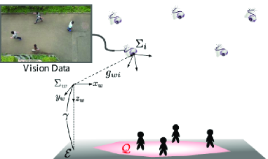
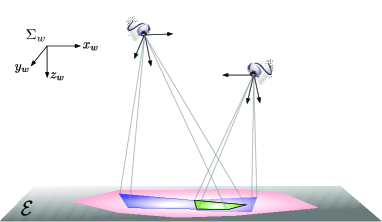
Figure 1: Targeted scenario.

II Targeted Scenario

II-A Vision Sensors and Environment

We consider the situation illustrated in Fig. 1 where $n$ vision sensors ${\mathcal{V}}=\{1,\cdots,n\}$ are located in 3-D Euclidean space. Let the fixed world frame be denoted by $\Sigma_{w}$ and the body fixed frame of sensor $i\in{\mathcal{V}}$ by $\Sigma_{i}$. We also denote the position vector of the origin of $\Sigma_{i}$ relative to $\Sigma_{w}$ by $p_{wi}\in{\mathbb{R}}^{3}$, and the rotation matrix of $\Sigma_{i}$ relative to $\Sigma_{w}$ by $R_{wi}\in SO(3):=\{R\in{\mathbb{R}}^{3\times 3}|\ RR^{T}=R^{T}R=I_{3},\ \det(R)=+1\}$. Then, the pair $g_{wi}=(p_{wi},R_{wi})\in SE(3):={\mathbb{R}}^{3}\times SO(3)$, called pose, represents the configuration of sensor $i$. In this paper, each sensor’s position $p_{wi}$ is assumed to be fixed, and sensors can control only their orientations $R_{wi}$. In addition, we suppose that sensors are localized and calibrated a priori and $g_{wi}$ is available for control.

We use the notation $g_{wi}$ to describe not only the pose but also a coordinate transformation operator similarly to [19]. Take two frames $\Sigma_{a}$ and $\Sigma_{b}$. Let the pose of the frame $\Sigma_{b}$ relative to $\Sigma_{a}$ be denoted by $g_{ab}=(p_{ab},R_{ab})$, and the coordinates of a point relative to $\Sigma_{a}$ by $p_{b}$. Then, the coordinates $p_{a}$ of the point relative to $\Sigma_{a}$ are given as

$$p_{a}=g_{wi}(p_{b}):=R_{ab}p_{b}+p_{ab}.$$

Let us next define the region to be monitored by a group of sensors ${\mathcal{V}}$. In this paper, we assume that the region is a subset of a 2-D plane (Fig. 1), where the 2-D plane is called the environment and the subset to be monitored is called the mission space. Let the set of coordinates of all points in the environment and the mission space relative to $\Sigma_{w}$ are respectively denoted by ${\mathcal{E}}$ and ${\mathcal{Q}}$. Just for simplicity, we suppose that the world frame $\Sigma_{w}$ is attached so that its $x,y$-plane is parallel to the environment (Fig. 1). Then, the set ${\mathcal{E}}$ is formulated as

$${\mathcal{E}}=\{q\in{\mathbb{R}}^{3}|\ {\bf e}_{3}^{T}q=\gamma\}$$

with some constant $\gamma\in{\mathbb{R}}$, where ${\bf e}_{i}\in{\mathbb{R}}^{3},\ i=1,2,3$ is an $i$-th standard basis. Suppose that a metric $\phi:{\mathcal{E}}\to{\mathbb{R}}_{+}$, called a density function, indicating the relative importance of every point $q\in{\mathcal{E}}$ is defined over ${\mathcal{E}}$. In this paper, the function $\phi(q)$ is assumed to be small if point $q$ is important and to satisfy $\phi(q)=\bar{\phi}\ {\forall q}\notin{\mathcal{Q}}$ with a constant $\bar{\phi}$ such that $\bar{\phi}>\sup_{q\in{\mathcal{Q}}}\phi(q)$.

II-B Geometry

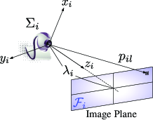
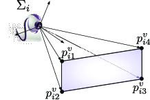
A vision sensor has an image plane containing the sensing array, whose elements, called pixels, provide the numbers reflecting the amount of light incident. We assume that the image plane is a rectangle as illustrated in Fig. 3. The set of position vectors of all points on the image plane relative to the sensor frame $\Sigma_{i}$ is denoted by ${\mathcal{F}}_{i}\subset{\mathbb{R}}^{3}$. Now, the axes of the sensor frame $\Sigma_{i}$ is assumed to be selected so that its $x,y$-plane is parallel to the image plane and $z$-axis perpendicular to the image plane passes through the focal center of the lens. Then, the third element of any point in the set ${\mathcal{F}}_{i}$ must be equal to the focal length $\lambda_{i}$.

Figure 2: Image plane and pixel.

Figure 3: Vertices of image plane.

We next denote the set of pixels of sensor $i\in{\mathcal{V}}$ by ${\cal L}_{i}=\{1,\cdots,L_{i}\}$ and the position vector of the center of the $l$-th pixel on the image plane of sensor $i$ relative to $\Sigma_{i}$ by $p_{il}\in{\mathcal{F}}_{i}$. Since $l$ in $p_{il}$ and $p_{jl}$ deffer, we may need to use the notation like $l_{i}$ but we omit the subscript to reduce notational complexity. In addition, the positions of its vertices relative to $\Sigma_{i}$ are denoted by $p^{v}_{i1},\cdots,p^{v}_{i4}\in{\mathcal{F}}_{i}$ (Fig. 3).

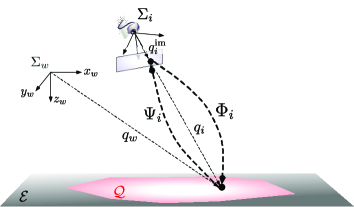
When a point on the environment with coordinates $q_{i}$ relative to $\Sigma_{i}$ is captured by a sensor $i$ with $g_{wi}$, the point is projected onto the image plane as illustrated in Fig. 4. If the coordinates of the projected point are denoted by $q_{i}^{\rm im}\in{\mathcal{F}}_{i}$, it is well known that the projection is formulated as

$$q_{i}^{\rm im}=\Psi_{i}(q_{i})=\frac{\lambda_{i}}{{\bf e}_{3}^{T}q_{i}}q_{i}.$$ (3)

It is not difficult to show that the inverse map $\Phi_{i}$ of the map $\Psi_{i}$ (Fig. 4) from $q^{\rm im}_{i}$ to $q_{i}$ is given by

$$q_{i}=\Phi_{i}(q^{\rm im}_{i})=\frac{\delta_{i}q^{\rm im}_{i}}{{\bf e}_{3}^{T}R_{wi}q^{\rm im}_{i}}.$$ (4)

Note that, while $\Psi_{i}$ is independent of $R_{wi}$, the map $\Phi_{i}$ depends on $R_{wi}$ and hence we describe $\Phi_{i}$ as $\Phi_{i}(q^{\rm im}_{i};R_{wi})$.

Figure 4: Projections $\Psi_{i}$ and $\Phi_{i}$.

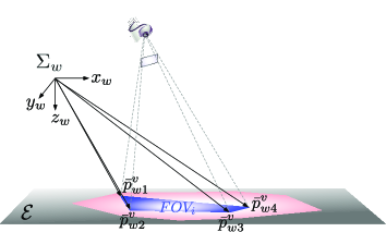
Using the map $\Phi_{i}$, we denote by $FOV_{i}(R_{wi})$ the set of coordinates of the field of view (FOV) of each sensor $i$ relative to $\Sigma_{w}$, which is also a polytope. Its ${\mathcal{V}}$-polytope representation is trivial, namely it is given by the convex hull of the four points with coordinates

$${q}^{v}_{wl}(R_{wi})=g_{wi}\circ\Phi_{i}(p^{v}_{il};R_{wi})$$ (5)

relative to $\Sigma_{w}$ (Fig. 5). The ${\mathcal{H}}$-polytope representation is also computed efficiently as follows.

Suppose now that $l$-th side line segment ($l=1,2,3,4$) specifying the boundary of the image plane connects the vertices $1$ and $2$ without loss of generality. Then, the line projected onto the environment is also a line segment whose vertices have coordinates ${p}^{v}_{w1}(R_{wi})$ and ${p}^{v}_{w2}(R_{wi})$ relative to $\Sigma_{w}$, and hence the line is formulated as

$$\left\{q\in{\mathcal{E}}\left|\ A^{i}_{l}(R_{wi})\begin{bmatrix}q_{1}\\ q_{2}\end{bmatrix}=1,\ q_{3}=\gamma\right.\right\},$$

where the matrix $A_{l}(R_{wi})\in{\mathbb{R}}^{2\times 2}$ is derived as

$$A^{i}_{l}(R_{wi})=\begin{bmatrix}1&1\end{bmatrix}\begin{bmatrix}\begin{bmatrix}{\bf e}_{1}^{T}\\ {\bf e}_{2}^{T}\end{bmatrix}{q}^{v}_{w1}(R_{wi})&\begin{bmatrix}{\bf e}_{1}^{T}\\ {\bf e}_{2}^{T}\end{bmatrix}{q}^{v}_{w2}(R_{wi})\end{bmatrix}^{-1}$$

from the fact that ${q}^{v}_{w1}(R_{wi})$ and ${q}^{v}_{w2}(R_{wi})$ are on the line. Since the coordinates $p_{w}^{0}=g_{wi}\circ\Phi_{i}(p_{i}^{0};R_{wi})$ for any interior $p_{i}^{0}$ of ${\mathcal{F}}_{i}$ must be inside the FOV, a half space specifying the FOV is described by the inequality $\bar{A}_{l}^{i}(R_{wi})q\leq\bar{a}_{l}^{i}(R_{wi})$ with

$$\bar{A}_{l}^{i}(R_{wi}):=\bar{a}_{l}^{i}(R_{wi})A_{l}^{i}(R_{wi}),\ \bar{a}_{l}^{i}:={\rm sign}(1-A_{l}^{i}(R_{wi})p_{w}^{0}).$$

In the same way, we can find the pair $\bar{A}_{l}^{i}(R_{wi}),\ \bar{a}_{l}^{i}$ for all $l=1,2,3,4$. Stacking them allows one to formulate the FOV as

$$FOV_{i}(R_{wi})=\left\{q\in{\mathcal{E}}\left|\ A^{i}(R_{wi})\begin{bmatrix}q_{1}\\ q_{2}\end{bmatrix}=a^{i}(R_{wi}),\ q_{3}=\gamma\right.\right\}.$$

III Coverage for a Single Sensor

In this section, we consider a simple case with ${\mathcal{V}}=\{i\}$.

III-A Objective Function

Let us first define the objective function to be minimized by sensor $i$. In this paper, we basically take the concept of coverage control [11, 12], where the objective function is defined by a sensing performance function and a density function at a point $q\in{\mathcal{E}}$. Note however that we accumulate the function only at the center of the pixels projected onto the environment ${\mathcal{E}}$ in order to reflect the discretized nature of the vision sensors. In the sequel, the sensing performance function and the density function at $q\in{\mathcal{E}}$ are denoted by $f_{i}(q):{\mathcal{E}}\to{\mathbb{R}}_{+}$ and $\phi(q):{\mathcal{E}}\to{\mathbb{R}}_{+}$, respectively.

Let us first define a function $q_{wl}(R_{wi}):SO(3)\to{\mathcal{E}}$ providing the coordinates in $\Sigma_{w}$ of the point on ${\mathcal{E}}$ which is captured by $l$-th pixel as

$$q_{wl}(R_{wi})\!\! \!\!=\!\! \!\!g_{wi}\circ\Phi_{i}(p_{il};R_{wi})=\frac{\delta_{i}R_{wi}p_{il}}{{\bf e}_{3}^{T}R_{wi}p_{il}}+p_{wi}.$$ (6)

Then, the objective function takes the form of

$$H_{i}(R_{wi})\!\! \!\!=\!\! \!\!\sum_{l\in{\cal L}_{i}}w_{il}(f_{i}\circ q_{wl}(R_{wi}))(\phi\circ q_{wl}(R_{wi})),$$ (7)

where $w_{il}>0$ is a weighting coefficient. If we impose a large $w_{il}$ on the pixel at around the center of the image, the sensor tends to capture the important area at around the image center. If we need to accelerate computation, replacing ${\cal L}_{i}$ in (7) by its subset is an option. In order to ensure preciseness, we need to introduce an extended function allowing $\pm\infty$, but we will not mention it since it can be easily avoided by choosing $f_{i}(q)$ appropriately.

Figure 5: Field of view $FOV_{i}$

Similarly to [12], we let the performance function $f_{i}(q)$ depend only on the distance $\|q-p_{wi}\|$. Remark however that, differently from [12], the third element of $q-p_{wi}$ is not controllable since the sensor is fixed. This may cause a problem that penalty of seeing distant area does not work in the case that the element is large enough. However, the element is not ignorable since it reflects heterogeneous characteristics of vision sensors in the multi-sensor case. We thus use the weighting distance as

$$f_{i}(q)=\frac{1}{\lambda_{i}}\|q-p_{wi}\|_{W}^{2}=\frac{1}{\lambda_{i}}(q-p_{wi})^{T}W(q-p_{wi}).$$ (8)

with $W\geq 0$, where $1/\lambda_{i}$ is introduced since the distance is scaled by the focal length. Suppose that $W$ is set as $W={\rm diag}([w\ w\ 1])$. Then, a large $w$ imposes a heavy penalty on viewing distant area and a small $w$ a light penalty on it. In particular, when $q=q_{wl}(R_{wi})$ for some $l\in{\cal L}_{i}$, (8) is rewritten as

$$f_{i}\circ q_{wl}(R_{wi})=\frac{\tilde{\delta}_{i}\|R_{wi}p_{il}\|_{W}^{2}}{\|{\bf e}_{3}^{T}R_{wi}p_{il}\|^{2}},\ \ \tilde{\delta}_{i}=\frac{\delta_{i}^{2}}{\lambda_{i}}.$$ (9)

Once the density function $\phi$ is given, the goal is reduced to minimization of (7) with (9) under the restriction of $R_{wi}\in SO(3)$. In order to solve the problem, this paper takes the gradient descent approach which is a standard approach to coverage control. For this purpose, it is convenient to define an extension $\bar{H}_{i}:{\mathbb{R}}^{3\times 3}\to{\mathbb{R}}_{+}$ such that $\bar{H}_{i}(M)=H_{i}$ if $M\in SO(3)$. We first extend the domain of $q_{wl}(\cdot)$ in (6) from $SO(3)$ to ${\mathbb{R}}^{3\times 3}$ as

$$\bar{q}_{wl}(M)=\frac{\delta_{i}Mp_{il}}{{\bf e}_{3}^{T}Mp_{il}}+p_{wi}.$$ (10)

Then, the vector $\bar{q}_{wl}(M)\in{\mathbb{R}}^{3}$ is not always on the environment when $M\notin SO(3)$ but the function $f_{i}$ in (8) is well-defined even if the domain is altered from ${\mathcal{E}}$ to ${\mathbb{R}}^{3}$. We thus denote the function with the domain ${\mathbb{R}}^{3}$ by $\bar{f}_{i}$, and define the composite function

$$\bar{f}_{i}\circ\bar{q}_{wl}(M)=\frac{\tilde{\delta}_{i}\|Mp_{il}\|_{W}^{2}}{\|{\bf e}_{3}^{T}Mp_{il}\|^{2}}.$$ (11)

Figure 6: Coordinates of $q\in{\mathcal{E}}$ relative to $\Sigma_{w}$ and $\Sigma_{i}$.

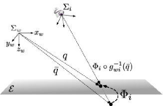
We next focus on the term $\phi\circ q_{wl}(R_{wi})$ in (7) and expand the domain of the composite function from $SO(3)$ to ${\mathbb{R}}^{3\times 3}$. Here, since $\bar{q}_{wl}(M)$ is not always on ${\mathcal{E}}$, we need to design $\bar{\phi}:{\mathbb{R}}^{3}\to{\mathbb{R}}_{+}$ such that $\bar{\phi}(q)=\phi(q)$ if $q\in{\mathcal{E}}$. In this paper, we assign to a point $\bar{q}\in{\mathbb{R}}^{3}$ the density of a point

$$q=g_{wi}\circ\Phi\circ g_{wi}^{-1}(\bar{q})=\frac{\delta_{i}(\bar{q}-p_{wi})}{{\bf e}_{3}^{T}(\bar{q}-p)}+p_{wi},$$

where the operations are illustrated in Fig. 6. Accordingly, the density function is defined by

$$\bar{\phi}(\bar{q})=\phi\circ g_{wi}\circ\Phi\circ g_{wi}^{-1}(\bar{q}).$$ (12)

Remark that, differently from $f_{i}$, the function $\phi$ is not naturally extended and the selection of $\bar{\phi}$ is not unique. The motivation to choose (12) will be clear in the next subsection.

Consequently, we define the extended objective function

$$\bar{H}_{i}(M)\!\! \!\!=\!\! \!\!\sum_{l\in{\cal L}_{i}}w_{il}(\bar{f}_{i}\circ\bar{q}_{wl}(M))(\bar{\phi}\circ\bar{q}_{wl}(M)),$$ (13)

from ${\mathbb{R}}^{3\times 3}$ to ${\mathbb{R}}_{+}$ by using (11) and (12). Let us finally emphasize that $H_{i}(M)=\bar{H}_{i}(M)$ holds for any $M\in SO(3)$.

III-B Density Estimation for Moving Objects Monitoring

In the gradient descent approach, we update the rotation $R_{wi}$ in the direction of ${\rm grad}_{R_{wi}[k]}^{SO(3)}H_{i}$ at each time $k$. This subsection assumes that the density $\phi$ is not given a priori and that $\phi$ needs to be estimated from acquired vision data as investigated in [4, 14].

Let us first consider an ideal situation such that the density function is exactly projected onto the image plane, namely

$$\phi(q)=\psi\circ\Psi_{i}\circ g_{wi}^{-1}[k](q)\ {\forall q}\in FOV_{i}(R_{wi}[k]),$$ (14)

holds with respect to the density $\psi:{\mathcal{F}}_{i}\to{\mathbb{R}}_{+}$ over the image plane. Then, the density function value $\phi(q)$ is available at any point in the FOV. We next consider a point $\bar{q}\in{\mathbb{R}}^{3}$ which does not always lie on ${\mathcal{E}}$. Then, the value of $\bar{\phi}(\bar{q})$ is also given by the same function as (14) since

$$\bar{\phi}(\bar{q})\!\! \!\!=\!\! \!\!\phi\circ g_{wi}[k]\circ\Phi\circ g_{wi}^{-1}[k](\bar{q})$$

$$\!\!=\!\! \!\!\psi\circ\Psi_{i}\circ g_{wi}^{-1}[k]\circ g_{wi}[k]\circ\Phi\circ g_{wi}^{-1}[k](\bar{q})$$

$$\!\!=\!\! \!\!\psi\circ\Psi_{i}\circ\Phi\circ g_{wi}^{-1}[k](\bar{q})=\psi\circ\Psi_{i}\circ g_{wi}^{-1}[k](\bar{q}).$$

Ensuring the equality is the reason for choosing (12).

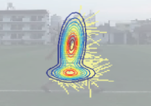
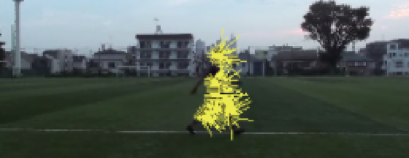
Figure 7: A snapshot and computed optical flows.

We next consider estimation of the density $\psi$ on the image since assuming (14) is unrealistic. Rich literature has been devoted to the information extraction from the raw vision data, and a variety of algorithms are currently available even without expert knowledge [17]. For example, it is possible to detect and localize in the image plane specific objects like cars or human faces, and even abstract targets such as everything moving or some environmental changes.

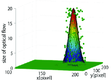
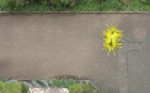
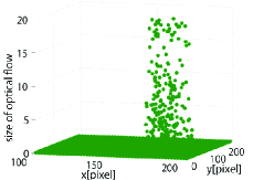
The present coverage scheme is indeed applicable to any scenario such that a nonnegative number $y_{il}$ reflecting its own importance is assigned to each pixel $l\in{\cal L}_{i}$ after conducting some image processing. However, we mainly focus on a specific scenario of monitoring moving objects on the mission space. Suppose that a sensor captures a human walking from left to right in the image as in Fig. 7. Then, a way to localize such moving objects is to compute optical flows from consecutive images as in Fig. 7, where the flows are depicted by yellow lines. We also let the data $y_{il}$ be the norm of the flow vector at each pixel. Then, the plots of $y_{il}$ over the image plane are illustrated by green dots in Fig. 9.

Figure 8: Plots of $y_{il}$.

Figure 9: Estimated density.

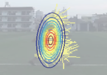
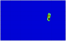
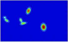
We next fit the data of $y_{il}$ by a continuous function defined over ${\mathcal{F}}_{i}$ and use the function as $\psi$. Such algorithms are also available even in real time [18]. Similarly to [14], we employ the mixed Gaussian function known to approximate a variety of functions with excellent precision by increasing the number of Gaussian functions, and widely used in data mining, pattern recognition, machine learning and statistical analysis. Fig. 9 shows the Gaussian function with $m=1$ computed so as to fit the data in Fig. 9. Of course, using a larger $m$ achieves a better approximation as shown in Fig. 10.

As a result, we obtain a function in the form of

$$\sum_{j=1}^{m}\alpha_{j}e^{-\|p^{\rm im}-\mu^{\rm im}_{j}\|^{2}_{\Sigma_{j}^{\rm im}}},\ \ \Sigma_{j}^{\rm im}>0$$ (15)

over the 2-D image plane coordinates $p^{\rm im}\in{\mathbb{R}}^{2}$. Note that (15) is large when $p^{\rm im}$ captures an important point, which is opposite to the density function. Thus, we define the function

$$\psi^{\rm im}(p^{\rm im})=\bar{\psi}-\sum_{j=1}^{m}\alpha_{j}e^{-\|p^{\rm im}-\mu^{\rm im}_{j}\|^{2}_{\Sigma_{j}^{\rm im}}},$$ (16)

where $\bar{\psi}<\bar{\phi}$ is a positive scalar guaranteeing $\psi^{\rm im}(p^{\rm im})\geq 0$ for all $p^{\rm im}$. It is also convenient to define $\psi(p)$ for all 3-D vectors $p\in{\mathcal{F}}_{i}$ on the image plane as

$$\psi(p)\!\! \!\!=\!\! \!\!\left\{\begin{array}[]{l}\bar{\phi},\ \mbox{if }g_{wi}\circ\Phi_{i}(p)\notin{\mathcal{Q}}\\ \bar{\psi}-\sum_{j=1}^{m}\alpha_{j}e^{-\|p-\mu_{j}\|^{2}_{\Sigma_{j}}},\ \mbox{otherwise}\end{array}\right.,$$ (19)

$$\mu_{j}\!\! \!\!=\!\! \!\!\begin{bmatrix}\mu^{\rm im}_{j}\\ \lambda_{i}\end{bmatrix},\ \ \Sigma_{j}=\begin{bmatrix}\Sigma_{j}^{\rm im}&0\\ 0&0\end{bmatrix}.$$ (20)

Figure 10: Estimated densities for $m=1$(left) and $m=2$(right).

III-C Gradient Computation

Full 3-D Rotational Motion

Here, we will derive the gradient ${\rm grad}_{R_{wi}[k]}^{SO(3)}H_{i}$, given a rotation $R_{wi}[k]\in SO(3)$ and $\psi$ in (19). It is widely known that $T_{R_{wi}}SO(3)$ is formulated as $T_{R_{wi}}SO(3)=\{R_{wi}X\in{\mathbb{R}}^{3\times 3}|\ X\in so(3)\}$, where $so(3)$ is the set of all skew symmetric matrices in ${\mathbb{R}}^{3\times 3}$. We also define the operator $\wedge$(wedge) from ${\mathbb{R}}^{3}$ to ${\mathbb{R}}^{3\times 3}$ such that $a\times b=\hat{a}b$ for the cross product $\times$. The rotational group $SO(3)$ is known to be a submanifold of a Riemannian manifold ${\mathbb{R}}^{3\times 3}$ with $T_{x}{\mathbb{R}}^{3\times 3}={\mathbb{R}}^{3\times 3}\supset T_{R_{wi}}SO(3)$ and the Riemannian metric

$$\langle M,N\rangle={\rm tr}(M^{T}N),\ M,N\in{\mathbb{R}}^{3\times 3}$$ (21)

[16]. It is also known that the orthogonal projection $P_{R_{wi}}$ of matrix $M\in T_{R_{wi}}{\mathbb{R}}^{3\times 3}={\mathbb{R}}^{3\times 3}$ onto $T_{R_{wi}}SO(3)$ in terms of the Riemannian metric induced by (21) is given by

$$P_{R_{wi}}(M)=R_{wi}{\rm sk}(R_{wi}^{T}M),\ \ {\rm sk}(M)=\frac{1}{2}(M-M^{T}).$$ (22)

See Subsection 3.6.1 of [16] for more details.

Now, we have the following theorem, where we use the notation $\tilde{\cal L}_{i}(R_{wi})=\{l\in{\cal L}_{i}|\ g_{wi}\circ\Phi(p_{il};R_{wi})\in{\mathcal{Q}}\}$ and $\tilde{\cal L}_{i}^{c}(R_{wi})={\cal L}_{i}\setminus\tilde{\cal L}_{i}(R_{wi})$.

Theorem 1

Suppose that the objective function $\bar{H}_{i}$ is formulated by (13) with (11), (12) and (19). Then, the gradient ${\rm grad}_{R_{wi}[k]}^{SO(3)}H_{i}$ is given by

$${\rm grad}_{R_{wi}[k]}^{SO(3)}H_{i}\!\! \!\!=\!\! \!\!P_{R_{wi}[k]}\left({\rm grad}_{R_{wi}[k]}^{{\mathbb{R}}^{3\times 3}}\bar{H}_{i}\right),$$ (23)

$${\rm grad}_{R_{wi}[k]}^{{\mathbb{R}}^{3\times 3}}\bar{H}_{i}\!\! \!\!=\!\! \!\!\tilde{\delta}_{i}\eta_{i}^{T}(R_{wi}[k])p_{il}^{T},$$

where

$$\eta_{i}(R)\!\! \!\!=\!\! \!\!\!\!\sum_{l\in\tilde{\cal L}_{i}^{c}(R)}w_{il}\bar{\phi}\eta_{i}^{l}+\!\!\sum_{l\in\tilde{\cal L}_{i}(R)}\!\!w_{il}\Big{(}\bar{\psi}\eta_{i}^{l}-\sum_{j=1}^{m}\alpha_{j}\eta_{i}^{lj}\Big{)}$$

$$\tilde{\cal L}_{i}(R)\!\! \!\!=\!\! \!\!\{l\in{\cal L}_{i}|\ q_{wl}(R)\in{\mathcal{Q}}\},\ \tilde{\cal L}_{i}^{c}(R)={\cal L}_{i}\setminus\tilde{\cal L}_{i}(R)$$

$$\eta_{i}^{l}(R)\!\! \!\!=\!\! \!\!\frac{2}{({\bf e}_{3}^{T}Rp_{il})^{3}}\Big{(}({\bf e}_{3}^{T}Rp_{il})p_{il}^{T}R^{T}W-\|Rp_{il}\|_{W}^{2}{\bf e}_{3}^{T}\Big{)}$$

$$\eta_{i}^{lj}(R)\!\! \!\!=\!\! \!\!\frac{2e^{-\|b_{lj}\|^{2}_{\Sigma_{j}}}}{\lambda_{i}({\bf e}_{3}^{T}Rp_{il})^{3}}\Big{(}({\bf e}_{3}^{T}Rp_{il})\xi^{lj}_{i}(R)-\lambda_{i}\|Rp_{il}\|_{W}^{2}{\bf e}_{3}^{T}\Big{)}$$

$$\xi^{lj}_{i}(R)\!\! \!\!=\!\! \!\!\|Rp_{il}\|_{W}^{2}b_{lj}^{T}\Sigma_{j}(p_{il}{\bf e}_{3}^{T}-\lambda_{i}I_{3})R^{T}+\lambda_{i}p_{il}^{T}R^{T}W$$

Proof:

See Appendix A. ∎

Namely, just running the dynamics

$$\dot{R}_{wi}=-K{\rm grad}_{R_{wi}}^{SO(3)}H_{i},\ K>0$$ (24)

leads $R_{wi}$ to the set of critical points of $H_{i}$. However, in practice, the vision data is usually obtained at discrete time instants and hence we approximate the continuous-time algorithm (24) by

$${R}_{wi}[k+1]=R_{wi}[k]{\rm exp}\left(R_{wi}^{T}[k]\left(\alpha_{k}{\rm grad}_{R_{wi}[k]}^{SO(3)}H_{i}\right)\right).$$ (25)

See [16] for the details on the selection of $\alpha_{k}$.

Rotational Motion with Underactuations

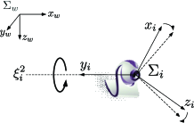
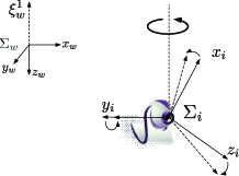
Figure 11: Pan motion.

Figure 12: Tilt motion.

In the above discussion, we assume that the sensor can take full 3-D rotational motion. However, the motion of many commoditized cameras is restricted by the actuator configurations. Hereafter, we suppose that the sensor can be rotated around two axes $\xi^{1}_{i}$ ($\|\xi^{1}_{i}\|=1$) and $\xi_{i}^{2}$ ($\|\xi^{2}_{i}\|=1$), where these vectors are defined in $\Sigma_{i}$ and assumed to be linearly independent of each other. These axes may depend on the rotation matrix $R_{wi}$. For example, in the case of Pan-Tilt (PT) cameras in Figs. 12 and 12, which are typical commoditized cameras, the axis of the pan motion (Fig. 12) is fixed relative to $\Sigma_{w}$, while that of the tilt motion (Fig. 12) is fixed relative to the sensor frame $\Sigma_{i}$. Then, only one of the two axes depends on $R_{wi}$. Note that even when there is only one axis around which the sensor can be rotated, the subsequent discussions are valid just letting $\xi_{i}^{2}=0$.

Let us denote a normalized vector $\xi^{3}_{i}$ ($\|\xi_{1}^{3}\|=1$) orthogonal to the $\xi^{1}_{i},\xi^{2}_{i}$-plane. Then, the three vectors $\xi^{1}_{i}$, $\xi^{2}_{i}$ and $\xi_{i}^{3}$ span ${\mathbb{R}}^{3}$. Thus, any element $\Theta$ of $T_{R_{wi}}SO(3)$ can be represented in the form of $\Theta=R_{wi}\sum_{j=1}^{3}\beta_{j}\hat{\xi}_{i}^{j},\ \ \beta_{j}\in{\mathbb{R}}$. Now, we define a distribution $\Delta$ [19] assigning $R_{wi}\in SO(3)$ to the subspace

$$\left\{\Theta\in T_{R_{wi}}SO(3)\left|\ \Theta=R_{wi}\sum_{j=1}^{2}\beta_{j}\hat{\xi}_{i}^{j},\ \beta_{1},\beta_{2}\in{\mathbb{R}}\right.\right\},$$ (26)

whose dimension is $2$. The distribution $\Delta$ is clearly regular and hence induces a submanifold ${\mathcal{S}}_{UA}$ of $SO(3)$ [19], called integral manifold, such that its tangent space $T_{R_{wi}}{\mathcal{S}}_{UA}$ at $R_{wi}\in{\mathcal{S}}_{UA}\subseteq SO(3)$ is equal to (26). The manifold ${\mathcal{S}}_{UA}$ specifies orientations which the camera can take.

Since ${\mathcal{S}}_{UA}$ is a submanifold of $SO(3)$, a strategy similar to Theorem 1 is available and we have the following corollary.

Corollary 1

Suppose that the objective function $\bar{H}_{i}$ is formulated by (13) with (11), (12) and (19). Then, the gradient ${\rm grad}_{R_{wi}[k]}^{{\mathcal{S}}_{UA}}H_{i}$ is given by

$${\rm grad}_{R_{wi}[k]}^{{\mathcal{S}}_{UA}}H_{i}\!\! \!\!=\!\! \!\!P^{UA}_{R_{wi}[k]}\left({\rm grad}_{R_{wi}[k]}^{SO(3)}H_{i}\right)$$ (27)

where the orthogonal projection $P^{UA}_{R_{wi}}(M)$ of $M=R_{wi}N\in T_{R_{wi}}SO(3),\ N\in so(3)$ to $T_{R_{wi}}{\mathcal{S}}_{UA}$ is defined by

$$P^{UA}_{R_{wi}}(M)\!\! \!\!=\!\! \!\!R_{wi}(\alpha_{1}\hat{\xi}_{i}^{1}+\alpha_{2}\hat{\xi}_{i}^{2})$$ (28)

with $\alpha_{l}=\frac{\langle N,\hat{\xi}_{i}^{l}\rangle-\langle\hat{\xi}_{i}^{1},\hat{\xi}_{i}^{2}\rangle\langle N,\hat{\xi}_{i}^{-l}\rangle}{1-\langle\hat{\xi}_{i}^{1},\hat{\xi}_{i}^{2}\rangle^{2}}$ $l=1,2$, where $-l=2$ if $l=1$ and $-l=1$ if $l=2$.

We see from this corollary that the gradient ${\rm grad}_{R_{wi}[k]}^{SO(3)}H_{i}$ on $SO(3)$ is utilized as it is and we need only to project it through (28). Also, the projection (28) is successfully parameterized by the vectors $\xi_{i}^{1}$ and $\xi_{i}^{2}$.

IV Coverage for Multiple Sensors

Figure 13: Overlaps of FOVs (green region).

In this section, we extend the result of the previous section to the multi-sensor case. The difference from the single sensor case stems from the overlaps of the FOVs with the other sensors as illustrated in Fig. 13. [4, 11, 13] present sensing performance functions taking account of the overlaps and their gradient decent laws. However, in this paper, we present another simpler scheme to manage the overlap.

Let us first define the set of sensors capturing a point $q\in{\mathcal{E}}$ within the FOV as ${\mathcal{V}}(q;R_{{\mathcal{V}}})=\{i\in{\mathcal{V}}|\ q\in FOV_{i}(R_{wi})\}$ where $R_{{\mathcal{V}}}=(R_{wi})_{i\in{\mathcal{V}}}$. We also suppose that, when ${\mathcal{V}}(q;R_{{\mathcal{V}}})$ has multiple elements for some $q\in Q$, only the data of the sensor with the minimal sensing performance (8) among sensors in ${\mathcal{V}}(q;R_{{\mathcal{V}}})$ is employed in higher-level decisions and recognitions. This motivates us to partition $FOV_{i}(R_{wi})$ into the two region

$$SFOV_{i}(R_{{\mathcal{V}}})\!\! \!\!=\!\! \!\!\{q\in FOV_{i}(R_{wi})|\ i\in\arg\min_{j\in{\mathcal{V}}(q;R_{{\mathcal{V}}})}f_{j}(q)\},$$

$$SFOV^{c}_{i}(R_{{\mathcal{V}}})\!\! \!\!=\!\! \!\!\{q\in FOV_{i}(R_{wi})|\ i\notin\arg\min_{j\in{\mathcal{V}}(q;R_{{\mathcal{V}}})}f_{j}(q)\}.$$

Then, what pixel $l$ captures a point in $SFOV^{c}_{i}(R_{{\mathcal{V}}})$ is identified with what it captures a point outside of ${\mathcal{Q}}$, whose cost is set as $\bar{\phi}(f_{i}\circ q_{w})$ in the previous section, in the sense that both of the data are not useful at all. This is reflected by assigning $\bar{\phi}$ to the pixels $l\notin\tilde{\cal L}_{i}(R_{{\mathcal{V}}})$ with $\tilde{\cal L}_{i}(R_{{\mathcal{V}}})=\{l\in{\cal L}_{i}|\ q_{wl}(R_{wi})\in SFOV_{i}(R_{{\mathcal{V}}})\cap{\mathcal{Q}}\}$.

Accordingly, we formulate the function to be minimized by ${\mathcal{V}}$ as $H(R_{{\mathcal{V}}})=\sum_{i\in{\mathcal{V}}}H_{i}(R_{{\mathcal{V}}})$ with

$$H_{i}(R_{{\mathcal{V}}})\!\! \!\!=\!\! \!\!\sum_{l\in\tilde{\cal L}_{i}(R_{{\mathcal{V}}})}w_{il}(f_{i}\circ q_{wl}(R_{wi}))(\phi\circ q_{wl}(R_{wi}))$$ (29)

$$\hskip 28.45274pt+\bar{\phi}\sum_{l\notin\tilde{\cal L}_{i}(R_{{\mathcal{V}}})}w_{il}f_{i}\circ q_{wl}(R_{wi}).$$

Remark that (29) differs from (7) only in the set $\tilde{\cal L}_{i}(R_{{\mathcal{V}}})$.

Strictly speaking, to compute the gradient of (29), we need to expand ${\cal L}_{i}(R_{{\mathcal{V}}})$ from $SO(3)\times\cdots\times SO(3)$ to ${\mathbb{R}}^{3\times 3}\times\cdots\times{\mathbb{R}}^{3\times 3}$. For this purpose, it is sufficient to define $\bar{FOV}_{i}(M)$ from ${\mathbb{R}}^{3\times 3}$ to a subset of ${\mathcal{E}}$. For example, an option is to define an extension

$$\bar{q}^{v}_{wl}(M)=\frac{\delta_{i}Mp^{v}_{il}}{{\bf e}_{3}^{T}Mp^{v}_{il}}+p_{wi},\ l=1,2,3,4.$$ (30)

of (5) similarly to (10), and to let $\bar{FOV}_{i}(M)$ be the convex full of these points. However, at the time instants computing the gradient with $R_{{\mathcal{V}}}[k]$, the extension $\bar{\cal L}_{i}(M_{{\mathcal{V}}})$ for a sufficiently small perturbation $M_{{\mathcal{V}}}-R_{{\mathcal{V}}}$ is equivalent to the original set $\tilde{\cal L}_{i}(R_{{\mathcal{V}}})$ irrespective of the selection of $\bar{FOV}_{i}(M)$ except for the pathological case when a pixel is located on the boundary of $SFOV_{i}(R_{{\mathcal{V}}})$. Namely, ignoring such pathological cases which do not happen almost surely for (25), the gradient can be computed by using the set $\tilde{\cal L}_{i}(R_{{\mathcal{V}}}[k])$ instead of its extension. Hence, the gradient is simply given as Theorem 1 by just replacing $\tilde{\cal L}_{i}(R_{wi})$ by $\tilde{\cal L}_{i}(R_{{\mathcal{V}}})$. Note that the curve fitting process is run without taking account of whether $l\in\tilde{\cal L}_{i}(R_{wi})$ or not, and $\bar{\phi}$ is assigned to $l\notin\tilde{\cal L}_{i}(R_{wi})$ at the formulation of $\psi$ as in (19). This is because letting $y_{il}=0\ {\forall l}\notin\tilde{\cal L}_{i}(R_{wi})$ at the curve fitting stage would degrade the density estimation accuracy at around the boundary of $SFOV_{i}$.

The remaining issue is efficient computation of the set $\tilde{\cal L}_{i}(R_{wi})$. Hereafter, we assume that each sensor acquires $FOV_{j}\ {\forall j}\in{\mathcal{V}}\setminus\{i\}$, i.e. $\bar{A}_{i}^{l}(R_{wj})$ and $\bar{a}_{i}^{l}(R_{wj})$ for all $l=1,2,3,4$, and its index $j$ through (all-to-all) communication or with the help of a centralized computer. The computation under the limited communication will be mentioned at the end of this section. In addition, we suppose that every sensor stores the set

$${\mathcal{Q}}_{ij}=\left\{q\in{\mathcal{Q}}\left|\ \lambda_{j}\left\|q-p_{wi}\right\|_{W}^{2}>\lambda_{i}\left\|q-p_{wj}\right\|_{W}^{2}\right.\right\},$$ (31)

for all $j\in{\mathcal{V}}$ which can be computed off-line since the sensor positions are fixed.

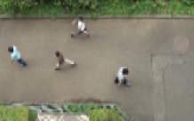
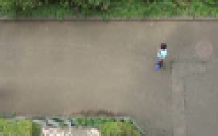
Figure 14: Images at $t=0$s (left) and $t=4$s (right).

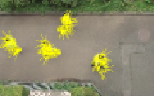
Figure 15: Optical flows of images at $t=0$s (left) and $t=4$s (right).

Figure 16: Approximation of data at $t=0$s (left) and $t=4$s (right).

Then, the set $SFOV^{c}_{i}(R_{{\mathcal{V}}})$ is computed as

$$SFOV^{c}_{i}(R_{{\mathcal{V}}})=\bigcup_{j\in{\mathcal{V}}\setminus\{i\}}({\mathcal{Q}}_{ij}\cap FOV_{i}\cap FOV_{j}).$$ (32)

in polynomial time with respect to $n$. Namely, checking $q_{wl}(R_{wi})\in SFOV^{c}_{i}(R_{{\mathcal{V}}})$ for all $l\in{\cal L}_{i}$ provides $\tilde{\cal L}_{i}(R_{{\mathcal{V}}})$.

The computation process including image processing, curve fitting and gradient computation is successfully distributed to each sensor but the resulting FOVs need to be shared among all sensors to compute $\tilde{\cal L}_{i}(R_{{\mathcal{V}}})$. A way to implement the present scheme under limited communication is to restrict the FOV of each sensor so that the FOV can overlap with limited number of FOVs of the other sensors. Such constraints on the FOVs are easily imposed by adding an artificial potential to the objective function but we leave the issue as a future work due to the page constraints.

V Simulation of Moving Objects Monitoring

In this section, we demonstrate the utility of the present approach through simulation using 4 cameras with $\lambda_{i}=3.4$mm ${\forall i}$. Here, we suppose that the view of the environment from $\Sigma_{w}$ with $\gamma=10$m and focal length $3.4$mm is given as in Fig. 16, and that the mission space ${\mathcal{Q}}$ is equal to the FOV corresponding to the image. Since the codes of simulating the image acquisition and processing are never used in experiments, we simplify the process as follows, and demonstrate only the present coverage control scheme with the curve fitting process. Before running the simulation, we compute the optical flows for the images of Fig. 16 as in Fig. 16, and also fitting functions of the data as in Fig. 16. The resulting data is uploaded at http://www.fl.ctrl.titech.ac.jp/paper/2014/data.wmv. Then, we segment the image by the superlevel set of the function using a threshold $10^{-3}$, and assign a boolean variable $1$ to $y_{il}$ if $q_{wl}(R_{wi})$ is inside of the set and assign $0$ otherwise. The experimental system is now under construction, and the experimental verification of the total process will be conducted in a future work. Note however that it is at least confirmed that the skipped image acquisition and processing can be implemented within several milliseconds in a real vision system.

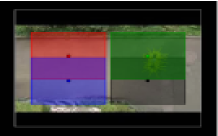
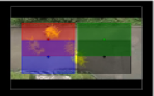
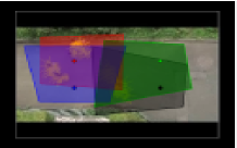
Figure 17: Initial FOVs (left) and final FOVs (right).

Figure 18: Evolution of objective function $H$.

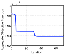
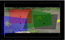
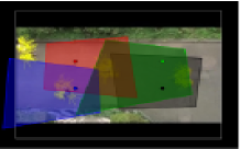
Let the position vectors of cameras be selected as $e_{3}^{T}p_{wi}=6\mbox{m},\ {\forall i}$ and the length of each side of the image plane be $6.4$mm and $4.8$mm. The other elements of $p_{wi}$ are set as illustrated by the mark $\bullet$ in Fig. 18. The parameters in $H$ is set as $\bar{\psi}=1$, $\bar{\phi}=1.05$, $w_{il}=\frac{\|p^{v}_{i1}\|+4\times 10^{-4}}{\|p_{il}\|+4\times 10^{-4}}$ and $W={\rm diag}([0.01\ 0.01\ 1])$. The curve fitting process is run with $m=3$ and the gradient is computed by evaluating the objective function not at all points in ${\cal L}_{i}$ but at 121 points extracted from ${\cal L}_{i}$. In order to confirm convergence of the orientations, we first fix the image as in Fig. 18 and run the present algorithm from the initial condition $R_{wi}=I_{3}\ {\forall i}$. Then, the evolution of the function $H$ is illustrated in Fig. 18, where we compute the value using not the individually estimated density but the data as in Fig. 16. We see from the figure that the function $H$ is decreasing through the update process and eventually reaches a stationary point. The final configuration is depicted in the right figure of Fig. 18. We next start to play the above movie and check adaptability to environmental changes, where the orientations are assumed to be updated at each frame. Then, the evolution of FOVs are shown in http://www.fl.ctrl.titech.ac.jp/paper/2014/sim.wmv whose snapshots at times $t=0,1,2,4$ are depicted in Fig. 19. We see from the movie and figures that the cameras adjust their rotations so as to capture moving humans. The above results show the effectiveness of the present approach.

VI Conclusions

In this paper, we have investigated visual coverage control where the vision sensors are assumed to be distributed over the 3-D space to monitor the 2-D environment and to be able to control their orientations. We first have formulated the problem as an optimization problem on $SO(3)$. Then, in order to solve the problem, we have presented the entire process including not only the gradient computation but also image processing and curve fitting, which are required to estimate the density function from the acquired vision data. Finally, we have demonstrated the effectiveness of the approach through simulation of moving objects monitoring.

Appendix A Proof of Theorem 1

For notational simplicity, we describe $R_{wi}[k]$ by $R$ in the sequel. Substituting (11), (12) and (19) into (13), the objective function to be minimized is formulated as

$$\!\!\!\!\!\bar{H}_{i}(M)\!\! \!\!=\!\! \!\!\tilde{\delta}_{i}\bar{\phi}\!\!\sum_{l\in\tilde{\cal L}_{i}^{c}}\!\!w_{il}H_{i}^{l}+\tilde{\delta}_{i}\!\!\sum_{l\in\tilde{\cal L}_{i}}\!\!w_{il}\Big{(}\bar{\psi}H_{i}^{l}-\!\!\sum_{j=1}^{m}\!\!\alpha_{j}H_{i}^{lj}\Big{)},$$ (33)

$$\!\!\!\!\!H_{i}^{l}(M)\!\! \!\!=\!\! \!\!\frac{\|Mp_{il}\|_{W}^{2}}{\|{\bf e}_{3}^{T}Mp_{il}\|^{2}},\ H_{i}^{lj}(M)=\frac{\|Mp_{il}\|_{W}^{2}}{\|{\bf e}_{3}^{T}Mp_{il}\|^{2}}E_{i}^{lj}(M),$$

$$\!\!\!\!\!E_{i}^{lj}(M)\!\! \!\!=\!\! \!\!\exp\left\{-\left\|\frac{\lambda_{i}R^{T}Mp_{il}}{{\bf e}_{3}^{T}R^{T}Mp_{il}}-\mu_{j}\right\|^{2}_{\Sigma_{j}}\right\}.$$

Figure 19: Snapshots at $t=0$s (top-left), $t=1$s (top-right), $t=2$s (bottom-left) and $t=4$s (bottom-right).

From Lemma 1 and the fact that $SO(3)$ is a submanifold of ${\mathbb{R}}^{3\times 3}$, we first compute the gradient ${\rm grad}_{R}^{{\mathbb{R}}^{3\times 3}}\bar{H}_{i}(R)$. From Definition 1 and (1), we need to compute the directional derivative $D\bar{H}_{i}(R)[\Xi]$. From linearity of the directional derivative operator $D$, it is sufficient to derive $DH_{i}^{l}(R)[\Xi]$ and $DH_{i}^{lj}(R)[\Xi]$.

We first consider $DH_{i}^{l}(R)[\Xi]$. By calculation, we have

$$\tilde{H}^{l}_{i}(R+\Xi t)-\tilde{H}^{l}_{i}(R)=\frac{\|(R+\Xi t)p_{il}\|_{W}^{2}}{\|{\bf e}_{3}^{T}(R+\Xi t)p_{il}\|^{2}}-\frac{\bar{\psi}\|Rp_{il}\|_{W}^{2}}{\|{\bf e}_{3}^{T}Rp_{il}\|^{2}}$$

$$\hskip 5.69046pt=\frac{\|{\bf e}_{3}^{T}Rp_{il}\|^{2}\|(R+\Xi t)p_{il}\|_{W}^{2}}{\|{\bf e}_{3}^{T}(R+\Xi t)p_{il}\|^{2}\|{\bf e}_{3}^{T}Rp_{il}\|^{2}}$$

$$\hskip 91.04872pt-\frac{\|{\bf e}_{3}^{T}(R+\Xi t)p_{il}\|^{2}\|Rp_{il}\|_{W}^{2}}{\|{\bf e}_{3}^{T}(R+\Xi t)p_{il}\|^{2}\|{\bf e}_{3}^{T}Rp_{il}\|^{2}}$$

$$\hskip 5.69046pt=2t\frac{({\bf e}_{3}^{T}Rp_{il})(p_{il}^{T}R^{T}W\Xi p_{il})-\|Rp_{il}\|_{W}^{2}({\bf e}_{3}^{T}\Xi p_{il})+o(t)}{\|{\bf e}_{3}^{T}(R+\Xi t)p_{il}\|^{2}({\bf e}_{3}^{T}Rp_{il})}$$

Hence, $DH_{i}^{l}(R)[\Xi]=\lim_{t\to 0}\frac{\tilde{H}^{l}_{i}(R+\Xi t)-\tilde{H}^{l}_{i}(R)}{t}$ is given by

$$DH_{i}^{l}(M)[\Xi]\!\! \!\!=\!\! \!\!\tilde{\eta}_{i}^{l}(R)\Xi p_{il},$$ (34)

$$\eta_{i}^{l}(R)\!\! \!\!=\!\! \!\!\frac{2(({\bf e}_{3}^{T}Rp_{il})p_{il}^{T}R^{T}W-\|Rp_{il}\|_{W}^{2}{\bf e}_{3}^{T})}{({\bf e}_{3}^{T}Rp_{il})^{3}}.$$

Let us next consider $D\bar{H}_{i}^{lj}(R)[\Xi]$. We first have the equations

$$\bar{H}^{lj}_{i}(R+\Xi t)=\frac{\|(R+\Xi t)p_{il}\|_{W}^{2}E^{lj}_{i}(R+\Xi t)}{\|{\bf e}_{3}^{T}(R+\Xi t)p_{il}\|^{2}}$$

$$\hskip 8.5359pt=\frac{(\|Rp_{il}\|_{W}^{2}+2tp_{il}^{T}R^{T}W\Xi p_{il}+o(t^{2}))E^{lj}_{i}(R+\Xi t)}{\|{\bf e}_{3}^{T}Rp_{il}\|^{2}+2t({\bf e}_{3}^{T}Rp_{il})({\bf e}_{3}^{T}\Xi p_{il})+t^{2}\|{\bf e}_{3}^{T}\Xi p_{il}\|^{2}.}$$

Hence, we also have

$$\bar{H}^{lj}_{i}(R+\Xi t)-\bar{H}^{lj}_{i}(R)$$

$$=\frac{(\|Rp_{il}\|_{W}^{2}+2tp_{il}^{T}R^{T}W\Xi p_{il}+o(t^{2}))E^{lj}_{i}(R+\Xi t)}{\|{\bf e}_{3}^{T}Rp_{il}\|^{2}+2t({\bf e}_{3}^{T}Rp_{il})({\bf e}_{3}^{T}\Xi p_{il})+t^{2}\|{\bf e}_{3}^{T}\Xi p_{il}\|^{2}}$$

$$\hskip 85.35826pt-\frac{\|Rp_{il}\|_{W}^{2}E^{lj}_{i}(R)}{\|{\bf e}_{3}^{T}Rp_{il}\|^{2}}$$

$$=\frac{\left\{\|Rp_{il}\|_{W}^{2}+2tp_{il}^{T}R^{T}W\Xi p_{il}\right\}\|{\bf e}_{3}^{T}Rp_{il}\|^{2}E^{lj}_{i}(R+\Xi t)}{\|{\bf e}_{3}^{T}Rp_{il}\|^{4}+o(t)}$$

$$-\frac{\left\{\|{\bf e}_{3}^{T}Rp_{il}\|^{2}+2t({\bf e}_{3}^{T}Rp_{il})({\bf e}_{3}^{T}\Xi p_{il})\right\}\|Rp_{il}\|_{W}^{2}E^{lj}_{i}(R)}{\|{\bf e}_{3}^{T}Rp_{il}\|^{4}+o(t)}$$

$$\hskip 85.35826pt+o(t^{2})$$

$$=\frac{\left\{\|Rp_{il}\|_{W}^{2}+2tp_{il}^{T}R^{T}W\Xi p_{il}\right\}({\bf e}_{3}^{T}Rp_{il})}{({\bf e}_{3}^{T}Rp_{il})^{3}+o(t)}E^{lj}_{i}(R+\Xi t)$$

$$\hskip 28.45274pt-\frac{\left\{({\bf e}_{3}^{T}Rp_{il})+2t({\bf e}_{3}^{T}\Xi p_{il})\right\}\|Rp_{il}\|_{W}^{2}}{({\bf e}_{3}^{T}Rp_{il})^{3}+o(t)}E^{lj}_{i}(R)$$

$$\hskip 85.35826pt+o(t^{2}).$$ (35)

We also obtain

$$E^{lj}_{i}(R+\Xi t)\!\! \!\!=\!\! \!\!\exp\left\{-\left\|\frac{\lambda_{i}(I_{3}+tR^{T}\Xi)p_{il}}{{\bf e}_{3}^{T}(I_{3}+tR^{T}\Xi)p_{il}}-\mu_{j}\right\|^{2}_{\Sigma_{j}}\right\}$$ (36)

$$\!\!=\!\! \!\!\exp\left\{-\left\|\frac{\lambda_{i}(b_{lj}+c_{lj}t)}{\lambda_{i}+{\bf e}_{3}^{T}a_{l}t}\right\|^{2}_{\Sigma_{j}}\right\},$$

where $a_{l}=R^{T}\Xi p_{il}$, $b_{lj}=p_{il}-\mu_{j}$ and $c_{l}=a_{l}-\frac{{\bf e}_{3}^{T}a_{l}}{\lambda_{i}}\mu_{j}$ are introduced for notational simplicity. Using $e^{a}=\sum_{k=0}^{\infty}\frac{a^{k}}{k!}$, we can decompose low and high order terms in $t$ as

$$E^{lj}_{i}(R+\Xi t)$$

$$=\exp\left\{-\frac{\lambda_{i}^{2}\left(\|b_{lj}\|^{2}_{\Sigma_{j}}+2tb_{lj}^{T}\Sigma_{j}c_{lj}+t^{2}\|c_{lj}\|^{2}_{\Sigma_{j}}\right)}{(\lambda_{i}+{\bf e}_{3}^{T}a_{l}t)^{2}}\right\},$$

$$=\sum_{k=0}^{\infty}\frac{1}{k!}\left(\frac{-\lambda_{i}^{2}}{(\lambda_{i}+{\bf e}_{3}^{T}a_{l}t)^{2}}\right)^{k}\times$$

$$\hskip 42.67912pt\times\left(\|b_{lj}\|^{2}_{\Sigma_{j}}+2tb_{lj}^{T}\Sigma_{j}c_{lj}+t^{2}\|c_{lj}\|^{2}_{\Sigma_{j}}\right)^{k}$$

$$=1+\sum_{k=1}^{\infty}\frac{1}{k!}\left(\frac{-\lambda_{i}^{2}}{(\lambda_{i}+{\bf e}_{3}^{T}a_{l}t)^{2}}\right)^{k}\times$$

$$\hskip 22.76228pt\times\left((\|b_{lj}\|^{2}_{\Sigma_{j}})^{k}+2kt(\|b_{lj}\|^{2}_{\Sigma_{j}})^{k-1}(b_{lj}^{T}\Sigma_{j}c_{lj})+o(t^{2})\right)$$

$$=\left(1+\sum_{k=1}^{\infty}\frac{1}{k!}\left(\frac{-\lambda_{i}^{2}\|b_{lj}\|^{2}_{\Sigma_{j}}}{(\lambda_{i}+{\bf e}_{3}^{T}a_{l}t)^{2}}\right)^{k}\right)+o(t^{2})$$

$$\hskip 11.38092pt-\frac{2t\lambda_{i}^{2}(b_{lj}^{T}\Sigma_{j}c_{lj})}{(\lambda_{i}+{\bf e}_{3}^{T}a_{l}t)^{2}}\left(\sum_{k=1}^{\infty}\frac{1}{(k-1)!}\left(\frac{-\lambda_{i}^{2}\|b_{lj}\|^{2}_{\Sigma_{j}}}{(\lambda_{i}+{\bf e}_{3}^{T}a_{l}t)^{2}}\right)^{k-1}\right)$$

$$=\left(1-\frac{2\lambda_{i}^{2}(b_{lj}^{T}\Sigma_{j}c_{lj})t}{(\lambda_{i}+{\bf e}_{3}^{T}a_{l}t)^{2}}\right)\left(\sum_{k=0}^{\infty}\frac{1}{k!}\left(\frac{-\lambda_{i}^{2}\|b_{lj}\|^{2}_{\Sigma_{j}}}{(\lambda_{i}+{\bf e}_{3}^{T}a_{l}t)^{2}}\right)^{k}\right)$$

$$\hskip 125.19194pt+o(t^{2})$$ (37)

(38) is also simplified as

$$E^{lj}_{i}(R+\Xi t)=h_{i}^{lj}(t)+o(t^{2})$$ (38)

$$h_{i}^{lj}(t):=\left(1-\frac{2\lambda_{i}^{2}(b_{lj}^{T}\Sigma_{j}c_{lj})t}{(\lambda_{i}+{\bf e}_{3}^{T}a_{l}t)^{2}}\right)\exp\left\{\frac{-\lambda_{i}^{2}\|b_{lj}\|^{2}_{\Sigma_{j}}}{(\lambda_{i}+{\bf e}_{3}^{T}a_{l}t)^{2}}\right\},$$

where

$$h_{i}^{lj}(0)=\exp\left\{-\|b_{lj}\|^{2}_{\Sigma_{j}}\right\}=E_{i}^{lj}(R).$$ (39)

Substituting (38) and (39) into (35) yields

$$H^{lj}_{i}(R+\Xi t)-H^{lj}_{i}(R)=\frac{\|Rp_{il}\|_{W}^{2}({\bf e}_{3}^{T}Rp_{il})}{({\bf e}_{3}^{T}Rp_{il})^{3}+o(t)}\times$$

$$\hskip 14.22636pt\times(h_{i}^{lj}(t)-h_{i}^{lj}(0))+2t\frac{(p_{il}^{T}R^{T}W\Xi p_{il})({\bf e}_{3}^{T}Rp_{il})h_{i}^{lj}(t)}{({\bf e}_{3}^{T}Rp_{il})^{3}+o(t)}$$

$$\hskip 14.22636pt-2t\frac{({\bf e}_{3}^{T}\Xi p_{il})\|Rp_{il}\|_{W}^{2}h_{i}^{lj}(0)}{({\bf e}_{3}^{T}Rp_{il})^{3}+o(t)}+o(t^{2})$$ (40)

Let us now compute $DH^{lj}_{i}(R)[\Xi]$. Substituting (40) into the definition of the directional derivative (1), i.e.

$$D\bar{H}^{lj}_{i}(R)[\Xi]\!\! \!\!=\!\! \!\!\lim_{t\to 0}\frac{\bar{H}^{lj}_{i}(R+\Xi t)-\bar{H}^{lj}_{i}(R)}{t},$$ (41)

we have

$$DH^{lj}_{i}(R)[\Xi]=\frac{\|Rp_{il}\|_{W}^{2}({\bf e}_{3}^{T}Rp_{il})}{({\bf e}_{3}^{T}Rp_{il})^{3}}\left(\frac{dh_{i}^{lj}}{dt}\right)(0)$$

$$\hskip 5.69046pt+2h_{i}^{lj}(0)\frac{({\bf e}_{3}^{T}Rp_{il})p_{il}^{T}R^{T}W\Xi p_{il}-\|Rp_{il}\|_{W}^{2}{\bf e}_{3}^{T}\Xi p_{il}}{({\bf e}_{3}^{T}Rp_{il})^{3}}$$ (42)

By calculation, the derivative $\frac{dh_{i}^{lj}}{dt}$ is given by

$$\frac{dh_{i}^{lj}}{dt}=\exp\left\{\frac{-\lambda_{i}^{2}\|b_{lj}\|^{2}_{\Sigma_{j}}}{(\lambda_{i}+{\bf e}_{3}^{T}a_{l}t)^{2}}\right\}\frac{1}{(\lambda_{i}+{\bf e}_{3}^{T}a_{l}t)^{3}}\times$$

$$\times\Big{(}2\lambda_{i}^{2}\|b_{lj}\|^{2}_{\Sigma_{j}}{\bf e}_{3}^{T}a_{l}-\frac{4\lambda_{i}^{4}(b_{lj}^{T}\Sigma_{j}c_{lj})\|b_{lj}\|^{2}_{\Sigma_{j}}{\bf e}_{3}^{T}a_{l}}{(\lambda_{i}+{\bf e}_{3}^{T}a_{l}t)^{2}}t$$

$$\hskip 14.22636pt-2\lambda_{i}^{3}(b_{lj}^{T}\Sigma_{j}c_{lj})+2\lambda_{i}^{2}(b_{lj}^{T}\Sigma_{j}c_{lj}){\bf e}_{3}^{T}a_{l}t\Big{)}$$ (43)

and hence

$$\frac{dh_{i}^{lj}}{dt}(0)\!\! \!\!=\!\! \!\!\frac{2e^{-\|b_{lj}\|^{2}_{\Sigma_{j}}}}{\lambda_{i}}\Big{(}\|b_{lj}\|_{\Sigma_{j}}^{2}{\bf e}_{3}^{T}a_{l}-\lambda_{i}(b_{lj}^{T}\Sigma_{j}c_{lj})\Big{)}.$$ (44)

Substituting (44) and definitions of $a_{l}$ and $c_{l}$ into (42) yields

$$DH^{lj}_{i}(R)[\Xi]=\bar{\eta}_{i}^{lj}(R)\Xi p_{il}$$ (45)

$$\eta_{i}^{lj}(R)=\frac{2e^{-\|b_{lj}\|^{2}_{\Sigma_{j}}}}{\lambda_{i}({\bf e}_{3}^{T}Rp_{il})^{3}}\Big{(}({\bf e}_{3}^{T}Rp_{il})\xi^{lj}_{i}(R)-\lambda_{i}\|Rp_{il}\|_{W}^{2}{\bf e}_{3}^{T}\Big{)}$$

$$\xi^{lj}_{i}(R)=\|Rp_{il}\|_{W}^{2}b_{lj}^{T}\Sigma_{j}(p_{il}{\bf e}_{3}^{T}-\lambda_{i}I_{3})R^{T}+\lambda_{i}p_{il}^{T}R^{T}W.$$

Note that $b_{lj}=p_{il}-\mu_{j}$ is constant and $\eta_{i}^{lj}(R)$ is independent of the matrix $\Xi$.

From (33), (34) and (45), we obtain

$$D\bar{H}_{i}(R)[\Xi]=\tilde{\delta}_{i}\eta_{i}(R)\Xi p_{il}={\rm tr}\Big{(}\Xi^{T}\Big{(}\tilde{\delta}_{i}\eta_{i}^{T}(R)p_{il}^{T}\Big{)}\Big{)},$$

$$\eta_{i}(R)=\sum_{l\in\tilde{\cal L}_{i}^{c}(R)}w_{il}\bar{\phi}\eta_{i}^{l}+\!\!\sum_{l\in\tilde{\cal L}_{i}(R)}\!\!w_{il}\Big{(}\bar{\psi}\eta_{i}^{l}-\sum_{j=1}^{m}\alpha_{j}\eta_{i}^{lj}\Big{)}.$$

From Definition 1, we have ${\rm grad}_{R}^{{\mathbb{R}}^{3\times 3}}\bar{H}_{i}=\tilde{\delta}_{i}\eta_{i}^{T}(R)p_{il}^{T}$. Combining it with Lemma 1 and (22) completes the proof.

References

• [1] B. Song, C. Ding, A. Kamal, J. A. Farrell and A. Roy-Chowdhury, “Distributed camera networks: integrated sensing and analysis for wide area scene understanding,” IEEE Signal Processing Magazine, Vol. 28, No. 3, pp. 20–31, 2011.
• [2] T. Hatanaka and M. Fujita, “Cooperative Estimation of Averaged 3D Moving Target Object Poses via Networked Visual Motion Observers,” IEEE Trans. Automatic Control, Vol. 58, No. 3, pp. 623–638, 2013.
• [3] R. Tron and R. Vidal, “Challenges faced in deployment of camera sensor networks,” IEEE Signal Processing Magazine, Vol. 28, No. 3, pp. 32–45, 2011.
• [4] B. M. Schwager, B. J. Julian, M. Angermann and D. Rus, “Eyes in the Sky: Decentralized Control for the Deployment of Robotic Camera Networks,” Proc. of the IEEE, Vol. 99, No. 9, pp. 1541–1641, 2011.
• [5] K. Laventall and J. Cortes, “Coverage control by robotic networks with limited-range anisotropic sensory,” Proc. of 2008 American Control Conf., pp. 2666–2671, 2008.
• [6] A. Gusrialdi, T. Hatanaka and M. Fujita, “Coverage control for mobile networks with limited-range anisotropic sensors,” Proc. of 47th IEEE Conf. on Decision and Control, pp. 4263–4268, 2008.
• [7] A. Ganguli, Motion coordination for mobile robotic networks with visibility sensors, PhD thesis, Electrical and Computer Engineering Department, University of Illinois at Urbana-Champaign, 2007.
• [8] M. Zhu and S. Martinez, “Distributed coverage games for energy-aware mobile sensor networks,” SIAM J. Control and Optimization, Vol. 51, No. 1, pp. 1–27, 2013.
• [9] C. Ding, B. Song, A. Morye, J. A. Farrell and A. K. Roy-Chowdhury, “Collaborative sensing in a distributed PT camera network,” IEEE Trans. Image Processing, Vol. 21, No. 7, pp. 3282–3295, 2012.
• [10] T. Hatanaka, Y. Wasa and M. Fujita Game Theoretic Cooperative Control of PTZ Visual Sensor Networks for Environmental Change Monitoring Proc. of 52nd IEEE Conf. on Decision and Control, to appear, 2013
• [11] C. G. Cassandras and W. Li, “Sensor networks and cooperative control,” Euro. J. Control, Vol. 11, No. 4–5, pp. 436–463, 2005.
• [12] S. Martinez, J. Cortes, and F. Bullo, “Motion coordination with distributed information,” IEEE Control Systems Magazine, Vol. 27, No. 4, pp. 75–88, 2007.
• [13] J. Cortes, S. Martinez, and F. Bullo, “Spatially-distributed coverage optimization and control with limited-range interactions,” ESAIM: Control, Optimisation & Calculus of Variations, Vol. 11, pp. 691–719, 2005.
• [14] M. Schwager, D. Rus, and J. J. Slotine, “Decentralized, adaptive coverage control for networked robots,” Int. J. Robotic Research, Vol. 28, No. 3, pp. 357–375, 2009.
• [15] A. Mavrinac and X. Chen, “Modeling Coverage in Camera Networks: A Survey International J. Computer Vision,” Vol. 101, No. 1, pp. 205–226, 2013.
• [16] P. A. Absil, R. Mahony and R. Sepulchre, Optimization Algorithms on Matrix Manifolds, Princeton University Press, 2008.
• [17] Mathworks, Computer Vision Toolbox User’s Guide, 2013.
• [18] Mathworks, Curve Fitting Toolbox User’s Guide, 2013.
• [19] R. Murray, Z. Li, and S. S. Sastry, A Mathematical Introduction to Robotic Manipulation, CRC Press, 1994.