Link-based formalism for time evolution of adaptive networks

Abstract

Network topology and nodal dynamics are two fundamental stones of adaptive networks. Detailed and accurate knowledge of these two ingredients is crucial for understanding the evolution and mechanism of adaptive networks. In this paper, by adopting the framework of adaptive SIS model proposed by Gross et al. [Phys. Rev. Lett. 96, 208701 (2006)] and carefully utilizing the information of degree correlation of the network, we propose a link-based formalism for describing the system dynamics with high accuracy and subtle details. Several specific degree correlation measures are introduced to reveal the co-evolution of network topology and system dynamics.

PACS numbers

89.75.Hc, 87.19.X-, 89.75.Fb.

I Introduction

Binary-state dynamics on complex networks have been widely adopted to model various social and technological systems. Such modelling is highly competent in system description while still allowing relatively simple analysis. In a network with binary-state dynamics, nodes can switch between two discrete states, and the rules of switching typically depend on the nodal dynamics and the network structure. Examples include information cascade dynamics Duncan:2002 , opinion dynamics Nardini:2008 ; Holme:2006 ; Vazquez:2008 , disease propagation Satorras:2001 ; Barthelemy:2004 ; Noel:2009 ; Zhou:2012b ; Liu:2005 ; Tang:2009 , rumor spreading Zhou:2007 , Ising model Dorogovtsev:2002 , and neural dynamics Goltsev:2010 ; Acebron:2007 ; Zhou:2011 .

Among these models, adaptive epidemic susceptible-infected-susceptible (SIS) model Gross:2006 has been commonly used to study adaptive networks with co-evolution of epidemic dynamics and network topology Gross:2006 ; Zhou:2012a . Efforts have been made to construct a theoretical foundation for predicting the time evolution of such a system and its dynamical features Gross:2008 ; Marceau:2010 and several successful node-based methods have been developed. For example, by adopting a node classification approach, where nodes are distinguished by their states and the states of their neighbors, a highly accurate mean-field theory-based approach has been proposed to predict the evolutions of adaptive networks Marceau:2010 . A theoretical framework has also been built to describe general binary-state dynamics with high-order accuracy Gleeson:2011 ; Demirel:2012 ; Durrett:2012 ; Gleeson:2013 . However, all the current node-based methods employ zero degree correlation approximation, in which the degree correlation of the underlying networks is largely ignored. Such an approximation imposes limitations to revealing detailed network structures, causing nontrivial degradation in the accuracy of prediction, especially in correlated networks. A theoretical formalism that can properly reveal detailed network structural information is therefore in great demand.

In this work, based on the framework of the adaptive epidemic model of Gross et. al. Gross:2006 , we introduce a theoretical formalism from a link classification approach. Differing from the node classification method, where network nodes are the objects of classification, in the proposed link classification approach links are the objects to be classified according to the infection states, the number of neighboring links, and the number of infected neighboring nodes of each link’s two end nodes, respectively. As we shall show, compared to the existing results, the new approach achieves more accurate prediction of the time evolution of adaptive networks and provides more detailed information on the network structure, thanks to a proper reflection of degree correlation.

The remainder of this paper is organized as follows. We introduce the adaptive network model In Sec. II and present our formalism in Sec. III. We then validate the proposed formalism by simulation results for uncorrelated and correlated network, respectively, in Sec. IV. Finally, We conclude the paper by Sec. V.

II Adaptive epidemic network Model

For clarity of later discussions, we first introduce some common definitions about the network structure under investigation. Suppose that there are $N$ nodes and $M$ edges in a network, the average nodal degree $\langle k\rangle$ therefore equals $2M/N$. The degree distribution of the network is denoted by $p_{k}$, which represents the probability that the degree of a randomly selected node is $k$. The edge end distribution is denoted as $q_{k}$, which represents the probability that the degree of a node reached by a randomly selected edge is $k$. Both $p_{k}$ and $q_{k}$ satisfy normalization conditions, i.e., $\sum_{k}{p_{k}=1}$ and $\sum_{k}{q_{k}=1}$. Thus, $\langle k\rangle=\sum_{k}{kp_{k}}$ and $q_{k}=kp_{k}/\langle k\rangle$ Newman:2002 ; Weber:2007 .

The degree correlation of a network can be represented by a joint degree distribution $p_{i,k}$. Specifically, $p_{i,k}$ denotes the probability that the two end nodes of a randomly selected edge have degrees $i$ and $k$, respectively. For an undirected network, $p_{i,k}=p_{k,i}$. According to the definition of $p_{i,k}$, it is straightforward to have $q_{k}=\sum_{i}p_{i,k}$ and $kp_{k}=\langle k\rangle\sum_{i}{p_{i,k}}$ Weber:2007 . The overall degree correlation is described by the assortativity coefficient $r$ defined as follows Newman:2002 :

$$r=\frac{1}{\sigma_{e}^{2}}\sum_{i,k}ik[p_{i,k}-q_{i}q_{k}],$$ (1)

where $\sigma_{e}^{2}=\sum_{k}k^{2}q_{k}-\left(\sum_{k}q_{k}\right)^{2}$ is the normalization factor to make $r\in[-1,1]$. In the global scale, $r>0$ ($r<0$) corresponds to positive (negative) correlation, where a large-degree node tends to connect another large-degree (small-degree) node and vice versa; and $r=0$ means there is not such correlation. Note that in the original definition proposed in Ref. Newman:2002 , the calculated of $r$ adopted the remaining degree of each node, which is its actual degree minus one. In our calculations hereafter, we directly adopt the actual nodal degree: it is easy to prove that these two definitions are equivalent in the limit of large networks.

Next, we briefly introduce the adaptive susceptible-infected-susceptible (SIS) model. In the SIS model, each node can either be susceptible (S) or infected (I), which are the two states of the infection. When an S node is connected with an I node, it has a probability of $\beta$ in each time step to be infected and becomes an I node. If an S node has a total of $k$ neighbors of which $k_{\textrm{inf}}$ are I nodes, the probability that an S node to be infected in a single time step equals $1-(1-\beta)^{k_{\textrm{inf}}}$. When the interval of a time step is set to be small enough, $\beta$ shall be a small value; hence the probability that an S node with $k_{\textrm{inf}}$ infected neighbors is converted into an I node can be approximated by $\beta k_{\textrm{inf}}$. On the other hand, in each time step, an I node has a probability of $\gamma$ to recover to S state. In the adaptive network model, we assume that all the nodes have global knowledge of node infection state. To avoid being infected, an S node may cut each of its links connected to infected neighbors with a probability $\omega$. To compensate each lost connection the S node will form a new connection with a randomly selected S node (not one of its existing neighbors). By doing so, the link rewiring process remains the total number of links in the network.

III Formalism based on link classification

Now, we introduce the link classification method and derive a theoretical formalism accordingly.

We first classify the nodes according to their states and the states of their neighbors by $S_{k,l}$ and $I_{k,l}$, respectively, where $S_{k,l}$ ($I_{k,l}$) denotes the fraction of the nodes that are susceptible (infected) with $k$ neighbors among which $l$ are infected. Therefore, we have

$$\sum_{k,l}\left(S_{k,l}+I_{k,l}\right)=1.$$ (2)

We then proceed to classify the links. The links can be easily classified into four types, namely SS, II, IS, and SI, where S and I denote the states of the two end nodes of the link, respectively. Further classification of the links is done by introducing a function $X_{ij}Y_{kl}$, where $X$ and $Y$ can be either S or I. Specifically, for the $X$-state node, besides its $Y$-state neighbor connected through the link being considered, it has $i$ other neighbors among which $j$ are infected; and similarly for the $Y$-state node. Hence, the two end nodes of a link belonging to $I_{ij}S_{kl}$ belong to $I_{i+1,j}$ and $S_{k+1,l+1}$, respectively (see Fig. 1). In an undirected network, a link belonging to $X_{ij}Y_{kl}$ also belongs to $Y_{kl}X_{ij}$. Therefore, $S_{k,l}$ and $I_{k,l}$ represent different classes of nodes and $X_{ij}Y_{kl}$ represent different classes of links Notation .

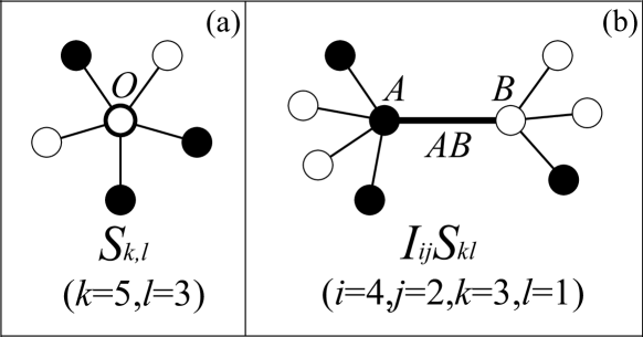
Figure 1: Diagram of the method of node and link classifications. Open symbols ($\circ$) represent susceptible nodes, and solid symbols ($\bullet$) represent infected nodes. (a) The hub node $O$ is a susceptible node. It has five neighbors, in which three are infected. Therefore, this node is in the set $S_{k,l}$ where $k=5$ and $l=3$. (b) The link plotted with the thick straight line, denoted as $AB$, has an infected node, denoted as $A$, at its left end and a susceptible node, denoted as $B$, at its right end. For node $A$, in addition to link $AB$ it has four other links, of which two connect to infected nodes. While for node $B$, in addition to link $AB$ it has three other links, of which one connects to an infected node. Therefore, link $AB$ is in the set $I_{ij}S_{kl}$ with $i=4$, $j=2$, $k=3$, and $l=1$. Besides, node $A$ is in the set $I_{5,2}$ and node $B$ is in the set $S_{4,2}$.

According to the conservation relations that

$$\sum_{i,j,k,l}\left(S_{ij}S_{kl}+I_{ij}I_{kl}+I_{ij}S_{kl}+S_{ij}I_{kl}\right)=1,$$ (3)

and

$$\sum_{k,l}k\left(S_{k,l}+I_{k,l}\right)=\langle k\rangle,$$ (4)

we obtain

$$\sum_{k,l}S_{ij}S_{kl} = (i+1-j)S_{i+1,j}\bigg{/}\sum_{k,l}{k(S_{k,l}+I_{k,l})}$$

$$= (i+1-j)S_{i+1,j}\big{/}\langle k\rangle,$$

$$\sum_{k,l}I_{ij}I_{kl} = (j+1)I_{i+1,j+1}\big{/}\langle k\rangle,$$

$$\sum_{k,l}I_{ij}S_{kl} = (i+1-j)I_{i+1,j}\big{/}\langle k\rangle,$$

$$\sum_{k,l}S_{ij}I_{kl} = (j+1)S_{i+1,j+1}\big{/}\langle k\rangle.$$ (5)

The first equation in Eq. (III) comes from the fact that the summation of $S_{ij}S_{kl}$ with respect to all possible $k$ and $l$ equals the fraction of links connecting an $S_{i+1,j}$ node at one end and an arbitrary S node at the other end.

Further, with the equal footing of two end nodes of a link in an undirected network, we have

$$S_{ij}S_{kl}=S_{kl}S_{ij},\quad I_{ij}I_{kl}=I_{kl}I_{ij},\quad I_{ij}S_{kl}=S_{kl}I_{ij}.$$ (6)

Eqs. (2)-(6) provide the constraints on both node classes and link classes.

Next, we provide initial condition for the sizes of all the classes. Suppose initially a fraction $\varepsilon$ of nodes are randomly selected to be infected. Then, we have

$$S_{k,l} = (1-\varepsilon)p_{k}{k\choose l}\varepsilon^{l}(1-\varepsilon)^{k-l},$$

$$I_{k,l} = \varepsilon p_{k}{k\choose l}\varepsilon^{l}(1-\varepsilon)^{k-l},$$ (7)

and

$$S_{ij}S_{kl} =(1-\varepsilon)^{2}p_{i+1,k+1}{i\choose j}\varepsilon^{j}(1-\varepsilon)^{i-j}{k\choose l}\varepsilon^{l}(1-\varepsilon)^{k-l},$$

$$I_{ij}I_{kl} =\varepsilon^{2}p_{i+1,k+1}{i\choose j}\varepsilon^{j}(1-\varepsilon)^{i-j}{k\choose l}\varepsilon^{l}(1-\varepsilon)^{k-l},$$

$$I_{ij}S_{kl} =\varepsilon(1-\varepsilon)p_{i+1,k+1}{i\choose j}\varepsilon^{j}(1-\varepsilon)^{i-j}{k\choose l}\varepsilon^{l}(1-\varepsilon)^{k-l},$$

$$S_{ij}I_{kl} =(1-\varepsilon)\varepsilon p_{i+1,k+1}{i\choose j}\varepsilon^{j}(1-\varepsilon)^{i-j}{k\choose l}\varepsilon^{l}(1-\varepsilon)^{k-l}.$$

We take $S_{ij}S_{kl}$ as an example to show the reasoning of the above equations. An $S_{ij}S_{kl}$ link has two end nodes with degree $i+1$ and $k+1$, respectively. The probability of picking such a link therefore equals $p_{i+1,k+1}$, and the probability that both of its end nodes being susceptible equals $(1-\varepsilon)^{2}$. Furthermore, the probability that among the $i$ [$k$] links $j$ [$l$] of them connect to infected nodes equals ${i\choose j}\varepsilon^{j}(1-\varepsilon)^{(i-j)}$ [${k\choose l}\varepsilon^{l}(1-\varepsilon)^{(k-l)}$].

After obtaining the constraints and the initial conditions for all the classes, we now provide the corresponding ordinary differential equation (ODE) to describe the time evolution of the system. To simplify the discussion, we separate the whole process into three sub-processes, named “Recovery Process”, “Infection Process” and “Rewiring Process”, respectively. Since during a very short time the mutual influences of these three sub-processes could be ignored, for each class we shall firstly calculate its variations in the three sub-processes, respectively, and then sum them up to obtain the variation of the whole process. Denoting the differential operators of the ODEs describing the three sub-processes and the whole process as “$\textrm{d}^{\textrm{R}}/\textrm{d}t$”, “$\textrm{d}^{\textrm{I}}/\textrm{d}t$”, “$\textrm{d}^{\textrm{W}}/\textrm{d}t$”, and “$\textrm{d}/\textrm{d}t$” respectively, we have $\textrm{d}/\textrm{d}t=\textrm{d}^{\textrm{R}}/\textrm{d}t+\textrm{d}^{\textrm{I}}/\textrm{d}t+\textrm{d}^{\textrm{W}}/\textrm{d}t$.

Firstly, for the Recovery Process, there are two different situations that may cause the variations in the size of the node classes and link classes, respectively. For the node classes $S_{k,l}$ and $I_{k,l}$, the first situation is the change of the infection state that happens on the nodes belonging to $S_{k,l}$ and $I_{k,l}$ (for example, the node $O$ in Fig. 1(a)), and the second one is the change of the infection state that happens on the neighboring nodes of those nodes belonging to $S_{k,l}$ and $I_{k,l}$ (for example, the neighbors of node $O$ in Fig. 1(a)). Similarly, for the link class $X_{ij}Y_{kl}$, where $X$ and $Y$ can be either $S$ or $I$, the first situation is the change of the infection state that happens on the nodes at the ends of the links belonging to $X_{ij}Y_{kl}$ (for example, the nodes $A$ and $B$ in Fig. 1(b)), and the second one is the change of the infection state that happens on the neighboring nodes of those at the ends of the links belonging to $X_{ij}Y_{kl}$ (for example, the nodes other than $A$ and $B$ in Fig. 1(b)). To distinct the two situations, in the formalism describing the Recovery Process provided below, the terms corresponding to the first situation are labelled with “{Self}” on the right side of the equations:

$$\frac{\textrm{d}^{\textrm{R}}S_{k,l}}{\textrm{d}t}= \gamma I_{k,l}$$ {Self}

$$+\gamma[(l+1)S_{k,l+1}-lS_{k,l}],$$ (9)

$$\frac{\textrm{d}^{\textrm{R}}I_{k,l}}{\textrm{d}t}= -\gamma I_{k,l}$$ {Self}

$$+\gamma[(l+1)I_{k,l+1}-lI_{k,l}],$$ (10)

and

$$\frac{\textrm{d}^{\textrm{R}}S_{ij}S_{kl}}{\textrm{d}t}= \gamma I_{ij}S_{kl}+\gamma S_{ij}I_{kl}$$ {Self}

$$-\gamma jS_{ij}S_{kl}+\gamma(j+1)S_{i(j+1)}S_{kl}$$

$$-\gamma lS_{ij}S_{kl}+\gamma(l+1)S_{ij}S_{k(l+1)},$$ (11)

$$\frac{\textrm{d}^{\textrm{R}}I_{ij}I_{kl}}{\textrm{d}t}= -\gamma I_{ij}I_{kl}-\gamma I_{ij}I_{kl}$$ {Self}

$$-\gamma jI_{ij}I_{kl}+\gamma(j+1)I_{i(j+1)}I_{kl}$$

$$-\gamma lI_{ij}I_{kl}+\gamma(l+1)I_{ij}I_{k(l+1)},$$ (12)

$$\frac{\textrm{d}^{\textrm{R}}I_{ij}S_{kl}}{\textrm{d}t}= -\gamma I_{ij}S_{kl}+\gamma I_{ij}I_{kl}$$ {Self}

$$-\gamma jI_{ij}S_{kl}+\gamma(j+1)I_{i(j+1)}S_{kl}$$

$$-\gamma lI_{ij}S_{kl}+\gamma(l+1)I_{ij}S_{k(l+1)},$$ (13)

$$\frac{\textrm{d}^{\textrm{R}}S_{ij}I_{kl}}{\textrm{d}t}= -\gamma S_{ij}I_{kl}+\gamma I_{ij}I_{kl}$$ {Self}

$$-\gamma jS_{ij}I_{kl}+\gamma(j+1)S_{i(j+1)}I_{kl}$$

$$-\gamma lS_{ij}I_{kl}+\gamma(l+1)S_{ij}I_{k(l+1)}.$$ (14)

Diagrams of the Recovery Process described by the above equations are depicted in Figs. 8 (a)-(c).

Similar with the Recovery Process, for the Infection Process there are also two different situations that may cause the variations of the sizes of the node classes $S_{k,l}$ and $I_{k,l}$ and of the link class $X_{ij}Y_{kl}$. The first situation is the change of the infection state that happens on the nodes belonging to $S_{k,l}$ and $I_{k,l}$ or at the ends of $X_{ij}Y_{kl}$, and the second one is the change of the infection state that happens on the neighbors of the nodes referred in the first situation. Now, we give the formalism for the Infection Process. Again, we label “{self}” on the right side of the terms corresponding to the first situation. To facilitate the understanding of the terms describing the second situation, for each term we list the corresponding process it describes in braces on its right side, where “$\sim$” denotes the terms under derivation on the left side of the corresponding equations. Moreover, we provide a detailed explanation of the second term on the right side of Eq. (III) in Appendix A.

$$\frac{\textrm{d}^{\textrm{I}}S_{k,l}}{\textrm{d}t}= -\beta lS_{k,l}$$ {Self}

$$-\beta\sum_{i^{\prime},j^{\prime}}{j^{\prime}S_{i^{\prime}j^{\prime}}S_{(k-1)l}}\langle k\rangle$$

$$+\beta\sum_{i^{\prime},j^{\prime}}{j^{\prime}S_{i^{\prime}j^{\prime}}S_{(k-1)(l-1)}}\langle k\rangle,$$ (15)

$$\frac{\textrm{d}^{\textrm{I}}I_{k,l}}{\textrm{d}t}= \beta lS_{k,l}$$ {Self}

$$-\beta\sum_{i^{\prime},j^{\prime}}{(j^{\prime}+1)S_{i^{\prime}j^{\prime}}I_{(k-1)l}}\langle k\rangle$$

$$+\beta\sum_{i^{\prime},j^{\prime}}{(j^{\prime}+1)S_{i^{\prime}j^{\prime}}S_{(k-1)(l-1)}}\langle k\rangle,$$ (16)

and

$$\frac{\textrm{d}^{\textrm{I}}S_{ij}S_{kl}}{\textrm{d}t}=-\beta jS_{ij}S_{kl}-\beta lS_{ij}S_{kl}$$ {Self}

$$-\beta(i-j)\frac{\sum\limits_{k^{\prime},l^{\prime}}S_{ij}S_{k^{\prime}l^{\prime}}l^{\prime}\langle k\rangle}{(i-j+1)S_{i+1,j}}S_{ij}S_{kl} \{{\scriptscriptstyle{\displaystyle\sim}\rightarrow S_{i(j+1)}S_{kl}}\}$$

$$-\beta(i-j+1)\frac{\sum\limits_{k^{\prime},l^{\prime}}S_{i(j-1)}S_{k^{\prime}l^{\prime}}l^{\prime}\langle k\rangle}{(i-j+2)S_{i+1,j-1}}S_{i(j-1)}S_{kl}$$

$$\{{\scriptscriptstyle S_{i(j-1)}S_{kl}\rightarrow{\displaystyle\sim}}\}$$

$$-\beta(k-l)\frac{\sum\limits_{i^{\prime},j^{\prime}}j^{\prime}S_{i^{\prime}j^{\prime}}S_{kl}\langle k\rangle}{(k-l+1)S_{k+1,l}}S_{ij}S_{kl} \{{\scriptscriptstyle{\displaystyle\sim}\rightarrow S_{ij}S_{k(l+1)}}\}$$

$$-\beta(k-l+1)\frac{\sum\limits_{i^{\prime},j^{\prime}}j^{\prime}S_{i^{\prime}j^{\prime}}S_{k(l-1)}\langle k\rangle}{(k-l+2)S_{k+1,l-1}}S_{ij}S_{k(l-1)},$$

$$\{{\scriptscriptstyle S_{ij}S_{k(l-1)}\rightarrow{\displaystyle\sim}}\}$$ (17)

$$\frac{\textrm{d}^{\textrm{I}}I_{ij}I_{kl}}{\textrm{d}t}=\beta(j+1)S_{ij}I_{kl}+\beta(l+1)I_{ij}S_{kl}$$ {Self}

$$-\beta\frac{\sum\limits_{k^{\prime},l^{\prime}}I_{i(j+1)}S_{k^{\prime}l^{\prime}}(l^{\prime}+1)\langle k\rangle}{I_{i+1,j+1}}I_{ij}I_{kl} \{{\scriptscriptstyle{\displaystyle\sim}\rightarrow I_{i(j+1)}I_{kl}}\}$$

$$+\beta\frac{\sum\limits_{k^{\prime},l^{\prime}}I_{ij}S_{k^{\prime}l^{\prime}}(l^{\prime}+1)\langle k\rangle}{I_{i+1,j}}I_{i(j-1)}I_{kl} \{{\scriptscriptstyle I_{i(j-1)}I_{kl}\rightarrow{\displaystyle\sim}}\}$$

$$-\beta\frac{\sum\limits_{i^{\prime},j^{\prime}}(j^{\prime}+1)S_{i^{\prime}j^{\prime}}I_{k(l+1)}\langle k\rangle}{I_{k+1,l+1}}I_{ij}I_{kl} \{{\scriptscriptstyle{\displaystyle\sim}\rightarrow I_{ij}I_{k(l+1)}}\}$$

$$+\beta\frac{\sum\limits_{i^{\prime},j^{\prime}}(j^{\prime}+1)S_{i^{\prime}j^{\prime}}I_{kl}\langle k\rangle}{I_{k+1,l}}I_{ij}I_{k(l-1)}, \{{\scriptscriptstyle I_{ij}I_{k(l-1)}\rightarrow{\displaystyle\sim}}\}$$

$$\frac{\textrm{d}^{\textrm{I}}I_{ij}S_{kl}}{\textrm{d}t}=\beta jS_{ij}S_{kl}-\beta(l+1)I_{ij}S_{kl}$$ {Self}

$$-\beta(i-j)\frac{\sum\limits_{k^{\prime},l^{\prime}}I_{ij}S_{k^{\prime}l^{\prime}}(l^{\prime}+1)\langle k\rangle}{(i-j+1)I_{i+1,j}}I_{ij}S_{kl} \{{\scriptscriptstyle{\displaystyle\sim}\rightarrow I_{i(j+1)}S_{kl}}\}$$

$$+\beta(i-j+1)\frac{\sum\limits_{k^{\prime},l^{\prime}}I_{i(j-1)}S_{k^{\prime}l^{\prime}}(l^{\prime}+1)\langle k\rangle}{(i-j+2)I_{i+1,j-1}}I_{i(j-1)}S_{kl}$$

$$\{{\scriptscriptstyle I_{i(j-1)}S_{kl}\rightarrow{\displaystyle\sim}}\}$$

$$-\beta\frac{\sum\limits_{i^{\prime},j^{\prime}}j^{\prime}S_{i^{\prime}j^{\prime}}S_{k(l+1)}\langle k\rangle}{S_{k+1,l+1}}I_{ij}S_{kl} \{{\scriptscriptstyle{\displaystyle\sim}\rightarrow I_{ij}S_{k(l+1)}}\}$$

$$+\beta\frac{\sum\limits_{i^{\prime},j^{\prime}}j^{\prime}S_{i^{\prime}j^{\prime}}S_{kl}\langle k\rangle}{S_{k+1,l}}I_{ij}S_{k(l-1)}, \{{\scriptscriptstyle I_{ij}S_{k(l-1)}\rightarrow{\displaystyle\sim}}\}$$

$$\frac{\textrm{d}^{\textrm{I}}S_{ij}I_{kl}}{\textrm{d}t}=-\beta(j+1)S_{ij}I_{kl}+\beta lS_{ij}S_{kl}$$ {Self}

$$-\beta\frac{\sum\limits_{k^{\prime},l^{\prime}}S_{i(j+1)}S_{k^{\prime}l^{\prime}}l^{\prime}\langle k\rangle}{S_{i+1,j+1}}S_{ij}I_{kl} \{{\scriptscriptstyle{\displaystyle\sim}\rightarrow S_{i(j+1)}I_{kl}}\}$$

$$+\beta\frac{\sum\limits_{k^{\prime},l^{\prime}}S_{ij}S_{k^{\prime}l^{\prime}}l^{\prime}\langle k\rangle}{S_{i+1,j}}S_{i(j-1)}I_{kl} \{{\scriptscriptstyle S_{i(j-1)}I_{kl}\rightarrow{\displaystyle\sim}}\}$$

$$-\beta(k-l)\frac{\sum\limits_{i^{\prime},j^{\prime}}(j^{\prime}+1)S_{i^{\prime}j^{\prime}}I_{kl}\langle k\rangle}{(k-l+1)I_{k+1,l}}S_{ij}I_{kl} \{{\scriptscriptstyle{\displaystyle\sim}\rightarrow S_{ij}I_{k(l+1)}}\}$$

$$+\beta(k-l+1)\frac{\sum\limits_{i^{\prime},j^{\prime}}(j^{\prime}+1)S_{i^{\prime}j^{\prime}}I_{k(l-1)}\langle k\rangle}{(k-l+2)I_{k+1,l-1}}S_{ij}I_{k(l-1)}.$$

$$\{{\scriptscriptstyle S_{ij}I_{k(l-1)}\rightarrow{\displaystyle\sim}}\}$$

Diagrams of the Infection process described by the above equations are depicted in Figs. 8 (d)-(f).

Finally, for the Rewiring process, it is composed of two sub-processes. One is the link breaking process, where some susceptible nodes break their links connecting to infected neighbors; and the other is the link attachment process, where susceptible nodes rewire their broken links to other susceptible nodes so as to form new connections. In the following, we give the formalism for the Rewiring Process. We label “{break}” on the right side of all the terms describing the link breaking process; for each term describing the link attachment process we show the corresponding process it describes in braces on its right side with “$\sim$” having the same meaning as that in the Infection Process.

$$\frac{\textrm{d}^{\textrm{W}}S_{k,l}}{\textrm{d}t}= -\omega lS_{k,l}+\omega(l+1)S_{k,l+1}$$ {Break}

$$-\omega(IS)\frac{S_{k,l}}{S}+\omega(IS)\frac{S_{k-1,l}}{S},$$ (21)

$$\frac{\textrm{d}^{\textrm{W}}I_{k,l}}{\textrm{d}t}= -\omega(k-l)I_{k,l}+\omega(k-l+1)I_{k+1,l},$$ {Break}

$$\frac{\textrm{d}^{\textrm{W}}S_{ij}S_{kl}}{\textrm{d}t}= -\omega jS_{ij}S_{kl}+\omega(j+1)S_{i(j+1)}S_{kl}$$ {Break}

$$-\omega lS_{ij}S_{kl}+\omega(l+1)S_{ij}S_{k(l+1)}$$ {Break}

$$-\omega|IS|\frac{S_{ij}S_{kl}\langle k\rangle}{|S|} \{{\scriptscriptstyle{\displaystyle\sim}\rightarrow S_{(i+1)j}I_{kl}}\}$$

$$+\omega|IS|\frac{S_{(i-1)j}S_{kl}\langle k\rangle}{|S|} \{{\scriptscriptstyle S_{(i-1)j}I_{kl}\rightarrow{\displaystyle\sim}}\}$$

$$-\omega|IS|\frac{S_{ij}S_{kl}\langle k\rangle}{|S|} \{{\scriptscriptstyle{\displaystyle\sim}\rightarrow S_{ij}I_{(k+1)l}}\}$$

$$+\omega|IS|\frac{S_{ij}S_{(k-1)l}\langle k\rangle}{|S|} \{{\scriptscriptstyle S_{ij}I_{(k-1)l}\rightarrow{\displaystyle\sim}}\}$$

$$+\omega|IS_{kl}|\frac{S_{i,j}}{|S|}+\omega|S_{ij}I|\frac{S_{k,l}}{|S|},$$

$$\frac{\textrm{d}^{\textrm{W}}I_{ij}I_{kl}}{\textrm{d}t}= -\omega(i-j)I_{ij}I_{kl}$$ {Break}

$$+\omega(i-j+1)I_{(i+1)j}I_{kl}$$ {Break}

$$-\omega(k-l)I_{ij}I_{kl}$$ {Break}

$$+\omega(k-l+1)I_{ij}I_{(k+1)l},$$ {Break}

$$\frac{\textrm{d}^{\textrm{W}}I_{ij}S_{kl}}{\textrm{d}t}= -\omega I_{ij}S_{kl}-\omega(i-j)I_{ij}S_{kl}$$ {Break}

$$+\omega(i-j+1)I_{(i+1)j}S_{kl}$$ {Break}

$$-\omega lI_{ij}S_{kl}+\omega(l+1)I_{ij}S_{k(l+1)}$$ {Break}

$$-\omega|IS|\frac{I_{ij}S_{kl}\langle k\rangle}{|S|} \{{\scriptscriptstyle{\displaystyle\sim}\rightarrow I_{ij}S_{(k+1)l}}\}$$

$$+\omega|IS|\frac{I_{ij}S_{(k-1)l}\langle k\rangle}{|S|}, \{{\scriptscriptstyle I_{ij}S_{(k-1)l}\rightarrow{\displaystyle\sim}}\}$$

$$\frac{\textrm{d}^{\textrm{W}}S_{ij}I_{kl}}{\textrm{d}t}= -\omega S_{ij}I_{kl}-\omega jS_{ij}I_{kl}$$ {Break}

$$+\omega(j+1)S_{i(j+1)}I_{kl}$$ {Break}

$$-\omega(k-l)S_{ij}I_{kl}$$ {Break}

$$+\omega(k-l+1)S_{ij}I_{k(l+1)}$$ {Break}

$$-\omega|IS|\frac{S_{ij}I_{kl}\langle k\rangle}{|S|} \{{\scriptscriptstyle{\displaystyle\sim}\rightarrow S_{(i+1)j}I_{kl}}\}$$

$$+\omega|IS|\frac{S_{(i-1)j}I_{kl}\langle k\rangle}{|S|}, \{{\scriptscriptstyle S_{(i-1)j}I_{kl}\rightarrow{\displaystyle\sim}}\}$$

where $|IS|=\sum_{i,j,k,l}{I_{ij}S_{kl}}$, $|IS_{kl}|=\sum_{i,j}{I_{ij}S_{kl}}$, $|S_{ij}I|=\sum_{i,j}S_{ij}I_{kl}$ and $|S|=\sum_{k,l}S_{k,l}$.

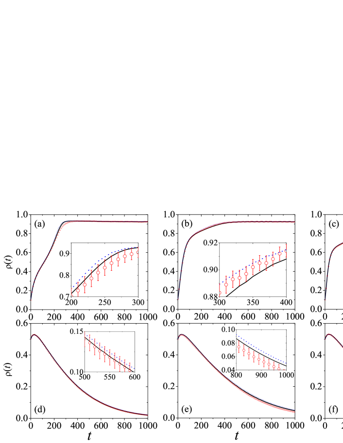
Figure 2: (Color online) Time evolution of the infected fraction $\rho(t)$ for the cases of $\gamma=0.005$, $\omega=0.02$, (a)-(c) $\beta=0.06$, $\varepsilon=0.1$, where the systems eventually evolve to the endemic state, and (d)-(f) $\beta=0.01$, $\varepsilon=0.5$ where the systems eventually evolve to the disease-free state. The black solid curves are obtained from our link-based method; the blue dotted curves are obtained from the node-based method in Ref. Marceau:2010 ; and the red circle symbols are obtained from simulations. Left, middle, and right panels correspond to different cases for $k$-regular network, Poisson network, and power-law network, respectively. The average degrees of all the networks are the same, $\langle k\rangle=2$. For the power-Law network, $k_{T}=13$ and $\tau=2.019$.

The terms describe the link breaking process is relatively easy to understand. For example, the first term on the right side of Eq. (III) means: For the $I_{ij}I_{kl}$ link, the $I_{(i+1),(j+1)}$ node at one of its ends has $(i-j)$ neighboring susceptible nodes. Thus, the probability that the node looses a neighbor in a time step equals $\omega(i-j)$. Once this event happens, an $I_{ij}I_{kl}$ link changes to an $I_{(i-1)j}I_{kl}$ link. Hence, for all the $I_{ij}I_{kl}$ links the probability that one of them changes to the $I_{(i-1)j}I_{kl}$ link in one time step equals $\omega(i-j)I_{ij}I_{kl}$. The link attachment process is a bit more complicated. Specifically, the last term in Eq. (III) denotes the probability of the event that a link previously having the $S_{i+1,j+1}$ node at one end and an infected node at the other end now becomes the $S_{ij}S_{kl}$ links by rewiring itself from the infected node to the $S_{k,l}$ node. To help a better understanding, we give a detailed explanation of the fifth term on the right side of Eq. (III) in the Appendix B. Diagrams of the Rewiring process described by the above equations are depicted in Figs. 8 (g)-(k).

Note that Eqs. (III)-(III) and (III)-(III) do not have any link term $X_{ij}Y_{kl}$, which means in the Recovery Process and Rewiring Process, the link classification information is not directly utilized to calculate the variations of the sizes of the node classes. However, Eqs. (III)-(III) do contain the information of link classes. The information of link classification is utilized to calculate the variations of the sizes of the node classes in the Infection Process. Since the link classification method provides more detailed information of the network structure than the node classification, the accuracy in predicting the time evolution of the node states could be improved by employing our method, as shown in the following section.

IV Simulation results

IV.1 Uncorrelated networks

In the simulations, unless otherwise specified, all the results are obtained based on networks with size $N=10000$ and averaged on $1000$ different realizations.

In this subsection, we will compare our link-based method to the node-based method proposed in Ref. Marceau:2010 . Specifically, we adopt three kinds of initial degree distribution: (i) $k$-regular, where the degrees of all the nodes are the same as $k$. (ii) Poisson distribution, where $p_{k}=z^{k}e^{-z}/k!$ with $z=\langle k\rangle$ being the average degree. This distribution can be achieved from a random-graph model in the limit $N\rightarrow\infty$. (iii) Truncated power-law distribution, where $p_{k}=ck^{-\tau}$ when $0<k<k_{T}$ and $p_{k}=0$ otherwise. For convenience of discussion, we refer to the three kinds of networks as $k$-regular network, Poisson network, and power-law network, respectively.

We start from the case that the initial network topology has no degree correlation. Figure 2 shows the infected fraction $\rho(t)$ for the three kinds of networks, respectively. We observe that both our link-based formalism (solid black curve) and the existing node-based formalism Marceau:2010 (blue dotted curve) have high accuracy in predicting $\rho(t)$. However, detailed plots in the insets of Fig. 2 show that link-based formalism offers better approximation, except for panel (b) where their performances are similar. As mentioned earlier, such improvements are a result of utilizing the link information, which contains more details about the network structure compared with the pure node-based method.

When the proposed formalism is applied on networks with nonempty degree classes, the total number of differential equations is $3(k_{\mathrm{max}}+1)(k_{\mathrm{max}}+2)+3(k_{\mathrm{max}}+1)^{2}(k_{\mathrm{max}}+2)^{2}$ with $k_{\mathrm{max}}$ being the largest degree, which grows with the fourth power of the largest nodal degree. For the node-based method used in Marceau:2010 , the number of the differential equations is $(k_{\mathrm{max}}+1)(k_{\mathrm{max}}+2)$, which is more efficient. Therefore, on uncorrelated networks where the interest is mainly on the infected fraction rather than network topology, the node based method can be a good approximation to describe the system. For the case of correlated networks, however, the following subsection will show that our method can obtain prediction results with high accuracy.

IV.2 Correlated Networks

Now we study how the degree correlation evolves in an adaptive network. We focus on the case where the system in the endemic state could evolve sufficiently and the evolution of the degree correlation is evident. For convenience in presenting the degree correlation, we introduce a relative correlation function defined by $f_{i,k}=p_{i,k}/q_{i}q_{k}$. Obviously, when $f_{i,k}=1$, for all the $i$ and $k$ the network is uncorrelated. For positive (negative) correlated networks, a smaller difference between the values of $i$ and $k$ leads to a larger (smaller) value of $f_{i,k}$.

In our formalisms, the initial joint degree distribution function $p_{i,k}$ can be arbitrary. To verify the formalism, we need to construct networks with a given degree distribution of which the initial degree correlations are tunable so as to satisfy the given $p_{i,k}$. A method to construct networks with arbitrarily given degree correlations is provided in Ref. Weber:2007 , which also proposes an approach for generating a relative correlation function $f_{i,k}$ satisfying a pre-assigned score of factor $r$. Specifically, suppose that the function $f_{i,k}$ is required to satisfy an average nearest-neighbor function $k_{nn}(k)$ with $k_{nn}(k)\propto k^{\alpha}$, where $k_{nn}(k)$ denotes the mean value of the average degree of the nearest neighbors of all the $k$-degree nodes. Then, when $\alpha>0$ the network possesses a positive degree correlation and a larger $\alpha$ corresponds to a larger score of $r$, and vice versa. It is shown that when $f_{i,k}$ is obtained from the following equation, the condition of $k_{nn}(k)\propto k^{\alpha}$ can be satisfied Weber:2007 :

$$f_{i,k}=1+\frac{1}{\langle k^{\alpha}\rangle_{\textrm{e}}}\frac{(i^{\alpha}-\langle k^{\alpha+1}\rangle_{\textrm{e}})(k^{\alpha}-\langle k^{\alpha+1}\rangle_{\textrm{e}})}{\langle k^{\alpha+1}\rangle_{\textrm{e}}/\langle k\rangle_{\textrm{e}}-\langle k^{\alpha}\rangle_{\textrm{e}}},$$ (27)

where $\langle\bullet\rangle_{\textrm{e}}=\sum_{k}{(\bullet\times q_{k})}$. Therefore, by tuning $\alpha$ we may get the desired function $f_{i,k}$ from which a pre-assigned function $k_{nn}(k)$ and correspondingly the desired $r$ score can be obtained.

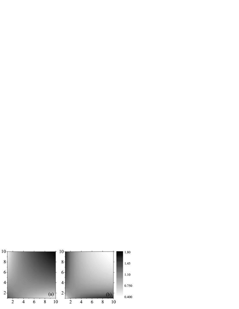
Figure 3: Gray-scale plots of $f_{i,k}$ obtained from Eq. (27), which satisfy the conditions of (a) $r=0.3$ and (b) $r=-0.3$.

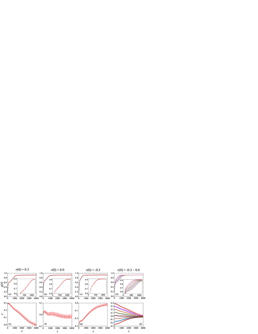
Figure 4: (Color online) The evolution of i) $\rho(t)$ for (a) $r(0)=0.3$, (b) $r(0)=0$, (c) $r(0)=-0.3$; and ii) $r(t)$ for (e) $r(0)=0.3$, (f) $r(0)=0$, (g) $r(0)=-0.3$ respectively, where the initial power-law degree distribution is the same as that in Fig. 2. Panels (d) and (h) show the evolution of $\rho(t)$ and $r(t)$ for different initial $r(0)$. Specifically, in panel (d), curves from above to bottom correspond to the cases of $r(0)=-0.3,\cdots,0.4$, respectively. Symbols represent the simulation results and the curves are obtained from the theoretical formalism. Moreover, the insets of panels (a) - (d) show the zoom in results for the middle stage of the evolution of the corresponding panels. For clarity, the error bars are only shown in the insets of panels (a) - (c), while the sizes of other ones are conform with them. The parameters of the epidemic model are $\gamma=0.0025$, $\beta=0.03$ and $\omega=0.01$.

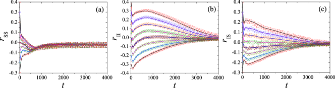
Figure 5: (Color online) The evolution of the correlation measurements of (a) $r_{\textrm{SS}}(t)$, (b) $r_{\textrm{II}}(t)$, and (c) $r_{\textrm{IS}}(t)$ for different initial degree correlations. In all the panels, curves from above to below correspond to the cases of $r(0)=0.4,0.3,0.2,0.1,0,-0.1,-0.2,-0.3$, respectively. Other parameters are the same as those in Fig. 4.

As an example, we show the values of $f_{i,k}$ on the degree-degree plane that are generated by the method introduced above for the cases of $r=0.3$ and $-0.3$ in Figs. 3 (a) and (b), respectively. For the case of $r=0.3$, $f_{i,k}$ with values larger than $1$ are mostly close to the diagonal line especially for the two ends, while for the case of $r=-0.3$, high values of $f_{i,k}$ dominate in the far off-diagonal region.

Since the degree correlation of a degree-regular network is trivial and the degrees of Possion distribution are distributed in a narrow range that largely restricts the range of $r$, we focus our attention on power-law networks. Figures 4 (a)-(d) show the time evolution $\rho(t)$ for different values of $r(0)$ ranging from $-0.3$ to $0.4$, where all the cases are eventually evolve to the endemic state. Detailed plots in Figs. 4 (a)-(c) show that the results obtained from the theoretical formalism (curves) have a good match with the simulation results (symbols). Moreover, as shown in Fig. 4 (d), in the middle stage of evolution, cases with smaller $r(0)$ always have higher $\rho(t)$ than those with larger $r(0)$, meaning that negative initial correlation favors the spreading of infection in this case. Figures 4 (e)-(h) show the evolution of $r(t)$ for the corresponding cases in (a)-(d), respectively. Figure 4 (h) shows that $r(t)$ moves gradually towards zero in all the cases, which indicates that the memory of the initial degree correlation fades out since the nodal degree is not discriminated during the Rewiring Process. Finally, for all the cases, $\rho(t)$ converge to the same value.

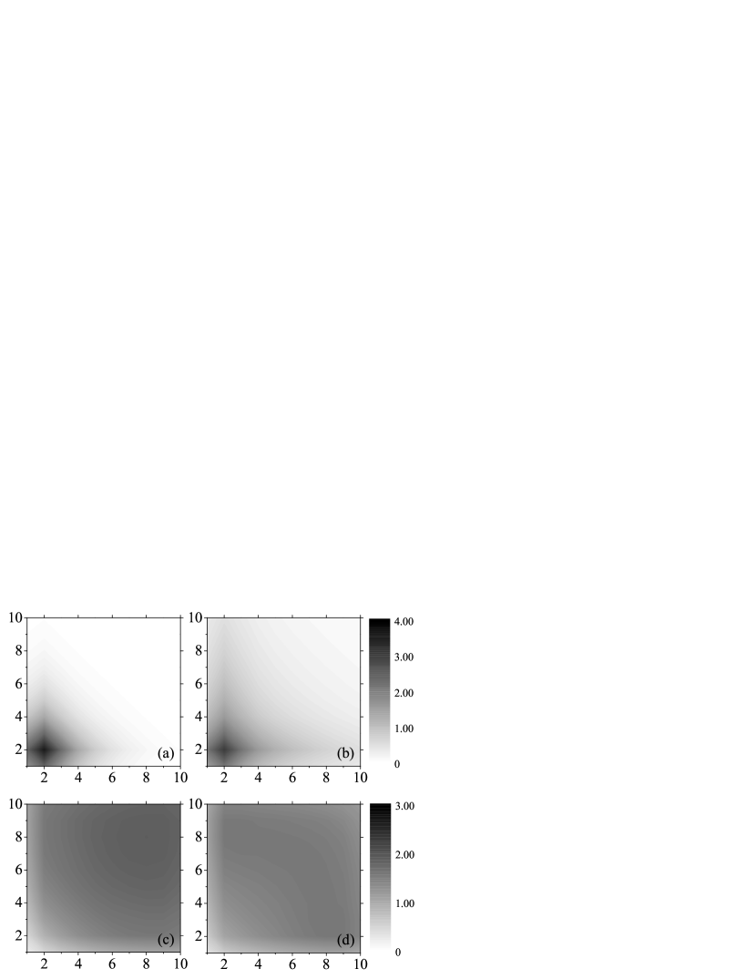
Figure 6: Gray-scale plots the ratio $p_{i,k}^{\textrm{SS}}(t=60)/p_{i,k}^{\textrm{SS}}(t=0)$ for the cases of (a) $r(0)=0.3$ and (b) $r(0)=-0.3$, and the ratio $p_{i,k}^{\textrm{II}}(t=60)/p_{i,k}^{\textrm{II}}(t=0)$ for the cases of (c) $r(0)=0.3$ and (d) $r(0)=-0.3$ on the degree-degree plane. Other parameters are the same as those in Fig. 4.

To study the degree correlation more carefully, we further introduce several measures according to the nodes states at the ends of edges. Specifically, we use $r_{\textrm{SS}}$, $r_{\textrm{II}}$, $r_{\textrm{IS}}$ to measure the degree correlations for the links whose ends are attached by two S nodes, two I nodes, and one S node and one I node, respectively. By using the Pearson correlation, these measures are defined as

$$r_{\textrm{XY}}=\frac{1}{\sigma_{e}^{\textrm{X}}\sigma_{e}^{\textrm{Y}}}\sum_{i,k}(p_{i,k}^{\textrm{XY}}-q_{i}^{\textrm{X}}q_{k}^{\textrm{Y}}),$$ (28)

where X and Y can be either S or I. In the definition, $p_{i,k}^{\textrm{SS}}$ denotes the probability that an SS link are attached by an $i$-degree S node and a $k$-degree S node, and $q_{i}^{\textrm{S}}$ is defined as $q_{i}^{\textrm{S}}=\sum_{k}{p_{i,k}^{\textrm{SS}}}$ denoting the edge end distribution of all the S nodes reached by the SS links. Hence, we have $\sum_{i,k}{p_{i,k}^{\textrm{SS}}=1}$, and $\sum_{i}{q_{i}^{\textrm{S}}}=1$, and $\sigma_{e}^{\textrm{S}}=\left({\sum_{i}{i^{2}q_{i}^{\textrm{S}}}-(\sum_{i}{iq_{i}^{\textrm{S}}})^{2}}\right)^{1/2}$. Moreover, $p_{i,k}^{\textrm{II}}$, $p_{i,k}^{\textrm{IS}}$, $q_{i}^{\textrm{I}}$ and $\sigma_{e}^{\textrm{I}}$ are similarly defined. For the initial condition, suppose that a fraction $\varepsilon$ of nodes are randomly selected as infected nodes. Then, the number of SS links whose ends are attached by an $i$-degree S node and a $k$-degree S node can be calculated as $(1-\varepsilon)(1-\varepsilon)p_{i,k}M$, and the total number of SS links is $(1-\varepsilon)(1-\varepsilon)\sum_{i,k}{p_{i,k}}M=(1-\varepsilon)(1-\varepsilon)M$ with $M$ being the total number of the connections. Therefore, we have $p_{i,k}^{\textrm{SS}}/\sum_{i,k}p_{i,k}^{\textrm{SS}}=p_{i,k}/\sum_{i,k}p_{i,k}$ and consequently $r_{\textrm{SS}}(0)=r(0)$. With similar analysis, we obtain $r(0)=r_{\textrm{SS}}(0)=r_{\textrm{II}}(0)=r_{\textrm{IS}}(0)$.

Figure 5 shows the evolution of these measures for the cases studied in Fig. 4. We can observe that, in all cases, $r_{\textrm{SS}}$ goes to $0$ most quickly as compared with other measures and $r_{\textrm{II}}$ have a significant drop in the beginning stage of the evolution. Besides, the speed of $r_{\textrm{IS}}$ moving towards $0$ is between those of $r_{\textrm{SS}}$ and $r_{\textrm{II}}$. This phenomenon can be understood as follows: for the susceptible nodes, those have larger degree can be infected more easily as they have more infected neighbors on average. Thus, the number of large-degree S nodes reduces quickly, which makes the degrees of the nodes at the ends of SS links quickly tend to small value. As a small-degree range confines the degree correlation at a low level, the value of $r_{\textrm{SS}}$ reduces accordingly. On the other hand, since in the beginning stage, large-degree susceptible nodes are easily infected, which contributes to the increase of the number of large-degree infected nodes and these large-degree infected nodes probably have infected neighbors with smaller degree, they could form II links with a negative correlation.

To verify our explanation, we plot the ratios of $p_{i,k}^{\textrm{SS}}$ and $p_{i,k}^{\textrm{II}}$ at $t=60$ to that at $t=0$ for the case of $r(0)=0.3$ in Fig. 6 (a) and (c) and for the case of $r(0)=-0.3$ in Fig. 6 (b) and (d), respectively. We observe that for both cases SS links mainly converge to the point (2,2) on the degree plane with $2$ being the average degree in this case at $t=60$, while $p_{i,k}^{\textrm{II}}$ increases in the large-degree range. In other words, for the case of $r(0)=-0.3$, the ratio of $p_{i,k}^{\textrm{II}}$ has an obvious increase in the negative correlation region.

V Conclusion

We have introduced a link-based formalism to present the adaptive network model proposed by Gross et al. Gross:2006 . In our method, inspired by the node classification method Marceau:2010 and master equations approach Gleeson:2011 , we took link as the object and classify them according to the disease states, the number of neighbors, and the number of infected neighbors of each node at its ends. Moreover, for clarity, we have separated the whole dynamics into three sub-processes, namely Recovery Process, Infection Process and Rewiring Process. For each process, a set of differential equations is established to describe the evolution of each class of links. By combining all these equations together, an integrated formalism describing the time evolution of the adaptive networks is established.

Our formalism provides subtle detailed information of degree correlation. It can predict the evolution of the system with higher accuracy than former node-based method where the network was treated under zero degree correlation approximation. More importantly, it can offer a more precise description of the network structure. Since the network topology is one of the key ingredients of an adaptive network, in-depth observation of the topology is of importance to reveal how the network topology and the nodal dynamics coevolve. Thus, our theoretical formalism could be a valuable improvement in understanding the mechanism of adaptive networks.

To reveal further details than those by the degree correlation measure $r$ Newman:2002 , we have introduced other degree correlation measures $r_{\textrm{SS}}$, $r_{\textrm{II}}$, $r_{\textrm{IS}}$ according to the disease states of the nodes at the ends of the links. We found that although the time evolution of $r$ is relatively steady, the evolutions of $r_{\textrm{SS}}$, $r_{\textrm{II}}$ are not. Specifically, $r_{\textrm{SS}}$ moves to zero most quickly among all the measurements, while $r_{\textrm{II}}$ has a significant drop in the beginning stage. An explanation of this phenomenon can be provided with our formalism.

In this work, we assume that when susceptible nodes are rewiring their broken links, they do not consider the nodal degree of the susceptible nodes to be selected. Thus, the system will tend to zero (or a near zero) correlation when the evolving time is long enough. However, in a more general situation, nodes may consider the nodal degrees of each other, and hence the system could possess non-zero correlation all the time. For this more general situation, our link-based method might be extended to handle the degree correlation in predicting the dynamics of such systems, and this will be a future research topic.

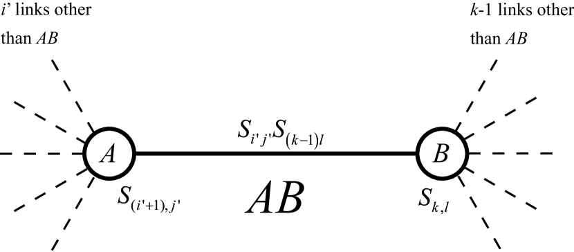
Figure 7: Diagram of an $S_{k,l}$ node, denoted as $B$, connected with an $S_{(i^{\prime}+1),j^{\prime}}$ node, denoted as $A$, through an $S_{i^{\prime}j^{\prime}}S_{(k-1)l}$ link, denoted as $AB$.

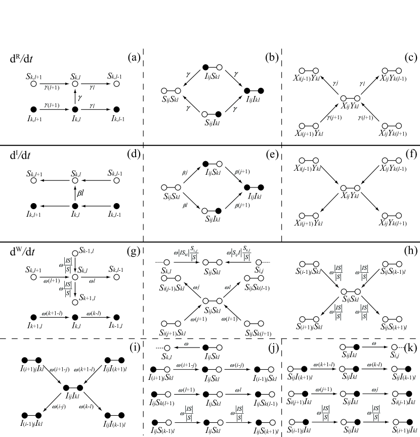
Figure 8: Diagram of the variations of node/link class sizes in the Recovery Process $\textrm{d}^{\textrm{R}}/\textrm{d}t$ (a) - (c), the Infection Process $\textrm{d}^{\textrm{I}}/\textrm{d}t$ (d) - (f), and the Rewiring Process $\textrm{d}^{\textrm{W}}/\textrm{d}t$ (g) - (k). Open symbols ($\circ$) represent the susceptible nodes and solid symbols ($\bullet$) represent the infected nodes. $A\rightarrow B$ means the state of node or link represented by $A$ changes to that represented by $B$, and the term near an arrow ’$\rightarrow$’ indicates the rate of the corresponding change. Specifically, panel (a) [(d)] indicates the variations of the node states in the Recovery [Infection] Process, panel (b) [(e)] indicates the variations of the link states caused by the state change of the nodes at their ends, and panel (c) [(f)] indicates the variations of the links states caused by the state change of the neighbors of the their end nodes. In panels (c) and (f), $X$ and $Y$ can be either $S$ or $I$. In panel (f) the rates are complicated therefore are not shown here; details can be found in the text. Panel (g) indicates the variations of the node states in the Rewiring Process. Panel (h), (i), (j), (k) indicate the variation of the link states for the SS link, II link, IS link and SI link in the Rewiring Process, respectively, where $|IS|=\sum_{i,j,k,l}I_{ij}S_{kl}$, $|IS_{kl}|=\sum_{i,j}I_{ij}S_{kl}$, $|S_{ij}I|=\sum_{k,l}S_{ij}I_{kl}$, and $|S|=\sum_{k,l}S_{k,l}$.

Chapter

Appendix A Derivation of the second term on the right hand side of Eq. (III)

This term is $-\beta\sum_{i^{\prime},j^{\prime}}{j^{\prime}S_{i^{\prime}j^{\prime}}S_{(k-1)l}\langle k\rangle}$, which denotes the rate of the process that $S_{k,l}$ nodes change to $S_{k,l+1}$. This process happens when one of the susceptible neighbors of an $S_{k,l}$ node is infected.

As shown in Fig. 7, we use $B$ to denote an $S_{k,l}$ node. Suppose that node $B$ has a neighbor $A$ which is an $S_{(i^{\prime}+1),j^{\prime}}$ node. Then, the link, denoted as $AB$, connecting $A$ and $B$, is an $S_{i^{\prime}j^{\prime}}S_{(k-1)l}$ link. Here, $k-1$ comes when we count the number of the neighbors of node $B$ we exclude the present link $AB$. Moreover, since node $A$ is in S state, we could infer that among the other $k-1$ neighbors of node $B$, $l$ of them are infected. Therefore, the fourth subscript of the link class that $AB$ belongs to is $l$. The meaning of $i^{\prime}$ and $j^{\prime}$ could be understood similarly. Since node $A$ has $j^{\prime}$ infected neighbors, the probability that it is infected in one time step equals $\beta j^{\prime}$.

Now, the question is: what is the probability that the node $A$ is an $S_{(i^{\prime}+1),j^{\prime}}$ node? This is equivalent to ask: what is the probability that a link connecting node $B$ is an $S_{i^{\prime}j^{\prime}}S_{(k-1)l}$ link. Here, we use the mean-field theory to estimate it. The total number of the links that have an $S_{k,l}$ node on one end and another S state node on the other end equals $(k-l)S_{k,l}N$. Among them, $S_{i^{\prime}j^{\prime}}S_{(k-1)l}\langle k\rangle N$ links satisfy the condition that one end is an $S_{k,l}$ node and the other end is an $S_{(i^{\prime}+1),j^{\prime}}$ node. Therefore, on average the probability that a link connecting node $B$ is an $S_{i^{\prime}j^{\prime}}S_{(k-1)l}$ link equals $[S_{i^{\prime}j^{\prime}}S_{(k-1)l}\langle k\rangle N]/[(k-1)S_{k,l}N]$, and this probability is also the one that node $A$ is an $S_{(i^{\prime}+1),j^{\prime}}$ node.

Since an $S_{(i^{\prime}+1),j^{\prime}}$ node has $j^{\prime}$ infected neighbors, the probability that node $A$ is an $S_{(i^{\prime}+1),j^{\prime}}$ node and gets infection in one time step equals $[\beta j^{\prime}S_{i^{\prime}j^{\prime}}S_{(k-1)l}\langle k\rangle]/[(k-l)S_{k,l}]$.

Furthermore, by summing up all the possible node classes that node $A$ may belong to, we obtain the probability that a susceptible neighbor of $B$ gets infection in one time step, as $[\beta\sum_{i^{\prime},j^{\prime}}j^{\prime}S_{i^{\prime}j^{\prime}}S_{(k-1)l}\langle k\rangle]/[(k-l)S_{k,l}]$.

Since node $B$ has $(k-l)$ links connecting to its S state neighbors, the rate that $S_{k,l}$ nodes change to $S_{k,l+1}$ equals $(k-l)S_{k,l}[\beta\sum_{i^{\prime},j^{\prime}}j^{\prime}S_{i^{\prime}j^{\prime}}S_{(k-1)l}\langle k\rangle]/[(k-l)S_{k,l}]$. Finally, since this process leads to the decrease of the fraction of $S_{k,l}$ nodes, we come to the result $-\beta\sum_{i^{\prime},j^{\prime}}{j^{\prime}S_{i^{\prime}j^{\prime}}S_{(k-1)l}\langle k\rangle}$.

Chapter

Appendix B Derivation of the fifth term on the right hand side of Eq. (III)

This term is $-\omega|IS|S_{ij}S_{kl}\langle k\rangle/|S|$, which denotes the rate of the process that links $S_{ij}S_{kl}$ change to $S_{(i+1)j}S_{kl}$. This process happens when an $S_{(i+1),j}$ node at one end of an $S_{ij}S_{kl}$ link is chosen in rewiring to form a new link.

First, the total amount of broken links is $\omega|IS|$ with $|IS|=\sum_{i,j,k,l}{I_{ij}S_{kl}}$ being the total amount of IS link. Then, for each broken link, the probability that it chooses an $S_{(i+1),j}$ node equals $S_{(i+1),j}/|S|$, where $|S|=\sum_{k,l}S_{k,l}$. When an $S_{(i+1),j}$ node is chosen by a rewired link, the states of the links attached on this node will also be changed. By adopting the mean-filed theory approximation, for a link attached on an $S_{(i+1),j}$ node, the probability that it is an $S_{ij}S_{kl}$ link equals $[S_{ij}S_{kl}\langle k\rangle N]/[(i-j+1)S_{i+1,j}N]$, where the denominator represents the total number of the links of which one end is an $S_{(i+1),j}$ node and the other end is a susceptible node, while the numerator represents the number of $S_{ij}S_{kl}$ links. Since an $S_{(i+1),j}$ node has $(i-j+1)$ such links, the average number of the $S_{ij}S_{kl}$ links that an $S_{(i+1),j}$ node has is equal to $\{(S_{ij}S_{kl}\langle k\rangle N)/[(i-j+1)S_{i+1,j}N]\}(i-j+1)$.

Summing up all the above, the portion that the $S_{ij}S_{kl}$ links changing to $S_{(i+1)j}S_{kl}$ links in this process equals $\omega|IS|\{S_{i+1,j}/|S|\}\{S_{ij}S_{kl}\langle k\rangle N/[(i-j+1)S_{i+1,j}N]\}(i-j+1)$. Since this process leads to the decrease of the fraction of $S_{ij}S_{kl}$ links, we come to the conclusion that the item is $-\omega|IS|(S_{ij}S_{kl}\langle k\rangle)/|S|$.

Chapter

Appendix C A comprehensive diagram of all the processes described in the ODEs

This diagram is shown in Fig. 8.

- (1) Duncan J. Watts, Pro. Nat. Acad. Sci. 99, 5766 (2002).
- (2) C. Nardini, B. Kozma, and A. Barrat, Phys. Rev. Lett. 100, 158701 (2008).
- (3) P. Holme, and M. E. J. Newman, Phys. Rev. E 74, 056108 (2006).
- (4) F. Vazquez, V. M. Egu luz, and M. S. Miguel, Phys. Rev. Lett. 100, 108702 (2008).
- (5) R. Pastor-Satorras, and A. Vespignani, Phys. Rev. Lett. 86, 3200 (2001).
- (6) M. Barthélemy, A. Barrat, R. Pastor-Satorras, and A. Vespignani, Phys. Rev. Lett. 92, 178701 (2004).
- (7) P.-A. Noël, B. Davoudi, R. C. Brunham, L. J. Dubé, and B. Pourbohloul, Phys. Rev. E 79, 026101 (2009).
- (8) J. Zhou, N. N. Chung, L. Y. Chew, and C.-H. Lai, Phys. Rev. E 86, 026115 (2012).
- (9) Z. H. Liu, and B. Hu, Europhys. Lett. 72, 315 (2005).
- (10) M. Tang, Z. H. Liu, and B. W. Li, Europhys. Lett. 87, 18005 (2009).
- (11) J. Zhou, Z. H. Liu, and B. W. Li, Phys. Lett. A 368, 458 (2007).
- (12) S. N. Dorogovtsev, A. V. Goltsev and J. F. F. Mendes, Phys. Rev. E 66, 016104 (2002).
- (13) A. V. Goltsev, F. V. de Abreu, S. N. Dorogovtsev, and J. F. F. Mendes, Phys. Rev. E 81, 061921 (2010).
- (14) J. A. Acebrón, S. Lozano, and A. Arenas, Phys. Rev. Lett. 99, 128701 (2007).
- (15) J. Zhou, Y. Z. Zhou, and Z. H. Liu, Phys. Rev. E 83, 046107 (2011).
- (16) T. Gross, Carlos J. Dommar D’Lima, and B. Blasius, Phys. Rev. Lett. 96, 208701 (2006).
- (17) J. Zhou, G. Xiao, S. A. Cheong, X. Fu, L. Wong, S. Ma, and T. H. Cheng, Phys. Rev. E 85, 036107 (2012).
- (18) T. Gross, and I. G. Kevrekidis, Europhysics Lett 82, 38004 (2008).
- (19) V. Marceau, P.-A. Noël, L. Hébert-Dufresne, A. Allard, and L. J. Dubé, Phys. Rev. E 82, 036116 (2010).
- (20) J. P. Gleeson, Phys. Rev. Lett. 107, 068701 (2011).
- (21) G. Demirel, F. Vazquez, G.A. B hme, T. Gross, arXiv:1211.0449 (2012).
- (22) Richard Durrett, James P. Gleeson, Alun L. Lloyd, Peter J. Mucha, Feng Shi, David Sivakoff, Joshua E. S. Socolar, and Chris Varghese, Proc. Natl. Acad. Sci. U.S.A. 109, 3682 (2012).
- (23) J. P. Gleeson, Phys. Rev. X 3, 021004 (2013).
- (24) M. E. J. Newman, Phys. Rev. Lett. 89, 208701 (2002).
- (25) As to the notations of the classes, for node classes the pair of subscripts are separated with a comma (e.g. ); for link classes the two pairs of subscripts are not separated, as a distinction to node classes (e.g. ). When a subscript of a link class has “” or “”, we put it between a pair of parentheses for indication (e.g. ). However, parentheses are not used for node classes when a subscript has “” or “” (e.g. ).
- (26) S. Weber, and M. Porto, Phys. Rev. E 76, 046111 (2007).