On radial stationary solutions to a model of nonequilibrium growth

Abstract

We present the formal geometric derivation of a nonequilibrium growth model that takes the form of a parabolic partial differential equation. Subsequently, we study its stationary radial solutions by means of variational techniques. Our results depend on the size of a parameter that plays the role of the strength of forcing. For small forcing we prove the existence and multiplicity of solutions to the elliptic problem. We discuss our results in the context of nonequilibrium statistical mechanics.

1 Introduction

Epitaxial growth is characterized by the deposition of new material on existing layers of the same material under high vacuum conditions. This technique is used in the semiconductor industry for the growth of thin films [5]. The crystals grown may be composed of a pure chemical element like silicon or germanium, or may either be an alloy like gallium arsenide or indium phosphide. In case of molecular beam epitaxy the deposition takes place at a very slow rate and almost atom by atom. The goal in most situations of thin film growth is growing an ordered crystal structure with flat surface. But in epitaxial growth it is quite usual finding a mounded structure generated along the surface evolution [19]. The actual origin of this mounded structure is to a large extent unknown, although some mechanisms (like energy barriers) have already been proposed. Attempting to perform ab initio quantum mechanical calculations in this system is computationally too demanding, what opens the way to the introduction of simplified models. These have been usually developed within the realm of non-equilibrium statistical mechanics, and can be of a discrete probabilistic nature or have the form of a differential equation [5]. Discrete models usually represent adatoms (the atoms deposited on the surfaces) as occupying lattice sites. They are placed randomly at one such site and then they are allowed to move according to some rules which characterize the different models. A different modelling possibility is using partial differential equations, which in this field are frequently provided with stochastic forcing terms. In this work we will focus on rigorous and numerical analyses of ordinary differential equations related to models which have been introduced in the context of epitaxial growth. We hope that a systematic mathematical study will contribute to the understanding of this sort of processes, which are relevant both in pure physics and its industrial applications, in the long term.

The mathematical description of epitaxial growth uses the function

$$u:\Omega\subset\mathbb{R}^{2}\times\mathbb{R}^{+}\rightarrow\mathbb{R},$$ (1.1)

which describes the height of the growing interface in the spatial point $x\in\Omega\subset\mathbb{R}^{2}$ at time $t\in\mathbb{R}^{+}$. Although this theoretical framework can be extended to any spatial dimension $N$, we will concentrate here on the physical situation $N=2$. A basic modelling assumption is of course that $u$ is an univalued function, a fact that holds in a reasonably large number of cases [5]. The macroscopic description of the growing interface is given by a partial differential equation for $u$ which is usually postulated using phenomenological and symmetry arguments [5, 20]. A prominent example of such a theory is given by the Kardar-Parisi-Zhang equation [17]

$$u_{t}=\nu\Delta u+\gamma|\nabla u|^{2}+\eta(x,t),$$ (1.2)

which has been extensively studied in the physical literature and it is currently being investigated for its interesting mathematical properties [1, 2]. It has been argued however that epitaxial growth processes should be described by some equation coming from a conservation law and, in particular, that the term $|\nabla u|^{2}$ should not be present in such an equation [5]. To this end, among others, the conservative counterpart of the Kardar-Parisi-Zhang equation was introduced [21, 22, 18]

$$u_{t}=-\mu\Delta^{2}u+\kappa\Delta|\nabla u|^{2}+\zeta(x,t).$$ (1.3)

This equation is conservative in the sense that the first moment $\int_{\Omega}u\,dx$ is constant if the appropriate boundary conditions are used. It can be considered as a higher order counterpart of the Kardar-Parisi-Zhang equation, and it poses as well a number of fundamental mathematical questions [7, 8, 9].

In this work we will focus on a variation of the last equation. Its formal derivation will be presented in the following section. The remainder of this work will be devoted to clarify the analytical properties of the radial stationary solutions to the model under consideration.

2 Formal derivation of the model

Herein we will adopt a variational formulation of the surface growth equation, which has been postulated as a simple and yet physically relevant way of developing growth models [20]. In order to proceed with our formal derivation, we will assume that the height function obeys a gradient flow equation with a forcing term

$$u_{t}=\sqrt{1+(\nabla u)^{2}}\left[-\frac{\delta\mathcal{J}(u)}{\delta u}+\xi(x,t)\right].$$ (2.1)

The functional $\mathcal{J}$ denotes a potential which describes the microscopic properties of the interface and, at the macroscopic scale, it is assumed that it can be expressed as a function of the surface mean curvature only [20]

$$\mathcal{J}(u)=\int_{\Omega}F(H)\,\sqrt{1+(\nabla u)^{2}}\,\,dx,$$ (2.2)

where the presence of the square root terms models growth along the normal to the surface, $H$ denotes the mean curvature and $F$ is an unknown function of $H$. We will furthermore assume that this function can be expanded in a power series

$$F(H)=K_{0}+K_{1}H+\frac{K_{2}}{2}H^{2}+\frac{K_{3}}{6}H^{3}+\cdots,$$ (2.3)

and subsequently formally apply the small gradient expansion, which assumes $|\nabla u|\ll 1$. This is a classical approximation in this physical context [20] and it is basic in the derivation of the Kardar-Parisi-Zhang equation [17] among others. In the resulting equation, only linear and quadratic terms in the field $u$ and its derivatives are retained, as higher order nonlinearities are assumed not to be relevant in the large scale description of a growing interface [5]. The final result reads

$$u_{t}=K_{0}\,\Delta u+2\,K_{1}\,\det\left(D^{2}u\right)-K_{2}\,\Delta^{2}u-\frac{1}{2}\,K_{3}\,\Delta\left(\Delta u\right)^{2}+\xi(x,t),$$ (2.4)

which is, as well as (1.3), a conservative equation in the sense that $\int_{\Omega}u\,dx$ is constant if appropriate boundary conditions are used. We note that powers of the mean curvature higher than the cubic one in expansion (2.3) do not contribute to equation (2.4) as they imply cubic or higher nonlinearities of the field $u$ or its derivatives. The terms in equation (2.4) have a clear geometrical meaning. The term proportional to $K_{0}$ is the result of the minimization of the zeroth order of the mean curvature, that is, it corresponds to the minimization of the surface area. Its functional form simply reduces to standard diffusion. The term proportional to $K_{1}$ comes from the minimization of the mean curvature and actually it is the determinant of the Hessian matrix, which is nothing but the small gradient approximation of the surface Gaussian curvature. So we see that, through the small gradient approximation, a gradient flow pursuing the minimization of the mean curvature leads to a evolution which favors the growth of the Gaussian curvature. The term proportional to $K_{2}$ comes from the minimization of the squared mean curvature. A functional involving the squared mean curvature is known as Willmore functional and it has its own status within differential geometry [23]. The bilaplacian accompanying $K_{2}$ is the corresponding linearized Euler-Lagrange equation of the Willmore functional when looking for flat minimizers, and it has already appeared in the context of mathematical elasticity [16]. Finally the term proportional to $K_{3}$ comes from the minimization of the cubic power of the mean curvature and it involves a nonlinear combination of Laplacians of the field. We note that from a more puristic geometrical viewpoint one would retain only even powers of the mean curvature in expansion (2.3), which would give rise to a symmetric solution to the corresponding simplification of equation (2.4) (i. e., a solution invariant to the transformation $u\to-u$). However, from a physical viewpoint, we are seeking for a solution to a partial differential equation which represents the interface between two different media (solid structure and vacuum in the present case) so this symmetry is not guaranteed a priori, and we need to retain the odd powers of the mean curvature in expansion (2.3).

For our current purposes we will focus on the associated stationary problem to a simplification of equation (2.4). Such an equation can be obtained employing well known facts from the theory of non-equilibrium surface growth. We may invoke classical scaling arguments in the physical literature to disregard the last term as a higher order correction which will not be present in the description of the largest scale properties of the evolving surface [5]. This practically reduces to setting $K_{3}=0$ in equation (2.4). In epitaxial growth one may phenomenologically set $K_{0}=0$, and we will assume so for the rest of this work. The underlying physical reason is that the diffusion proportional to $K_{0}$ is triggered by the effect of gravity on adatoms, and this effect is negligible in the case of epitaxial growth [5]. The resulting equation reads

$$u_{t}=2\,K_{1}\,\det\left(D^{2}u\right)-K_{2}\,\Delta^{2}u+\xi(x,t).$$ (2.5)

This partial differential equation can be thought of as been an analogue of equation (1.3). Indeed, it has been shown that this equation might constitute a suitable description of epitaxial growth in the same sense equation (1.3) is so, and it even shows more intuitive geometric properties [11]. So, at the physical level, we can consider equation (2.5) as a higher order conservative counterpart of the Kardar-Parisi-Zhang equation. At the mathematical level we can consider it as a sort of Gaussian curvature flow [6, 4] which is stabilized by means of a higher order viscosity term. Furthermore, this viscosity term, as we have seen, has a clear geometrical meaning. As we explain above, in this work we are concerned with the stationary version of (2.5), which reads

$$\left\{\begin{array}[]{rcl}\Delta^{2}u&=&\text{det}\left(D^{2}u\right)+\lambda f,\qquad x\in\Omega\subset\mathbb{R}^{2},\\ \text{boundary}&&\text{ conditions,}\end{array}\right.$$ (2.6)

after getting rid of the equation constant parameters by means of a trivial re-scaling of field and coordinates. Our last assumption is that the forcing term $f=f(x)$ is time independent. This type of forcing is known in the physical literature as columnar disorder, and it has an actual experimental meaning within the context of non-equilibrium statistical mechanics [14]. The constant $\lambda$ is a measure of the intensity of the rate at which new particles are deposited, and for physical reasons we assume $\lambda\geq 0$ and $f(x)\geq 0$. We will devote our efforts to rigorously and numerically clarify the existence and multiplicity of solutions to this elliptic problem when set on a radially symmetric domain.

3 Radial problems

3.1 Dirichlet boundary conditions

We start looking for radially symmetric solutions of boundary value problem (2.6) with $f=f(r)$, where $r$ is the radial coordinate, and homogeneous Dirichlet boundary conditions. We set the problem on the unit disk. That is, we look for solutions of the form $u=\tilde{u}(r)$ where

$$r=\sqrt{x_{1}^{2}+x_{2}^{2}}.$$

By means of a direct substitution we find

$$\frac{1}{r}\left\{r\left[\frac{1}{r}\left(r\tilde{u}^{\prime}\right)^{\prime}\right]^{\prime}\right\}^{\prime}=\frac{1}{r}\,\tilde{u}^{\prime}\tilde{u}^{\prime\prime}+\lambda f(r),$$ (3.1)

where ${}^{\prime}=\frac{d}{dr}$, and the conditions $\tilde{u}^{\prime}(0)=0$, $\tilde{u}(1)=0$, $\tilde{u}^{\prime}(1)=0$, and $\lim_{r\to 0}ru^{\prime\prime\prime}(r)=0$; the first one imposes the existence of an extremum at the origin and the second and third ones are the actual boundary conditions. The fourth boundary condition is technical and imposes higher regularity at the origin. If this condition were removed this would open the possibility of constructing functions $u(r)$ whose second derivative had a peak at the origin. This would in turn imply the presence of a measure at the origin when calculating the fourth derivative of such an $u(r)$, so this type of function cannot be considered as an acceptable solution of (3.1) whenever $f(r)$ is a function. Throughout this section we will assume $f\in L^{1}([0,1],r\,dr)$, that is $f$ is an absolutely integrable function against measure $r\,dr$ on the unit interval, and we drop the tilde on $\tilde{u}$ in order to simplify the notation.

Now we proceed to prove the existence of at least two solutions to this boundary value problem. From now on we will employ the functional space $\mathring{W}^{2,2}([0,1],r\,dr)$, which is the closure of the space of radially symmetric smooth functions compactly supported inside the unit ball of $\mathbb{R}^{2}$ with the norm of $W^{2,2}([0,1],r\,dr)$. We will look for solutions to our problem within this functional space.

Lemma 3.1.

Differential equation (3.1) subjected to Dirichlet boundary conditions is the Euler-Lagrange equation of functional

$$\left\{\begin{array}[]{rcl}J_{\lambda}:&\mathring{W}^{2,2}([0,1],r\,dr)&\rightarrow\mathbb{R}\\ &u&\rightarrow J_{\lambda}\left(u\right)=\frac{1}{2}\int_{0}^{1}\left[\left(u^{\prime\prime}\right)^{2}+\frac{\left(u^{\prime}\right)^{2}}{r^{2}}\right]r\,dr\\ &&\hskip 56.9055pt+\frac{1}{6}\int_{0}^{1}\left(u^{\prime}\right)^{3}dr-\lambda\int_{0}^{1}f\,u\,r\,dr.\end{array}\right.$$ (3.2)

Proof.

We consider Euler first variation of functional (3.2)

$$\left.\frac{d}{dt}J_{\lambda}(u+t\phi)\right|_{t=0} =$$

$$= \int_{0}^{1}\left[u^{\prime\prime}\phi^{\prime\prime}+\frac{u^{\prime}\phi^{\prime}}{r^{2}}\right]r\,dr+\frac{1}{2}\int_{0}^{1}\left(u^{\prime}\right)^{2}\phi^{\prime}dr-\lambda\int_{0}^{1}f\,\phi\,r\,dr$$

$$= \int_{0}^{1}\left(\frac{1}{r}\left\{r\left[\frac{1}{r}\left(r\,u^{\prime}\right)^{\prime}\right]^{\prime}\right\}^{\prime}-\frac{1}{r}\,u^{\prime}\,u^{\prime\prime}-\lambda f\right)\phi\,r\,dr,$$

where the last equality is obtained by means of integration by parts and application of the boundary conditions, and $\phi$ belongs to $\mathring{W}^{2,2}([0,1],r\,dr)$ but it is otherwise arbitrary. ∎

The existence and multiplicity of solutions to our boundary value problem will be obtained by searching critical points of functional (3.2). We start proving a result concerning the geometry of this functional.

Lemma 3.2.

Functional (3.2) admits the following radial (in the Sobolev space) lower bound:

$$J_{\lambda}(u)\geq g(||u^{\prime\prime}||_{L^{2}(\mu)})\qquad\mathrm{{\it where}}\qquad g(x)=\frac{1}{2}\,x^{2}-C_{1}\,x^{3}-C_{2}\,\lambda\,||f||_{L^{1}(\mu)}\,x,$$ (3.4)

$C_{1},C_{2}>0$ and $\mu$ stands for the radial two-dimensional measure.

Proof.

We have the following chain of inequalities

$$J_{\lambda}\left(u\right)\geq\frac{1}{2}\int_{0}^{1}\left(u^{\prime\prime}\right)^{2}r\,dr+\frac{1}{2}\int_{0}^{1}\left(u^{\prime}\right)^{2}dr+\frac{1}{6}\int_{0}^{1}\left(u^{\prime}\right)^{3}dr-\lambda\,||f||_{L^{1}(\mu)}\,||u||_{L^{\infty}(\mu)}\geq$$

$$\frac{1}{2}\int_{0}^{1}\left(u^{\prime\prime}\right)^{2}r\,dr+\frac{1}{2}\int_{0}^{1}\left(u^{\prime}\right)^{2}dr+\frac{1}{6}\int_{0}^{1}\left(u^{\prime}\right)^{3}dr-C\,\lambda\,||f||_{L^{1}(\mu)}\left[\int_{0}^{1}\left(u^{\prime}\right)^{2}dr\right]^{1/2}\geq$$

$$\frac{1}{2}\int_{0}^{1}\left(u^{\prime\prime}\right)^{2}r\,dr-C_{1}\left[\int_{0}^{1}\left(u^{\prime\prime}\right)^{2}r\,dr\right]^{3/2}-C_{2}\,\lambda\,||f||_{L^{1}(\mu)}\left[\int_{0}^{1}\left(u^{\prime\prime}\right)^{2}r\,dr\right]^{1/2}=$$

$$\frac{1}{2}\,||u^{\prime\prime}||_{L^{2}(\mu)}^{2}-C_{1}\,||u^{\prime\prime}||_{L^{2}(\mu)}^{3}-C_{2}\,\lambda\,||f||_{L^{1}(\mu)}\,||u^{\prime\prime}||_{L^{2}(\mu)},$$ (3.5)

where we have used that $r\in[0,1]$ together with Hölder inequality in the first inequality, a one-dimensional Sobolev embedding together with the fact that $||u||_{L^{\infty}(\mu)}\leq||u||_{L^{\infty}([0,1])}$ in the second inequality, while in the third inequality we have disregarded a non-negative quantity, we have employed two-dimensional Sobolev embeddings and the auxiliary inequalities

$$\int_{0}^{1}\left(u^{\prime}\right)^{2}dr \leq \left(\int_{0}^{1}(u^{\prime})^{6}\,r\,dr\right)^{1/3}\left(\int_{0}^{1}\frac{dr}{\sqrt{r}}\right)^{2/3},$$

$$\int_{0}^{1}\left(u^{\prime}\right)^{3}dr \leq \left(\int_{0}^{1}|u^{\prime}|^{9}\,r\,dr\right)^{1/3}\left(\int_{0}^{1}\frac{dr}{\sqrt{r}}\right)^{2/3},$$

resulting from the application of Hölder inequality. ∎

It is clear that for $0<\lambda<\lambda_{c}$ small enough the function $g(x)$ has a negative local minimum and a positive local maximum. It is also clear that there exist $\varphi,\psi\in\mathring{W}^{2,2}([0,1],r\,dr)$ such that the following properties are fulfilled:

• $$\mathrm{a)}\qquad\int_{0}^{1}f\,\varphi\,r\,dr>0,$$

• $$\mathrm{b)}\qquad\int_{0}^{1}(\psi^{\prime})^{3}\,dr<0.$$

Therefore we find $J_{\lambda}(s\,\varphi)<0$ for $s$ small enough and $J_{\lambda}(s\,\psi)<0$ for $s$ large enough. Consequently the geometric requirements of the mountain pass theorem are fulfilled [3]. Now we move to prove the compactness requirements. We start verifying a local Palais-Smale condition for our functional $J_{\lambda}$.

Definition 3.1.

We say $\{u_{n}\}_{n\in\mathbb{N}}\subset\mathring{W}^{2,2}([0,1],r\,dr)$ is a Palais-Smale sequence for $J_{\lambda}$ at the level $L$ if the following two properties are fulfilled:

• $$\mathrm{1)}\qquad J_{\lambda}(u_{n})\to L\qquad\mathrm{{\it when}}\qquad n\to\infty,$$

• $$\mathrm{2)}\qquad J^{\prime}_{\lambda}(u_{n})\to 0\qquad\mathrm{{\it in}}\qquad\{\mathring{W}^{2,2}([0,1],r\,dr)\}^{*}.$$

Now we prove the following compactness result for $J_{\lambda}$:

Proposition 3.1.

Every bounded Palais-Smale sequence for $J_{\lambda}$ at the level $L$ admits a strongly convergent subsequence in $\mathring{W}^{2,2}([0,1],r\,dr)$.

Proof.

Since $\{u_{n}\}_{n\in\mathbb{N}}\subset\mathring{W}^{2,2}([0,1],r\,dr)$ is bounded we find that, up to passing to a subsequence, the following properties hold:

• $u_{n}\rightharpoonup u$ weakly in $\mathring{W}^{2,2}([0,1],r\,dr)$,

• $u^{\prime}_{n}\to u^{\prime}$ strongly in $L^{p}([0,1],r\,dr)$ for every $1\leq p<\infty$,

• $u_{n}\to u$ uniformly in $[0,1]$.

We write the convergence condition $J^{\prime}_{\lambda}(u_{n})\to 0$ in $\{\mathring{W}^{2,2}([0,1],r\,dr)\}^{*}$ in the following fashion

$$\frac{1}{r}\left\{r\left[\frac{1}{r}\left(ru_{n}^{\prime}\right)^{\prime}\right]^{\prime}\right\}^{\prime} = \frac{1}{r}\,u_{n}^{\prime}u_{n}^{\prime\prime}+\lambda f+w_{n},$$

$$u_{n}\in\mathring{W}^{2,2}([0,1],r\,dr),\qquad w_{n}\to 0 \qquad\mathrm{in}\qquad\{\mathring{W}^{2,2}([0,1],r\,dr)\}^{*},$$

where the $w_{n}$’s are the error terms. Now we multiply this equation by $u_{n}-u$ and integrate over the unit interval with the appropriate measure to get

$$\int_{0}^{1}\left[u_{n}^{\prime\prime}(u_{n}^{\prime\prime}-u^{\prime\prime})+\frac{u_{n}^{\prime}(u_{n}^{\prime}-u^{\prime})}{r^{2}}\right]r\,dr=$$

$$=\int_{0}^{1}u_{n}^{\prime}u_{n}^{\prime\prime}(u_{n}-u)\,dr+\lambda\int_{0}^{1}f(u_{n}-u)r\,dr+\langle w_{n},u_{n}-u\rangle,$$ (3.6)

after integration by parts on the first line. The three summands on the second line converge to zero in the limit $n\to\infty$ by the above listed properties I. (the third summand) and III. (the first and second summands). On the other hand we have

$$\int_{0}^{1}\left[(u_{n}^{\prime\prime}-u^{\prime\prime})\frac{u_{n}^{\prime}}{r}-(u_{n}^{\prime\prime}-u^{\prime\prime})\left(u^{\prime\prime}+\frac{u^{\prime}}{r}\right)-\frac{u_{n}^{\prime}-u^{\prime}}{r}\right(u^{\prime\prime}+\frac{u^{\prime}}{r}\left)+\frac{u_{n}^{\prime}-u^{\prime}}{r}u_{n}^{\prime\prime}\right]r\,dr\to 0$$ (3.7)

as $n\to\infty$ due to convergence property I. and the facts

$$\int_{0}^{1}u_{n}^{\prime\prime}u_{n}^{\prime}\,dr=\frac{1}{2}\left.(u_{n}^{\prime})^{2}\right|_{0}^{1}=0,\qquad\int_{0}^{1}u^{\prime\prime}u^{\prime}\,dr=\frac{1}{2}\left.(u^{\prime})^{2}\right|_{0}^{1}=0,$$

due to the boundary conditions. Now if we sum expression (3.7) to the first line of (3.6) we obtain

$$\int_{0}^{1}|\Delta(u_{n}-u)|^{2}\,r\,dr\to 0\qquad\mathrm{as}\qquad n\to\infty,$$ (3.8)

where $\Delta=\partial_{rr}+r^{-1}\partial_{r}$ is the radial Laplacian, and thus the desired conclusion. ∎

Before moving to the main result of this section we need one last technical lemma. We introduce the cutoff function $\Upsilon$ which is assumed to be non-increasing, smooth and given by $\Upsilon(t)=1$ if $t\leq\ell$ and $\Upsilon(t)=0$ if $t\geq\ell^{\ast}$ for two given real numbers $\ell^{\ast}>\ell>0$.

Lemma 3.3.

The functional defined as

$$J^{0}_{\lambda}(u)=\frac{1}{2}\int_{0}^{1}\left[\left(u^{\prime\prime}\right)^{2}+\frac{\left(u^{\prime}\right)^{2}}{r^{2}}\right]r\,dr+\frac{1}{6}\int_{0}^{1}\left(u^{\prime}\right)^{3}\,\Upsilon\left(||\Delta u||_{2}\right)dr-\lambda\int_{0}^{1}f\,u\,r\,dr,$$ (3.9)

fulfills the following properties for suitable values of $\ell$, $\ell^{\ast}$ and $\lambda$:

• If $||\Delta u||_{2}<\ell$ then $J_{\lambda}^{0}=J_{\lambda}$.

• If $J_{\lambda}^{0}<0$ then $||\Delta u||_{2}<\ell$.

• If $\mathfrak{m}=\inf_{u\in\mathring{W}^{2,2}([0,1],r\,dr)}J_{\lambda}^{0}(u)$ then $J_{\lambda}$ verifies a local Palais-Smale condition at the level $\mathfrak{m}$.

Proof.

Property i. is obvious. For $\lambda_{c}>0$ small enough the lower radial bound $g$ of $J_{\lambda}$ attains a maximum at a positive level of “energy” for $0<\lambda<\lambda_{c}$. We denote as $x_{0}$ the smaller root of $g(x)$ and as $x_{m}$ the location of the maximum. Now we choose $\ell=x_{0}$ and $\ell^{\ast}=x_{m}$. Functional $J^{0}_{\lambda}$ admits the following radial lower bound

$$J^{0}_{\lambda}(u)\geq h(||u^{\prime\prime}||_{L^{2}(\mu)})\qquad\mathrm{where}\qquad h(x)=\frac{1}{2}\,x^{2}-C_{1}\,x^{3}\,\Upsilon(x)-C_{2}\,\lambda\,||f||_{L^{1}(\mu)}\,x,$$

where $C_{1}$ and $C_{2}$ are the same constants as in Lemma 3.2. So this functional is bounded from below and positive for $x>x_{0}$. Thus property ii. is fulfilled.

Property iii. follows from the fact that all Palais-Smale sequences of minimizers of this functional are bounded since $\mathfrak{m}<0$ together with an application of Proposition 3.1. ∎

Now we state the main result of this section:

Theorem 3.1.

There exists a positive real number $\lambda_{c}$ such that for $0<\lambda<\lambda_{c}$ Dirichlet problem (3.1) has at least two solutions.

Proof.

The functional $J_{\lambda}$ is well defined in $\mathring{W}^{2,2}([0,1],r\,dr)$ as the Sobolev inequalities immediately reveal. One of the key points of our proof is the application of Ekeland’s version of the mountain pass theorem. Our functional fulfills the regularity required to this end, that is, continuity, Gateaux differentiability and weak$-*$ continuity of its derivative. We will prove the existence of two solutions to our boundary value problem by finding two critical points of functional $J_{\lambda}$, one of them is a negative local minimum and the other one is a positive mountain pass critical point.

We start proving the existence of the local minimum at a negative level of “energy”. Our proof will be based on the arguments in [13] for solving problems with concave-convex semilinear nonlinearities. For $\lambda_{c}>0$ small enough the lower radial estimate $g$ attains a maximum at a positive level of “energy” for $0<\lambda<\lambda_{c}$. In the proof of Lemma 3.3 we have shown that functional $J_{\lambda}^{0}$ is bounded from below and positive for $x>x_{0}$. Accordingly, $\mathfrak{m}$ is a negative critical value of $J^{0}_{\lambda}$, and thus of $J_{\lambda}$, from where we conclude the existence of a local minimum.

Next we move to prove the existence of a positive mountain pass critical point. We have already proved the existence of a negative local minimum, which will be denoted as $u^{(0)}$ from now on. We know $J_{\lambda}(u^{(0)})<0$ and we know there exists $u^{(2)}$ with $\left|\left|[u^{(2)}]^{\prime\prime}\right|\right|_{L^{2}(\mu)}$ large enough such that $J_{\lambda}(u^{(2)})<J_{\lambda}(u^{(0)})$. We introduce the set of paths in the Banach space

$$\Theta=\left\{\left.\theta\in\mathcal{C}\left([0,1],\mathring{W}^{2,2}([0,1],r\,dr)\right)\right|\,\theta(0)=u^{(0)},\,\theta(1)=u^{(2)}\right\}.$$

We introduce as well the value

$$\wp=\inf_{\theta\in\Theta}\max_{s\in[0,1]}J_{\lambda}[\theta(s)],$$

and apply Ekeland’s variational principle [10] to prove the existence of a Palais-Smale sequence at it. This means there exists a sequence $\{u_{n}\}_{n\in\mathbb{N}}\subset\mathring{W}^{2,2}([0,1],r\,dr)$ such that $J_{\lambda}(u_{n})\to\wp$ as $n\to\infty$ and $J_{\lambda}^{\prime}(u_{n})\to 0$ in $\{\mathring{W}^{2,2}([0,1],r\,dr)\}^{*}$.

We must now prove that this Palais-Smale sequence is bounded. For $u\in\mathring{W}^{2,2}([0,1],r\,dr)$ the following equality holds

$$-\int_{0}^{1}u^{\prime}\,u^{\prime\prime}\,u\,dr=-\left.\frac{1}{2}(u^{\prime})^{2}\,u\right|_{0}^{1}+\frac{1}{2}\int_{0}^{1}(u^{\prime})^{3}\,dr=\frac{1}{2}\int_{0}^{1}(u^{\prime})^{3}\,dr.$$

We select $\{u_{n}\}_{n\in\mathbb{N}}\subset\mathring{W}^{2,2}([0,1],r\,dr)$ Palais-Smale sequence for $J_{\lambda}$ at level $\wp$ and denote $\langle z_{n},u_{n}\rangle=\langle J_{\lambda}^{\prime}(u_{n}),u_{n}\rangle$ to find

$$\wp+o(1)=J_{\lambda}(u_{n})-\frac{1}{3}\langle J_{\lambda}^{\prime}(u_{n}),u_{n}\rangle+\frac{1}{3}\langle z_{n},u_{n}\rangle\geq$$

$$\frac{1}{6}\int_{0}^{1}\left[(u_{n}^{\prime\prime})^{2}+\frac{(u_{n}^{\prime})^{2}}{r^{2}}\right]r\,dr-\frac{2}{3}C_{2}\,\lambda\,||f||_{L^{1}(\mu)}\,||u_{n}^{\prime\prime}||_{L^{2}(\mu)}+\frac{1}{3}\langle z_{n},u_{n}\rangle\geq$$

$$C\,||u_{n}^{\prime\prime}||_{L^{2}(\mu)},$$

for a suitable positive constant $C$, large enough $n$ and small enough $\lambda$. In consequence the sequence is bounded in $\mathring{W}^{2,2}([0,1],r\,dr)$.

We know, by Proposition 3.1, that $J_{\lambda}$ satisfy a local Palais-Smale condition at the level $\wp$, so we have $J_{\lambda}(u^{(1)})=\lim_{n\to\infty}J_{\lambda}(u_{n})=\wp>0$. Also, $u^{(1)}$ is a mountain pass critical point, and in consequence $J_{\lambda}^{\prime}(u^{(1)})=0$, so our differential equation is fulfilled in $\mathring{W}^{2,2}([0,1],r\,dr)$. ∎

3.2 Navier boundary conditions

In this section we consider again problem (3.1) on the unit interval but this time subjected to Navier boundary conditions. In the radial setting these conditions translate to $u(1)=0$ and $u^{\prime\prime}(1)+u^{\prime}(1)=0$, and we also assume the extremum condition $u^{\prime}(0)=0$ at the origin for symmetry reasons. We again assume $f\in L^{1}([0,1],r\,dr)$.

As in the previous section we prove the existence of at least two solutions to this boundary value problem. Our functional framework will be given by the space $\hat{W}^{2,2}([0,1],r\,dr)$, which we define as the intersection $\mathring{W}^{2,2}([0,1],r\,dr)\cap\mathring{W}^{1,2}([0,1],r\,dr)$. We will look for solutions to our problem belonging to this functional space and which fulfill the boundary condition $u^{\prime\prime}(1)+u^{\prime}(1)=0$. Note that, in principle, it is not clear how this condition is fulfilled, because the second derivatives are just square integrable. However, if we consider the linear problem

$$\Delta^{2}u=f,$$

$$u=0,\quad\Delta u=0,$$

in $\Omega\in\mathbb{R}^{2}$ open, bounded and provided with a smooth boundary, we find $u\in W^{3,p}(\Omega)\,\forall\,1\leq p<2$ for $f\in L^{1}(\Omega)$. Consequently $u\in W^{3-1/p,p}(\partial\Omega)$ and we can interpret this boundary condition in the sense of traces.

In this case the solutions to the differential equation correspond to critical points of a slightly different functional.

Lemma 3.4.

Differential equation (3.1) subjected to Navier boundary conditions is the Euler-Lagrange equation of functional

$$\left\{\begin{array}[]{rcl}I_{\lambda}:&\hat{W}^{2,2}([0,1],r\,dr)&\rightarrow\mathbb{R}\\ &u&\rightarrow I_{\lambda}\left(u\right)=\frac{1}{2}\int_{0}^{1}\left(u^{\prime\prime}+\frac{u^{\prime}}{r}\right)^{2}r\,dr+\frac{1}{6}\int_{0}^{1}\left(u^{\prime}\right)^{3}dr-\lambda\int_{0}^{1}f\,u\,r\,dr.\end{array}\right.$$ (3.10)

Proof.

We consider Euler first variation of functional (3.10)

$$\left.\frac{d}{dt}I_{\lambda}(u+t\phi)\right|_{t=0} =$$

$$= \int_{0}^{1}\left(u^{\prime\prime}+\frac{u^{\prime}}{r}\right)\left(\phi^{\prime\prime}+\frac{\phi^{\prime}}{r}\right)r\,dr+\frac{1}{2}\int_{0}^{1}\left(u^{\prime}\right)^{2}\phi^{\prime}dr-\lambda\int_{0}^{1}f\,\phi\,r\,dr$$

$$= \int_{0}^{1}\left(\frac{1}{r}\left\{r\left[\frac{1}{r}\left(r\,u^{\prime}\right)^{\prime}\right]^{\prime}\right\}^{\prime}-\frac{1}{r}\,u^{\prime}\,u^{\prime\prime}-\lambda f\right)\phi\,r\,dr,$$

where the last equality is obtained by means of integration by parts and application of the boundary conditions, and $\phi$ belongs to $\hat{W}^{2,2}([0,1],r\,dr)$ but it is otherwise arbitrary. ∎

Now we prove a result concerning the geometry of $I_{\lambda}$. First we note that both $J_{\lambda}$ and $I_{\lambda}$ are well defined in $W^{2,2}([0,1],r\,dr)$, the space of all functions $u:[0,1]\longrightarrow\mathbb{R}$ whose second derivative ($u^{\prime\prime}$) and first derivative normalized by the independent variable ($u^{\prime}/r$) are square integrable on the unit interval against measure $r\,dr$, as can be seen by means of a direct application of the Sobolev inequalities.

Lemma 3.5.

Let $u\in W^{2,2}([0,1],r\,dr)$. Then $I_{\lambda}(u)\geq J_{\lambda}(u)$.

Proof.

We want to prove

$$I_{\lambda}\left(u\right)\geq\frac{1}{2}\int_{0}^{1}\left[\left(u^{\prime\prime}\right)^{2}+\frac{\left(u^{\prime}\right)^{2}}{r^{2}}\right]r\,dr+\frac{1}{6}\int_{0}^{1}\left(u^{\prime}\right)^{3}dr-\lambda\int_{0}^{1}f\,u\,r\,dr.$$ (3.12)

This follows from

$$\int_{0}^{1}\left(u^{\prime\prime}+\frac{u^{\prime}}{r}\right)^{2}r\,dr=\int_{0}^{1}\left[\left(u^{\prime\prime}\right)^{2}+\frac{\left(u^{\prime}\right)^{2}}{r^{2}}+2u^{\prime\prime}\,\frac{u^{\prime}}{r}\right]r\,dr,$$ (3.13)

and

$$\int_{0}^{1}\left(u^{\prime\prime}\,\frac{u^{\prime}}{r}\right)r\,dr=\int_{0}^{1}u^{\prime\prime}\,u^{\prime}\,dr=\left.\frac{1}{2}\left(u^{\prime}\right)^{2}\right|_{0}^{1}\geq 0,$$ (3.14)

because $u^{\prime}(0)=0$. ∎

Remark 3.1.

Note that this result implies that the geometry of $I_{\lambda}$ corresponds to the same mountain pass shape of $J_{\lambda}$.

In the following we will prove the existence of at least two solutions in this case too. The proofs run in parallel to those of the previous section, so we will simply adapt the arguments and write exclusively those parts in which the differences are explicit.

Proposition 3.2.

Every bounded Palais-Smale sequence for $I_{\lambda}$ at the level $L$ admits a strongly convergent subsequence in $\hat{W}^{2,2}([0,1],r\,dr)$.

Proof.

Since $\{u_{n}\}_{n\in\mathbb{N}}\subset\hat{W}^{2,2}([0,1],r\,dr)$ is bounded we find that, up to passing to a subsequence, the following properties hold:

• $u_{n}\rightharpoonup u$ weakly in $\hat{W}^{2,2}([0,1],r\,dr)$,

• $u^{\prime}_{n}\to u^{\prime}$ strongly in $L^{p}([0,1],r\,dr)$ for every $1\leq p<\infty$,

• $u_{n}\to u$ uniformly in $[0,1]$.

We write the convergence condition $I^{\prime}_{\lambda}(u_{n})\to 0$ in $\{\hat{W}^{2,2}([0,1],r\,dr)\}^{*}$ in the following fashion

$$\frac{1}{r}\left\{r\left[\frac{1}{r}\left(ru_{n}^{\prime}\right)^{\prime}\right]^{\prime}\right\}^{\prime} = \frac{1}{r}\,u_{n}^{\prime}u_{n}^{\prime\prime}+\lambda f+w_{n},$$

$$u_{n}\in\hat{W}^{2,2}([0,1],r\,dr),\qquad w_{n}\to 0 \qquad\mathrm{in}\qquad\{\hat{W}^{2,2}([0,1],r\,dr)\}^{*},$$

where the $w_{n}$’s are the error terms. Now we multiply this equation by $u_{n}-u$ and integrate over the unit interval with the appropriate measure to get

$$\int_{0}^{1}\left\{\left(u_{n}^{\prime\prime}+\frac{u_{n}^{\prime}}{r}\right)\left[(u_{n}-u)^{\prime\prime}+\frac{(u_{n}-u)^{\prime}}{r}\right]\right\}r\,dr=$$

$$=\int_{0}^{1}u_{n}^{\prime}u_{n}^{\prime\prime}(u_{n}-u)\,dr+\lambda\int_{0}^{1}f(u_{n}-u)r\,dr+\langle w_{n},u_{n}-u\rangle,$$ (3.15)

after integration by parts on the first line. The three summands on the second line converge to zero in the limit $n\to\infty$ by the above listed properties I. (the third summand) and III. (the first and second summands). On the other hand we have

$$\int_{0}^{1}\left\{\left(u^{\prime\prime}+\frac{u^{\prime}}{r}\right)\left[(u_{n}-u)^{\prime\prime}+\frac{(u_{n}-u)^{\prime}}{r}\right]\right\}r\,dr\to 0$$ (3.16)

as $n\to\infty$ due to convergence property I.

Now if we subtract expression (3.16) from the first line of (3.15) we obtain

$$\int_{0}^{1}|\Delta(u_{n}-u)|^{2}\,r\,dr\to 0\qquad\mathrm{as}\qquad n\to\infty,$$ (3.17)

where $\Delta=\partial_{rr}+r^{-1}\partial_{r}$ is the radial Laplacian, and thus the desired conclusion. ∎

Theorem 3.2.

There exist a positive real number $\lambda_{c}$ such that for $0<\lambda<\lambda_{c}$ the Navier problem for (3.1) has at least two solutions.

Proof.

The functional $I_{\lambda}$ is well defined in $\hat{W}^{2,2}([0,1],r\,dr)$ as the Sobolev inequalities immediately reveal. As in the previous section, we will prove the existence of two solutions to our boundary value problem by finding two critical points of functional $I_{\lambda}$, one of them is a negative local minimum and the other one is a positive mountain pass critical point. The proof of existence of the minimum is identical in both cases, so it will not be reproduced herein.

So we concentrate in proving the existence of the positive mountain pass critical point. We employ the same minimax technique as in the previous section and the existence of a Palais-Smale sequence $\{u_{n}\}_{n\in\mathbb{N}}\subset\hat{W}^{2,2}([0,1],r\,dr)$ such that $J_{\lambda}(u_{n})\to\wp$ and $J_{\lambda}^{\prime}(u_{n})\to 0$ as $n\to\infty$ in $\{\hat{W}^{2,2}([0,1],r\,dr)\}^{*}$, where $\wp$ is the critical mountain pass level.

We must now prove that this Palais-Smale sequence is bounded. For $u\in\hat{W}^{2,2}([0,1],r\,dr)$ the following equality holds

$$-\int_{0}^{1}u^{\prime}\,u^{\prime\prime}\,u\,dr=-\left.\frac{1}{2}(u^{\prime})^{2}\,u\right|_{0}^{1}+\frac{1}{2}\int_{0}^{1}(u^{\prime})^{3}\,dr=\frac{1}{2}\int_{0}^{1}(u^{\prime})^{3}\,dr.$$

We select $\{u_{n}\}_{n\in\mathbb{N}}\subset\hat{W}^{2,2}([0,1],r\,dr)$ Palais-Smale sequence for $I_{\lambda}$ at level $\wp$ and denote $\langle z_{n},u_{n}\rangle=\langle I_{\lambda}^{\prime}(u_{n}),u_{n}\rangle$ to find

$$\wp+o(1)=I_{\lambda}(u_{n})-\frac{1}{3}\langle I_{\lambda}^{\prime}(u_{n}),u_{n}\rangle+\frac{1}{3}\langle z_{n},u_{n}\rangle\geq$$

$$\frac{1}{6}\int_{0}^{1}\left(u_{n}^{\prime\prime}+\frac{u_{n}^{\prime}}{r}\right)^{2}r\,dr-\frac{2}{3}C_{2}\,\lambda\,||f||_{L^{1}(\mu)}\,||u_{n}^{\prime\prime}||_{L^{2}(\mu)}+\frac{1}{3}\langle z_{n},u_{n}\rangle\geq$$

$$C\,||u_{n}^{\prime\prime}||_{L^{2}(\mu)},$$

for a suitable positive constant $C$, large enough $n$ and small enough $\lambda$. In consequence the sequence is bounded in $\hat{W}^{2,2}([0,1],r\,dr)$.

We know, by Proposition 3.2, that $I_{\lambda}$ satisfies a local Palais-Smale condition at the level $\wp$, so we have $I_{\lambda}(u_{*})=\lim_{n\to\infty}I_{\lambda}(u_{n})=\wp>0$. Also $u_{*}$ is a mountain pass critical point, so $I_{\lambda}^{\prime}(u_{*})=0$ and our differential equation is fulfilled in $\hat{W}^{2,2}([0,1],r\,dr)$. ∎

4 Numerical results

So far we have proven the existence of at least two solutions to both Dirichlet and Navier problems. In this section we will clarify the nature of these solutions by means of numerically solving the boundary value problems employing a shooting method. Our first step will be transforming differential equation (3.1) into a form more suitable for the numerical treatment. To this end and from now on we will assume $f(r)\equiv 1$.

Integrating once equation (3.1) against measure $r\,dr$ and using boundary condition $\lim_{r\to 0}ru^{\prime\prime\prime}(r)=0$ yields

$$r\left[\frac{1}{r}\left(r\tilde{u}^{\prime}\right)^{\prime}\right]^{\prime}=\frac{1}{2}(\tilde{u}^{\prime})^{2}+\frac{1}{2}\lambda r^{2}.$$ (4.1)

By changing variables $w=ru^{\prime}$ we find the equation

$$w^{\prime\prime}-\frac{1}{r}\,w^{\prime}=\frac{1}{2}\,\frac{w^{2}}{r^{2}}+\frac{1}{2}\,\lambda\,r^{2}.$$ (4.2)

We have performed some numerical simulations with the final value problem for this ordinary differential equation using a fourth-order Runge-Kutta method. We have employed the final conditions $w(1)=0$ and $w^{\prime}(1)$ arbitrary, which correspond to Dirichlet boundary conditions, to check how big $\lambda$ could be in order to have solutions. We have solved this problem for $r\in[0,1]$ and we have looked for solutions such that $\lim_{\epsilon\to 0^{+}}\,w(\epsilon)/\epsilon=0$, which corresponds to the extremum condition $u^{\prime}=0$ for the original differential equation. The results of the simulations are represented in figure 1. One observes that for $\lambda=0$ there are one trivial and one non-trivial solutions. For $0<\lambda<\lambda_{c}$ there are two non-trivial solutions which approach each other for increasing $\lambda$. In particular, the smaller of these solutions corresponds to a minimum of the “energy” functional and the larger solution corresponds to a mountain pass critical point. In all the calculated cases the minimum solution is strictly smaller than the mountain pass solution for all $0\leq r<1$. For $\lambda>\lambda_{c}$ no more solutions were numerically found. The critical value of $\lambda$ was numerically estimated to be $\lambda_{c}\approx 169$, and it is achieved when both critical points merge. These numerical experiments suggest no solutions exist for large enough $\lambda$.

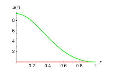
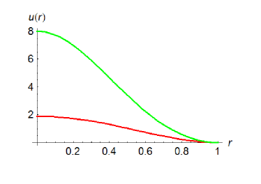
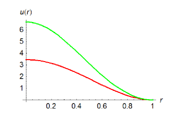
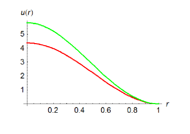
Figure 1: Radial solutions corresponding to Dirichlet boundary conditions calculated as explained in the text. Red line: minimum solution. Green line: mountain pass solution. Panel 1: $\lambda=0$. Panel 1: $\lambda=100$. Panel 1: $\lambda=150$. Panel 1: $\lambda=165$.

Now we move back to differential equation (3.1) but this time subjected to homogeneous Navier boundary conditions. We start as above, with the equation

$$w^{\prime\prime}-\frac{1}{r}\,w^{\prime}=\frac{1}{2}\,\frac{w^{2}}{r^{2}}+\frac{1}{2}\,\lambda\,r^{2},$$ (4.3)

and $w(1)=w^{\prime}(1)$ arbitrary, what corresponds to homogeneous Navier boundary conditions.

Also in this case we have employed a fourth-order Runge-Kutta method. The results of the numerical experiments are plotted in figure 2. They run in parallel to the results of the Dirichlet case. We have considered the Navier problem again for $r\in[0,1]$ and we have searched for solutions such that $\lim_{\epsilon\to 0^{+}}\,w(\epsilon)/\epsilon=0$, which corresponds to the extremum condition $u^{\prime}=0$ for the original differential equation. Using this shooting method we have found two different solutions which fulfill these requirements. One observes that for $\lambda=0$ there are one trivial and one non-trivial solutions. For $0<\lambda<\lambda_{c}$ there are two non-trivial solutions which approach each other for increasing $\lambda$. For $\lambda>\lambda_{c}$ no more solutions were numerically found. The critical value of $\lambda$ was numerically estimated to be $\lambda_{c}\approx 11.34$. Again, the smaller solution corresponds to a minimum of the “energy” functional and the larger solution corresponds to a mountain pass critical point. In all cases the minimum solution is strictly smaller than the mountain pass solution for all $0\leq r<1$.

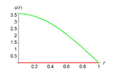
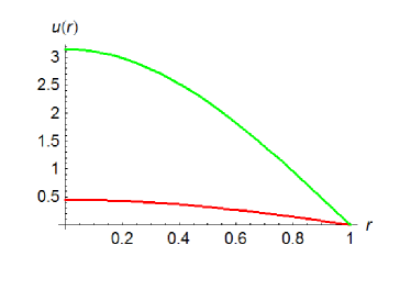
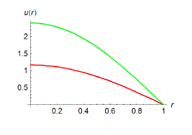
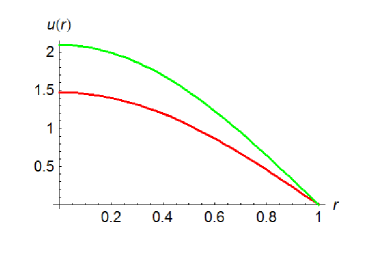
Figure 2: Radial solutions corresponding to Navier boundary conditions calculated as explained in the text. Red line: minimum solution. Green line: mountain pass solution. Panel 2: $\lambda=0$. Panel 2: $\lambda=5$. Panel 2: $\lambda=10$. Panel 2: $\lambda=11$.

5 Conclusions and Outlook

We have analyzed a differential equation appearing in the physical theory of epitaxial growth. We have started formally introducing the corresponding partial differential equation and then we have focused on radial solutions to its stationary counterpart. The resulting equation has been posed in the unit disk in the plane subjected to two different sets of boundary conditions. We have proven the existence of at least two solutions to both boundary value problems for small enough data. In each problem we have observed both solutions numerically and identified one of them with the local minimum of our “energy” functional and the other one with a mountain pass critical point. Due to the qualitatively similar results in both cases, the following assertions, and in particular the conjectures, refer to both boundary value problems. Our numerical simulations have revealed that the solutions are ordered in the sense that the one corresponding to the minimum lies strictly below (except for the boundary point $r=1$) the one corresponding to the mountain pass critical point. We have found the mountain pass solution is nontrivial for $0\leq\lambda<\lambda_{c}$ and the minimum solution is nontrivial for $0<\lambda<\lambda_{c}$ and trivial for $\lambda=0$. We have also proven nonexistence of solutions for large values of this parameter and we have found rigorous bounds for the size of the data separating existence from nonexistence, but the proofs will be reported elsewhere [12].

We conjecture the solution corresponding to the minimum is dynamically stable: if we considered the full evolution problem we would find this solution is locally stable for it. We also conjecture the mountain pass solution is dynamically unstable. We have numerically observed both solutions become closer for $\lambda$ approaching the critical value separating existence from nonexistence, so we conjecture that the transition from existence to nonexistence as we vary the parameter $\lambda$ is a saddle-node bifurcation for the corresponding evolution problem. We finally conjecture there exists a unique solution, that is dynamically unstable, for the critical value of $\lambda$, precisely the one that corresponds to the bifurcation threshold.

On the physical side, our results can be interpreted within the theory of nonequilibrium potentials [24]. The evolution problems correspond to gradient flows pursuing the minimization of our “energy” functionals, that play the role of nonequilibrium potentials. If both forcing term and initial condition are small the system will evolve towards the equilibrium state. If the forcing were stochastic the equilibrium state would become metastable. For a large forcing term there are no equilibrium states, so the system will keep on evolving forever in a genuine nonequilibrium fashion. In the theory of nonequilibrium growth, in which the forcing is normally assumed stochastic, it is known that these features affect both morphology and dynamics of the evolving interface [5]. In the case of existence of a local minimum this would imply in turn the existence of transient behavior, as found in different models of epitaxial growth [15]. Nonexistence of this state would mean that the asymptotic state is rapidly achieved. Residence times could be estimated with the help of the theory of nonequilibrium potentials [24]. Our results constitute a first step towards the understanding of these phenomena, although more work is needed in order to get a full understanding of them.

References

- [1] B. Abdellaoui, A. Dall’Aglio, and I. Peral, Some remarks on elliptic problems with critical growth in the gradient, J. Diff. Eq. 222 (2006) 21–62.
- [2] B. Abdellaoui, A. Dall’Aglio, and I. Peral, Regularity and nonuniqueness results for parabolic problems arising in some physical models, having natural growth in the gradient, J. Math. Pures Appl. 90 (2008) 242–269.
- [3] A. Ambrosetti and P. H. Rabinowitz, Dual variational methods in critical point theory and applications, J. Functional Analysis 14 (1973) 349–381.
- [4] B. Andrews, Gauss curvature flow: the fate of the rolling stones, Inventiones Mathematicae 138 (1999) 151–161.
- [5] A.-L. Barabási and H. E. Stanley, Fractal Concepts in Surface Growth (Cambridge University Press, Cambridge, 1995).
- [6] B. Chow, On Harnack’s inequality and entropy for the Gaussian curvature flow, Comm. Pure Appl. Math. 44 (1991) 469–483.
- [7] D. Blömker, F. Flandoli, and M. Romito, Markovianity and ergodicity for a surface growth PDE, Ann. Probab. 37 (2009) 275–313.
- [8] D. Blömker and M. Romito, Regularity and blow-up in a surface growth model, Dyn. Partial Differ. Equ. 6 (2009) 227–252.
- [9] D. Blömker and M. Romito, Local existence and uniqueness in the largest critical space for a surface growth model, preprint (2010).
- [10] I. Ekeland, On the variational principle, J. Math. Anal. Appl. 47 (1974) 324–353.
- [11] C. Escudero, Geometric principles of surface growth, Phys. Rev. Lett. 101 (2008) 196102.
- [12] C. Escudero, R. Hakl, I. Peral, and P. J. Torres, preprint.
- [13] J. García Azorero and I. Peral, Multiplicity of solutions for elliptics problems with critical exponents or with a non-symmetric term, Transactions of the American Mathematical Society 323 (1991) 877–895.
- [14] T. Halpin-Healy and Y.-C. Zhang, Kinetic Roughening, Stochastic Growth, Directed Polymers & all that, Phys. Rep. 254 (1995) 215–415.
- [15] C. A. Haselwandter and D. D. Vvedensky, Multiscale theory of fluctuating interfaces: renormalization of atomistic models, Phys. Rev. Lett. 98 (2007) 046102.
- [16] P. Hornung, Euler-Lagrange equation and regularity for flat minimizers of the Willmore functional, Comm. Pure Appl. Math. 64 (2011) 367–441.
- [17] M. Kardar, G. Parisi, and Y.-C. Zhang, Dynamic scaling of growing interfaces, Phys. Rev. Lett. 56 (1986) 889–892.
- [18] Z.-W. Lai and S. Das Sarma, Kinetic growth with surface relaxation: Continuum versus atomistic models, Phys. Rev. Lett. 66 (1991) 2348–2351.
- [19] G. Lengel, R. J. Phaneuf, E. D. Williams, S. Das Sarma, W. Beard, and F. G. Johnson, Nonuniversality in mound formation during semiconductor growth, Phys. Rev. B 60 (1999) R8469–R8472.
- [20] M. Marsili, A. Maritan, F. Toigo, and J. R. Banavar, Stochastic growth equations and reparametrization invariance, Rev. Mod. Phys. 68 (1996) 963–983.
- [21] T. Sun, H. Guo, and M. Grant, Dynamics of driven interfaces with a conservation law, Phys. Rev. A 40 (1989) R6763–R6766.
- [22] J. Villain, Continuum models of crystal growth from atomic beams with and without desorption, J. Phys. I (France) 1 (1991) 19–42.
- [23] T. J. Willmore, A survey on Willmore immersions, Geometry and Topology of Submanifolds, IV (Leuven, 1991), World Sci. (1992) pp. 11–16.
- [24] H. S. Wio and R. R. Deza, Aspects of stochastic resonance in reaction-diffusion systems: The nonequilibrium-potential approach, Eur. Phys. J. Special Topics 146 (2007) 111–126.