Brownian Net with Killing

Abstract. Motivated by its relevance for the study of perturbations of one-dimensional voter models, including stochastic Potts models at low temperature, we consider diffusively rescaled coalescing random walks with branching and killing. Our main result is convergence to a new continuum process, in which the random space-time paths of the Sun-Swart Brownian net are terminated at a Poisson cloud of killing points. We also prove existence of a percolation transition as the killing rate varies. Key issues for convergence are the relations of the discrete model killing points and their intensity measure to the continuum counterparts.

1 Introduction

The model. In the present paper, we consider the natural scaling limit of a generalization of the one-dimensional oriented percolation model, as introduced in [MNR13]. The model is parametrized by two non-negative numbers $b,k\geq 0$ and can defined as followed. Let us consider

$$\mathbb{Z}_{even}^{2}=\{(x,t)\in{\mathbb{Z}}^{2}\ :x+t\ \mbox{is even}\},$$ (1.1)

where $x$ is interpreted as a space coordinate and $t$ as a time coordinate. Each site $v=(x,t)\in\mathbb{Z}_{even}^{2}$ has two nearest neighbors with higher time coordinates: $v_{r}=(x+1,t+1)$ and $v_{l}=(x-1,t+1)$. $v$ is then randomly (and independently for different $v$’s) connected to a subset of its neighbors $v_{r}$ and $v_{l}$ by drawing arrows according to the following distribution.

• with probability $b$, draw the two arrows $(v\rightarrow v_{r})$ and $(v\rightarrow v_{l})$;

• do not draw any arrow with probability $k$, in which case it is called a killing point;

• with the remaining probability, draw a single arrow, its direction being chosen uniformly at random (see Figure 2).

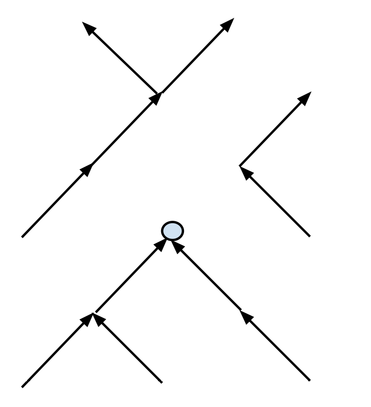
Figure 1: BCK (Branching, Coalescing, Killing) configuration.

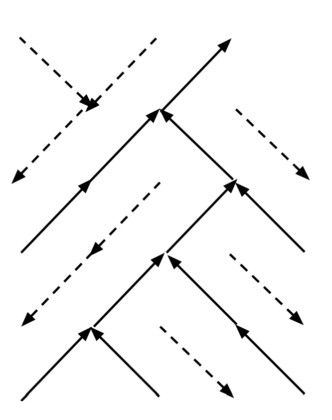
Figure 2: Construction of the dual of the discrete web.

If we denote by ${\cal E}^{b,k}$ the resulting random arrow configuration, the random directed graph ${\cal G}^{b,k}=(\mathbb{Z}_{even}^{2},{\cal E}^{b,k})$ defines a certain type of one dimensional percolation model oriented forward in the $t$-direction. By definition, a path $\pi$ along ${\cal E}^{b,k}$ will denote a path starting from any site of ${\mathbb{Z}}_{even}^{2}$ and following the random arrow configuration until getting killed (by reaching a killing point) or reaching $\infty$. More precisely, a path $\pi$ is the graph of a function defined on an interval in ${\mathbb{R}}$ of the form $[\sigma_{\pi},e_{\pi})$, with $\sigma_{\pi},e_{\pi}\in{\mathbb{Z}}\cup\{\infty\}$ such that $e_{\pi}=\infty$ or else $(\pi(e_{\pi}),e_{\pi})$ is a killing point; for every integer $t\in[\sigma_{\pi},e_{\pi})$, $(\pi(t),t)$ connects to $(\pi(t+1),t+1)$ and $\pi$ is linear between $t$ and $t+1$.

Considering the set of all the paths along ${\cal E}^{b,k}$, one generates an infinite family ${\cal U}^{b,k}$ that can loosely be described as a collection of graphs of one dimensional coalescing simple random walks that branch with probability $b$ and are killed with probability $k$. A walk at space-time site $v$ can create two new walks (starting respectively at $v_{l}$ and $v_{r}$) with probability $b$ and can be killed with probability $k$; two walks move independently when they are apart but become perfectly correlated (i.e., they coalesce) upon meeting at a space-time point. In the following, ${\cal U}^{b,k}$ will be referred to as a system of branching-coalescing-killing random walks (or in short, BCK) with parameters $(b,k)$.

This model encompasses several classical models from statistical mechanics. For $p\in(0,1)$ and $b=p^{2}$, $k=(1-p)^{2}$, one recovers the standard one dimensional oriented percolation model. When $b=k=0$, the trajectories in our random graphs are distributed as coalescing random walks. In the present work, we will investigate the behavior of this model when the parameters $b$ and $k$ are non-zero, but small. This generalizes previous work by Sun and Swart [SS08], and by the present authors [NRS10], where the case $k=0$ and small $b$ was investigated.

Motivations. Our interest stems from several applications in interacting particle systems. On the one hand, it is well known that the classical voter model is dual to coalescing random walks. On the other hand, Cox, Durrett and Perkins [CDP11] noticed that several models in ecology — the spacial Lokta-Volterra model [NP99], the evolution of cooperation [OHLN06] — and in statistical mechanics — non linear voter models [MoDDGL99] but also the stochastic Potts model in $d=1$, see [MNR13] — can be seen as perturbations (of strength $\epsilon$) of the voter model in a certain range of their parameter space. More precisely, they noticed that in a certain range of the transition rates, those models can be written in the form

$$\forall j\in\{1,\cdots,q\},\ \ c_{j}^{\epsilon}(\eta,x)\ =\ c_{j}^{v}(\eta,x)+c_{j}^{*,\epsilon}(\eta,x)$$ (1.2)

where $c^{\epsilon}_{j}(\eta,x)$ is the transition rate of site $x$ to state $j$ given a configuration $\eta$, $c_{j}^{v}$ is the transition rate of a standard (possibly non nearest neighbor) voter model and the remaining term is such that $c_{j}^{*,\epsilon}(\eta,x)\rightarrow 0$ as $\epsilon\rightarrow 0$.

In general, the interacting particle systems alluded to above are difficult to study either because of a lack of monotonicity (Lotka-Volterra model) or because of the intrinsic complexity of the model (certain models of evolution of cooperation). Since the voter model is well understood, the idea is to use standard results about that model to derive some properties (such as coexistence of species in the Lokta Voterra model) of the more complex models described above. This program was carried out successfully in [CDP11], where it is shown that for $d\geq 3$, the properly rescaled local density of particles converges to the solution of a reaction diffusion equation, and that properties of the underlying particle system can be derived from the behavior of this PDE.

The present work is a first step to understand the situation in low dimension, when $d=1$. The idea is the following. Since the voter model is dual to coalescing random walks, perturbation of the voter model should be dual to perturbation of coalescing random walks. As a consequence, it is natural to consider a system of coalescing random walks with an additional perturbative branching and killing mechanism. In fact, in a future work [NRS13], it will be shown that very general perturbations of voter models in dimension 1 converge to a continuum object which is constructed via the scaling limit of the BCK: an object that we name the Brownian net with killing and which is the central object of this work.

Scaling of the parameters. As we shall see below (see Theorem 1.1), the Brownian net with killing emerges as the scaling limit of the BCK model when the branching and killing parameters are scaled differently. More precisely, if we denote $k_{\beta}$ and $b_{\beta}$ the killing and branching parameters of the model, then if $b_{\beta}=e^{-\beta}b$ and $k_{\beta}=e^{-2\beta}k$ for some $b,k\geq 0$, the (properly rescaled) BCK converges to the Brownian net with killing as $\beta\rightarrow\infty$.

Although scaling branching and killing differently might appear quite artificial at first sight, we will show in [NRS13] that such scaling appears naturally in statistical mechanics. In particular, when considering the stochastic Potts model in one dimension, we will show that at large inverse temperature $\beta$, such a model is asymptotically dual to the BCK with branching and killing parameters

$$b_{\beta}=\frac{q}{2}e^{-\beta}\ \ \ k_{\beta}=qe^{-2\beta},$$

where $q$ is the number of colors in the system. For this reason, we will parametrize the BCK with $\beta$ and interpret this number as the inverse temperature of the model.

Main results. To illustrate our approach, let us first consider the case $b=k=0$. For every $(x,t)\in{\mathbb{Z}}_{even}^{2}$, let us denote by $\pi_{x,t}$ the unique path starting from the spacial point $x$ at time $t$ and following the random arrow configuration up to $\infty$. As mentioned earlier, this path is simply the graph of a simple symmetric random walk. Furthermore, the paths starting from different locations $(x_{i},t_{i})$ are coalescing, i.e. they move independently and then coalesce upon meeting at any space time point.

Let $n\in{\mathbb{N}}$ and let $\{(x_{i},t_{i})\}_{i\leq n}$ be $n$ points in ${\mathbb{Z}}_{even}^{2}$. If one rescales space and time diffusively by the transformation

$$S_{\beta}(x,t)\ =(xe^{-\beta},te^{-2\beta}),$$ (1.3)

it is then easy to see that if $\{(x_{i}^{\beta},t_{i}^{\beta})\in{\mathbb{Z}}_{even}^{2}\}_{\beta}$ are such that

$$\forall i\leq n,\lim_{\beta\uparrow\infty}\ \ S_{\beta}(x_{\beta}^{i},t_{\beta}^{i})\rightarrow(x^{i},t^{i}),$$

then the family of rescaled paths $\{S_{\beta}\left(\pi_{(x_{i}^{\beta},t_{i}^{\beta})}\right)\}$ converges to a family of graphs of $n$ coalescing one dimensional Brownian motions starting from the space-time points $\{(x_{i},t_{i})\}$ — see Tòth and Werner [TW98] and Arratia [A81]. In [FINR04], Fontes, Newman, Isopi and Ravishankar strengthened this statement by proving that the set of all paths in the random configuration (also called the discrete web) converges to a continuum object that they called the Brownian web (BW).

In Section 2.1 below, we will precisely define the probability space on which the Brownian web lives, as it was introduced in [FINR04]. For the sake of presentation, we start with an informal discussion (see also Fig. 3). The Brownian web is a random collection of continuous paths with specified starting points and ending points in space-time. The paths take values in a metric space $(\bar{\mathbb{R}}^{2},\rho)$ which is a compactification of ${\mathbb{R}}^{2}$. $(\Pi,d)$ denotes the space whose elements are paths with specific starting points and ending points. The metric $d$ is then defined as the maximum of the sup norm of the distance between two paths, the distance between their respective starting points and the distance between their ending points. (In particular, when no killing occurs, as in the discrete and Brownian webs, the ending point of each path is $\infty$). The Brownian web takes values in the metric space $({\cal H},d_{\cal H})$, whose elements are compact collection of paths in $(\Pi,d)$ with $d_{\cal H}$ being the induced Hausdorff metric. Thus the Brownian web is an $({\cal H},{\cal F}_{\cal H})$-valued random variable, where ${\cal F}_{\cal H}$ is the Borel $\sigma$-field associated to the metric $d_{\cal H}$.

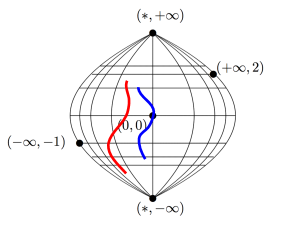
Figure 3: Informally, the distance between two paths is obtained by first mapping the two paths into a compact subset of the plane (blue and red curves) and then taking the distance between the images.

In  [FINR04], the authors define the the Brownian web as the scaling limit of the discrete web. More precisely, it is shown that there exists a random variable $\cal W$ on $({\cal H},d_{\cal H})$ — the Brownian web — such that

$$S_{\beta}(W)\rightarrow{\cal W}\ \ \mbox{in law,}$$

where $W$ denotes the discrete web. Building on their approach, we will show an analogous result for the BCK when $b,k$ are nonzero:

Theorem 1.1.

Let $b,k\geq 0$ and $\lim_{\beta\uparrow\infty}k_{\beta}e^{2\beta}=k$, $\lim_{\beta\uparrow\infty}b_{\beta}e^{\beta}=b$. There exists a random variable ${\cal N}^{b,k}$ taking values in $({\cal H},{\cal F}_{\cal H})$ so that

$$S_{\beta}({\cal U}^{b_{\beta},k_{\beta}})\ \rightarrow\ {\cal N}^{b,k}\ \ \ \ \text{in law.}$$

In the following, we will say that ${\cal N}^{b,k}$ percolates (more accurately we should say “percolates from the origin”) if there exists a path in ${\cal N}^{b,k}$ starting from the origin and reaching to $\infty$. The following result is a continuum analog of a result proved for the discrete BCK in [MNR13].

Theorem 1.2.

1. $\mathcal{N}^{b,k}$ is identical in law with $S_{\ln(b)}({\cal N}^{1,k/b^{2}})$.

2. There exists $k_{c}\in(0,\infty)$ such that

   • for every $k<k_{c}$, ${\mathbb{P}}(\mathcal{N}^{1,k}\ \mbox{ percolates})>0$.

   • for every $k>k_{c}$, ${\mathbb{P}}(\mathcal{N}^{1,k}\ \mbox{ percolates})=0$.

Remark 1.3.

Note that the convergence result, Theorem 1.1 immediately implies the scaling property

$$S_{\ln(b)}(\mathcal{N}^{b,k})\ =\ \mathcal{N}^{1,\frac{k}{b^{2}}}\ \ \mbox{in law}.$$

Indeed, for $e^{\beta}b_{\beta}\rightarrow b$ and $e^{2\beta}k_{\beta}\rightarrow k$, we have

$$S_{\beta+\ln(b)}({\cal U}^{b_{\beta},k_{\beta}})\rightarrow\mathcal{N}^{1,\frac{k}{b^{2}}},$$

whereas

$$S_{\beta+\ln(b)}({\cal U}^{b_{\beta},k_{\beta}})=S_{\ln(b)}\circ S_{\beta}({\cal U}^{b_{\beta},k_{\beta}})\rightarrow S_{\ln(b)}(\mathcal{N}^{b,k}).$$

Outline. The rest of the paper is organized as follows. In Section 2, we give two alternative constructions of the Brownian net with killing. In Section 3, we prove the percolation property of the killed Brownian net stated in Theorem 1.2. Finally, in Section 4, we show that the BCK converges (under proper rescaling) to the Brownian net with killing, as stated in Theorem 1.1. A key issue in proving that convergence, as discussed at the beginning of Section 4 and then treated in Sections 4.1 and 4.2, is the convergence of the Poissonian killing points in such a way that if a continuum path is killed somewhere, then the discrete approximating paths are killed as well.

2 Construction of the Brownian Net with Killing

In this section, we give two alternative constructions of the object $\mathcal{N}^{b,k}$. We first briefly outline the ideas behind those two constructions.

One web, two markings. In a first approach, in the spirit of [NRS10], we start by describing the scaling limit in the special case $b=k=0$. In this particular setting, where the branching and killing parameters are turned off, the discrete BCK becomes an infinite family of coalescing random walks, also referred to as a discrete web — see [FINR04].

As we shall see in Section 2.2, the Brownian web can be used to construct the natural scaling limit for the BCK, the Brownian net with killing $\mathcal{N}^{b,k}$ in the case where $b,k\neq 0$. At the discrete level, the idea is simple and relies on the idea that the BCK can be constructed by starting with a discrete web and then turn on the killing and branching parameters. Effectively, one starts with a discrete web, and then independently at each site

• removes an arrow with probability $k$.

• or adds an extra arrow with probability $b$.

In Section 2.2.3, we will explain how one can generalize this construction to the continuum level. More precisly, we will identify some geometrical random configurations in the Brownian Web, playing a role analogous to the arrows of the discrete web (the BCK with no branching or killing). Finally, we will briefly explain how those “continuum arrows” can be added or removed by two Poissonian markings in order to generate the Brownian net with killing $\mathcal{N}^{b,k}$ from the Brownian web ${\cal W}$.

One net, one marking. Alternatively, our second construction (presented in Section 2.3) will only make use of a single set of marks, while using a richer underlying structure: the standard Brownian net (with no killing), an object introduced using different methods by Sun and Swart [SS08] and analysed by Newman, Ravishankar and Schertzer [NRS10]. In Section 2.3.1, we first present the three distinct direct constructions of the standard Brownian net, due to Sun and Swart. In Section 2.3.4, we will show how one can directly construct the killed Brownian net from the standard Brownian net by adding one extra set of marks. This direct construction will be based on some intermediate results provided in Sections 2.3.2 and 2.3.3. We note that those will also be relevant for other parts of this paper. In Section 2.3.2, we give some results about the special points of the Brownian net. In Section 2.3.3, we introduce the branching-coalescing point set of the standard Brownian net.

Finally, in Section 2.4, the equivalence between our two alternative constructions of the killed Brownian net is established.

2.1 The Space $({\cal H},d_{\cal H})$

As in [FINR04], we will define the Brownian net with killing as a random compact set of paths. In this section, we briefly outline the construction of the space of compact sets. For more details, the interested reader may refer to [FINR04].

First define $(\bar{\mathbb{R}}^{2},\rho)$ to be the compactification of ${\mathbb{R}}^{2}$ with

$$\rho((x_{1},t_{1}),(x_{2},t_{2}))\ =\ |\phi(x_{1},t_{1})-\phi(x_{2},t_{2})|\vee|\psi(t_{1})-\psi(t_{2})|,$$

where

$$\phi(x,t)=\frac{\tanh(x)}{1+|t|}\ \ \ \mbox{and}\ \ \ \psi(t)=\tanh(t).$$

In particular, we note that the mapping $(x,t)\rightarrow(\phi(x,t),\psi(t))$ maps $\bar{\mathbb{R}}^{2}$ onto a compact subset of ${\mathbb{R}}^{2}$.

Next, let $C[t_{0},t_{1}]$ denote the set of continuous functions from $[t_{0},t_{1}]$ to $[-\infty,+\infty]$. From there, we define the set of continuous paths in ${\mathbb{R}}^{2}$ (with a prescribed starting and ending point) as

$$\Pi:=\cup_{t_{0}\leq t_{1}}C[t_{0},t_{1}]\times\{t_{0}\}\times\{t_{1}\}.$$

Finally, we equip this set of paths with a metric $d$, defined as the maximum of the sup norm of the distance between two paths, the distance between their respective starting points and the distance between their ending points. (In particular, when no killing occurs, as in the forward Brownian web, the ending point of each path is $\infty$). More precisely, if for any path $\pi$, we denote by $\sigma_{\pi}$ the starting time of $\pi$ and by $e_{\pi}$ its ending time, we have

$$d(\pi_{1},\pi_{2})\ =\ |\psi(\sigma_{\pi_{1}})-\psi(\sigma_{\pi_{2}})|\vee|\psi(e_{\pi_{1}})-\psi(e_{\pi_{2}})|\vee\max_{t}\ \rho((\bar{\pi}_{1}(t),t),(\bar{\pi}_{2}(t),t)),$$

where $\bar{\pi}$ is the extension of $\pi$ into a path from $-\infty$ to $+\infty$ by setting

$$\bar{\pi}(t)=\left\{\begin{array}[]{c}\pi(\sigma_{\pi})\ \ \mbox{for $t<\sigma_{\pi}$},\\ \pi(e_{\pi})\ \ \mbox{for $t>e_{\pi}$.}\end{array}\right.$$

Finally, let ${\cal H}$ denote the set of compact subsets of $({\cal H},d_{\cal H})$ where $d_{\cal H}$ is the Hausdorff metric

$$d_{\cal H}(K_{1},K_{2})=\max_{\pi_{1}\in K_{1}}\min_{\pi_{2}\in K_{2}}d_{\cal H}(\pi_{1},\pi_{2})\vee\max_{\pi_{2}\in K_{2}}\min_{\pi_{1}\in K_{1}}d_{\cal H}(\pi_{1},\pi_{2}).$$

In [FINR04], it is proved that $({\cal H},d_{\cal H})$ is Polish. In the following, we will construct the Brownian net with killing as a random element of this space.

2.2 One Web, Two Markings

2.2.1 The Brownian Web

As mentioned in the introduction, the Brownian web is the scaling limit of the discrete web under diffusive space-time scaling and is defined as a random element of $({\cal H},d_{\cal H})$. The next theorem, taken from [FINR04], gives some of the key properties of the BW.

Theorem 2.1.

There is an $({\cal H},{\cal F}_{{\cal H}})$-valued random variable ${{\cal W}}$ whose distribution is uniquely determined by the following three properties.

• from any deterministic point $(x,t)$ in ${\mathbb{R}}^{2}$, there is almost surely a unique path ${B}_{(x,t)}$ starting from $(x,t)$.

• for any deterministic, dense countable subset ${\cal D}$ of ${\mathbb{R}}^{2}$, almost surely, ${{\cal W}}$ is the closure in $(\Pi,d)$ of $\{{B}_{(x,t)}:(x,t)\in{\cal D}\}.$

• for any deterministic $n$ and $(x_{1},t_{1}),\ldots,(x_{n},t_{n})$, the joint distribution of ${B}_{(x_{1},t_{1})},\ldots,{B}_{(x_{n},t_{n})}$ is that of coalescing Brownian motions from those starting points (with unit diffusion constant).

Note that (i) provides a practical construction of the Brownian web. For $\cal D$ as defined above, construct coalescing Brownian motion paths starting from $\cal D$. This defines a skeleton for the Brownian web that is denoted by ${\cal W}({\cal D})$. ${\cal W}$ is simply defined as the closure of this precompact set of paths.

2.2.2 The Backward (Dual) Brownian Web

The discrete web is defined on ${\mathbb{Z}}_{even}^{2}$ and oriented forward in time. There is a natural dual system of paths defined on the complementary lattice ${\mathbb{Z}}_{odd}^{2}:=\{(x,t)\ :\ x+t\ \ \mbox{is odd}\}$ and oriented in the reverse direction. Indeed, given a realization of $W$, at any vertex $(x,t)\in{\mathbb{Z}}_{odd}^{2}$, we can construct a (backward) arrow configuration by rotating the (forward) arrow at $(x,t-1)\in\mathbb{Z}_{even}^{2}$ through $180^{\circ}$ and then translating its starting point to $(x,t)$ (see Fig. 2). This defines a system of coalescing random walks starting from ${\mathbb{Z}}_{odd}^{2}$, running backward in time without crossing the forward discrete web paths. Furthermore, the resulting system of paths is easily seen to be identically distributed with the original model, after a $180^{\circ}$ rotation followed by a unit translation in the $x$ or $t$ direction.

This family will be referred to as the backward discrete web, and the backward (dual) BW $\hat{\mathcal{W}}$ may be defined analogously as a functional of the (forward) BW $\mathcal{W}$. More precisely for a countable dense deterministic set of space-time points, the backward BW path from each of these is the (almost surely) unique continuous curve (going backwards in time) from that point that does not cross (but may touch) any of the (forward) BW paths; $\hat{\mathcal{W}}$ is then the closure of that collection of paths. The first part of the next proposition states that the “double BW”, i.e., the pair $(\mathcal{W},\hat{\mathcal{W}})$, is the diffusive scaling limit of the corresponding discrete pair $(W,\hat{W})$ (after diffusive scaling and as the scale parameter $\beta\to\infty$). Convergence in the sense of weak convergence of probability measures on $({\cal H},{\cal F}_{\cal H})\times(\hat{\cal H},\hat{\cal F}_{\cal H})$ was proved in [FINR04]; convergence of finite dimensional distributions and the second part of the proposition were already contained in [TW98].

Proposition 2.2.

1. Up to a reflection with respect to the $x$-axis, ${\cal W}$ and $\hat{\cal W}$ are identically distributed.

2. Invariance principle : $\left(S_{\epsilon}(W),S_{\epsilon}(\hat{W})\right)\to(\mathcal{W},\hat{\mathcal{W}})$ as $\epsilon\to 0$.

3. For any (deterministic) pair of points $(x,t)$ and $(\hat{x},\hat{t})$ there is almost surely a unique forward path $B$ starting from $(x,t)$ and a unique backward path $\hat{B}$ starting from $(\hat{x},\hat{t})$.

The next proposition, cited from [STW00], which gives the joint distribution of a single forward and single backward BW path, has an extension to the joint distribution of finitely many forward and backward paths. We remark that that extension can be used to give a characterization (or construction) of the double Brownian web $({\cal W},\hat{\cal W})$ analogous to the one for the (forward) BW from Theorem 2.1 — see [STW00, FINR05] for more details.

Proposition 2.3.

1. Distribution of $(B,\hat{B})$: Let $(B_{ind},\hat{B}_{ind})$ be a pair of independent forward and backward Brownian motions starting at $(x,t)$ and $(\hat{x},\hat{t})$ and let $(R_{\hat{B}_{ind}}(B_{ind}),\hat{B}_{ind})$ be the pair obtained after reflecting (in the Skorohod sense) $B_{ind}$ on $\hat{B}_{ind}$, i.e., $R_{\hat{B}_{ind}}(B_{ind})$ is the following function of $u\in[t,\hat{t}]$:

   $$R_{\hat{B}_{ind}}(B_{ind})=\left\{\begin{array}[]{ll}B_{ind}(u)-0\wedge\min_{t\leq v\leq u}(B_{ind}(v)-\hat{B}_{ind}(v))\ \ \ \ \textrm{on $\{B_{ind}(t)\geq\hat{B}_{ind}(t)\}$},\\ B_{ind}(u)-0\vee\max_{t\leq v\leq u}(B_{ind}(v)-\hat{B}_{ind}(v))\ \ \ \ \textrm{on $\{B_{ind}(t)<\hat{B}_{ind}(t)\}$}.\end{array}\right.$$ (2.4)

   Then

   $$(R_{\hat{B}_{ind}}(B_{ind}),\hat{B}_{ind})=(B,\hat{B})\ \ \textrm{in law},$$ (2.5)

   where $B$ is the path in ${\cal W}$ starting at $(x,t)$ and $\hat{B}$ is the path in $\hat{W}$ starting at $(\hat{x},\hat{t})$.

2. Similarly,

   $$(B_{ind},R_{B_{ind}}(\hat{B}_{ind}))=(B,\hat{B})\ \ \textrm{in law}.$$ (2.6)

2.2.3 Special Points of the Brownian Web

While there is only a single path starting from (and no path passing through) any deterministic point in ${\mathbb{R}}^{2}$ in both the forward and backward webs, there exist random points $z\in{\mathbb{R}}^{2}$ with one or more than one path passing through or starting from $z$. As we shall see later, those “special points” of the Brownian web will play a key role in our construction of the Brownian net with killing. We remark that here when we say that a path starts from $(x_{0},t_{0})$, it does not preclude the possibility that it is the $t\geq t_{0}$ continuation of a path that passes through $(x_{0},t_{0})$.

We start by describing the “types” of points $(x,t)\in{\mathbb{R}}^{2}$, whether deterministic or not. We say that two paths $B,B^{\prime}\in{\cal W}$ are equivalent paths entering $z=(x,t)$, denoted by

$$B=_{in}^{z}B^{\prime}$$ (2.7)

iff $B=B^{\prime}$ on $[t-\epsilon,t]$ for some $\epsilon>0$. The relation $=^{z}_{in}$ is a.s. an equivalence relation on the set of paths in ${\cal W}$ entering the point $z$ and we define $m_{in}(z)$ as the number of those equivalence classes. ($m_{in}(z)=0$ if there are no paths entering $z$.) $m_{out}(z)$ is defined as the number of distinct paths starting from $z$. For $\hat{\cal W}$, $\hat{m}_{in}(z)$ and $\hat{m}_{out}(z)$ are defined similarly.

Definition 2.1.

The type of $z$ is the pair $(m_{in}(z),m_{out}(z))$.

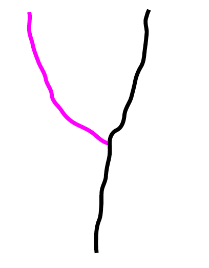
Figure 4: A schematic diagram of a right $(m_{\mbox{{\scriptsize\emph{in}}}},m_{\mbox{{\scriptsize\emph{out}}}})=(1,2)$ point. In this example the incoming forward path connects to the rightmost outgoing path (with a corresponding dual connectivity for the backward paths), the left outgoing path is a newly born path.

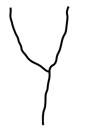
Figure 5: A branching point is created by attaching the left branch to the incoming path.

The following results from [TW98] (see also  [FINR05]) specify what types of points are possible in the Brownian web.

Theorem 2.4.

For the Brownian web, almost surely, every $(x,t)$ is one of the following types, all of which occur: $(0,1)$, $(0,2)$, $(0,3)$, $(1,1)$, $(1,2)$, $(2,1)$.

Proposition 2.5.

Let $t$ be a deterministic time. Almost surely for every realization of the Brownian web, any point of the form $(x,t)$ (with $x$ deterministic or random) is either of type $(0,1)$, $(1,1)$ or $(0,2)$.

Proposition 2.6.

For the Brownian web, almost surely for every $z$ in ${\mathbb{R}}^{2}$, $\hat{m}_{in}(z)=m_{out}(z)-1$ and $\hat{m}_{out}(z)=m_{in}(z)+1$.

Finally, we close this section by proving an easy lemma about the special points of the Brownian web. This result will be useful in the rest of the paper but can be skipped at first reading.

Lemma 2.1.

Let $w$ be a path in ${\cal W}$ starting from a point $z=(x,t)$. If $z$ is not a $(0,3)$ point, then there exists a sequence of paths $w_{n}\in{\cal W}$ starting strictly below time $t$ (i.e. with $\sigma_{w_{n}}<t$) and coalescing with $w$ at $\tau_{n}>t$, with $\tau_{n}\rightarrow t$.

Proof.

We first claim that if $z$ is not of type $(0,3)$, for any outgoing path, there exists a sequence $w_{n}$ starting below time $t$ such that $w_{n}\rightarrow w$ in the topology $(\Pi,d)$. By Theorem 2.4, we need to show that our result holds for points of the type $(*,1)$ and $(*,2)$ — where $*$ can be 0,1 or 2 when there is a single outgoing path, and $0$ or $1$ for two outgoing paths.

Let us first show that our claim holds when $z$ is of type $(*,1)$. Let us consider any sequence $w_{n}$ in ${\cal W}$ with starting point $z_{n}=(x_{n},\sigma_{w_{n}})\rightarrow z$ and $\sigma_{w_{n}}<t$. Since ${\cal W}$ is a compact set of paths, from any subsequence extracted from $w_{n}$, one can extract a further subsequence converging to a path starting from $z$. Since $w$ is the unique such path, we conclude that the sequence $w_{n}$ must converge to $w$. Let us now show that our claim holds for points of the type $(*,2)$. W.l.o.g. we aim to show that the left outgoing path can be approximated by a sequence $w_{n}$ with $\sigma_{w_{n}}<t$. Let $\hat{w}$ be the left-most backward path in $\hat{\cal W}$ starting from the point $z$ and let us consider a sequence $w_{n}$ starting in the left region delimited by $\hat{w}$. Since dual paths in $\hat{\cal W}$ do not cross paths in the forward web ${\cal W}$, $w_{n}$ hits the time line ${\mathbb{R}}\times\{t\}$ either strictly to the left of $z$ — i.e. at a point $(x_{n},t)$ such that $x_{n}<x$ — or at $z$. In order to see that the latter does not occur, we distinguish between two cases

1. $z$ is of type $(0,2)$. Since there is no incoming Brownian web path at $z$, our claim is obvious.

2. $z$ is of type $(1,2)$. Recall that we chose $\hat{w}$ to be the left-most backward path starting from $z$. For $(1,2)$ points, the incoming path is necessarily to the right of this backward path (squeezed between the left-most and the right-most backward paths), implying that $w_{n}$ can not coalesce with $w$ before time $t$ (the time coordinate of $z$). Hence if $w_{n}$ hits the point $z$, this would imply the existence of two non-equivalent paths entering $z$, which would contradict the definition of a $(1,*)$ point.

Since points of type $(*,2)$ are necessarily of one of the previous two types (again by Theorem 2.4), it follows that we must have $x_{n}<x$. This implies that $w_{n}$ coalesces with the left outgoing path before meeting the right outgoing path starting from $z$. By reasoning as for the $(*,1)$ case, this easily implies that $w_{n}$ must converge to the left outgoing path.

It remains to show that if $w_{n}$ converges to $w$ with $\sigma_{w_{n}}<t$, then $w_{n}$ must coalesce with $w$ at a time $\tau_{n}$, with $\tau_{n}\rightarrow t$. In order to see that, let us consider some arbitrary small $\epsilon>0$. In [FINR04], it is proved that the set of paths with starting time $\sigma_{w}\leq t$, hits the line ${\mathbb{R}}\times\{t+\epsilon\}$ at only locally finitely many points. Hence, $w_{n}(t+\epsilon)$ must be stationary after some rank, implying that $w_{n}(t+\epsilon)=w(t+\epsilon)$ and that $w_{n}$ must have coalesced with $w$ before time $t+\epsilon$. Since $\epsilon$ is arbitrarily small, this ends the proof of our lemma.

∎

2.2.4 Construction of the Brownian Net with Killing

In our construction of the Brownian net with killing, $(1,2)$ points and $(1,1)$ points will play a special role. First, it is important to realize that points of type $(1,2)$ can be characterized in two ways, both of which will play a crucial role in our construction of the Brownian net with killing. 1) By Proposition 2.6, $z\in{\mathbb{R}}^{2}$ is of type $(1,2)$ precisely if both a forward and a backward path pass through $z$. 2) A single incident path continues along exactly one of the two outward paths — with the choice determined intrinsically. It is either left-handed or right-handed according to whether the continuing path is to the left or to the right of the other outgoing path. For a left (resp., right) $(1,2)$ point $z$, the right (resp, left) outgoing path will be referred to as the newly born path starting from $z$. See Fig. 5 for a schematic diagram of the “right-handed” case.

In particular, one can add a “continuum” arrow at a given $(1,2)$ point $z$ by not only connecting an incoming path to the continuing outgoing path, but also to the newly born path starting from $z$ — see Fig. 5. In the discrete picture, this amounts to adding an arrow which induces a “macroscopic” effect in the web. This particular construction will be discussed later in this section.

On the other hand, a point of type $(1,1)$ can be seen as a single arrow passed through by a path, and whose suppression will induce a macroscopic effect on the Brownian web, i.e., the suppression of this arrow will disconnect this path into two large components.

As already mentioned at the beginning of this section, the discrete BCK can be constructed from the discrete web by randomly adding and removing arrows. Now that we have identified the random structures playing the role of arrows at the continuum level, we need to implement some random selection of those structures. This will be done by first defining two uniform measures on those sets of ”arrows”: one measure for the $(1,2)$ points — the local time measure, related to the intersection local time between the forward and backward paths of the Brownian web; see Proposition 2.8 below — and one for $(1,1)$ points — the time length measure; see Proposition 2.7.

Proposition 2.7 (Time Length Measure).

Given a realization of the Brownian web, for every Borel set $E\subset{\mathbb{R}}^{2}$, define

$${\cal T}_{web}(E)\ :=\ \int_{-\infty}^{\infty}\ |\{x\ :\ (x,t)\in E\cap(1,1)\}|dt,$$

where $(1,1)$ refers to the set of $(1,1)$ points of the Brownian web and $|\cdot|$ denotes cardinality. ${\cal T}_{web}$ defines a $\sigma$-finite measure on ${\mathbb{R}}^{2}$ so that for every $\pi\in{\cal W}$

$$\forall\ x_{1}<x_{2},t_{1}<t_{2},\ \ {\cal T}_{web}(\{(x,t)\in[x_{1},x_{2}]\times[t_{1},t_{2}]\ :\pi(t)=x\})\ =\ \int_{t_{1}\vee\sigma_{\pi}}^{t_{2}\vee\sigma_{\pi}}1_{\pi(t)\in[x_{1},x_{2}]}\ \ dt.$$ (2.8)

In other words, if one considers the set defined as the intersection of a rectangle with a Brownian web path, the time length measure of this set is given by the time spent by this path in the rectangle.

Proof.

It is straightforward to check that ${\cal T}_{web}$ defines a measure. To prove the $\sigma$-finite property, let us consider a dense countable deterministic set ${\cal D}:=\{z_{1},\cdots,z_{n},\cdots\}$ in ${\mathbb{R}}^{2}$, and define ${\cal D}_{n}=\{z_{1},\cdots,z_{n}\}$. In [FINR04] it was shown that for every path $\pi\in{\cal W}$ and every time $t$ such that $\sigma_{\pi}<t$, we must have $(\pi(t),t)\in{\cal W}({\cal D})$, where ${\cal W}({\cal D})$ refers temporarily to the trace of the skeleton ${\cal W}({\cal D})$. It follows that $(1,1)\subset{\cal W}({\cal D})$ and that

$${\cal T}_{web}(E) = \int_{-\infty}^{\infty}\ |\{x\ :\ (x,t)\in E\cap(1,1)\cap{\cal W}({\cal D})\}|dt$$

$$= \lim_{n\uparrow\infty}\int_{-\infty}^{\infty}\ |\{x\ :\ (x,t)\in E\cap(1,1)\cap{\cal W}({\cal D}_{n})\}|dt,$$

where the last identity follows from the monotone convergence theorem. Finally, since ${\cal W}({\cal D}_{n})$ meets any horizontal line ${\mathbb{R}}\times\{t\}$ at $n$ points at the most (recall that there is a.s. a unique path starting from any deterministic point ), this proves the $\sigma-$finite property for our measure.

It remains to show (2.8). For every realization of the Brownian web ${\cal W}$, let us consider the set of times

$$T=\{t\ :\ \exists\pi\in{\cal W}\ \ \mbox{with $\sigma_{\pi}<t$ and $(\pi(t),t)$ is not of type $(1,1)$}\ \}.$$

In [FINR04], [TW98], it was shown that for every deterministic time $t$, any point $(x,t)$, with $x\in{\mathbb{R}}$, is either of the type $(0,1)$, $(0,2)$ or $(1,1)$. Hence, at a determistic time $t$, any point $(x,t)$ such that there exists some $\pi\in{\cal W}$ with $\sigma_{\pi}<t$ so that $x=\pi(t)$ must be a $(1,1)$ point, which amounts to saying that $t$ does not belong to the set $T$ almost surely. By a direct application of the Fubini Theorem, the set of times which belongs to $T$ must have zero Lebesgue measure, implying that

$${\cal T}_{web}(\{(x,t)\in[x_{1},x_{2}]\times[t_{1},t_{2}]\ :\pi(t)=x\}) = \int_{t_{1}\vee\sigma_{\pi}}^{t_{2}\vee\sigma_{\pi}}1_{\pi(t)\in[x_{1},x_{2}]}1_{(\pi(t),t)\in(1,1)}\ \ dt$$

$$= \int_{t_{1}\vee\sigma_{\pi}}^{t_{2}\vee\sigma_{\pi}}1_{\pi(t)\in[x_{1},x_{2}]}\ \ dt,$$

where the first equality follows directly from the definition of ${\cal T}_{web}$.

∎

The following Proposition is cited from [SSS13].

Proposition 2.8 (Local Time Measure).

Almost surely for every realization of the Brownian web, there exists a unique $\sigma$-finite measure ${\cal L}$, concentrated on the set of points of type $(1,2)$ in ${\cal W}$, such that for each $\pi\in{\cal W}$ and $\hat{\pi}\in\hat{\cal W}$:

$${\cal L}(\{(x,t)\in{\mathbb{R}}^{2}\ :\ \sigma_{\pi}<t<\sigma_{\hat{\pi}},\ \pi(t)=x=\hat{\pi}(t)\})$$

$$=\ \lim_{\epsilon\downarrow 0}\frac{1}{\epsilon}|\{t:\sigma_{\pi}<t<\sigma_{\hat{\pi}},\ \ |\pi(t)-\hat{\pi}(t)|\leq\epsilon\}|,\$$

where $\sigma_{\hat{\pi}}$ is the starting time of $\hat{\pi}$ and the limit in the RHS exists and is finite.

Next, conditioned on a realization of the Brownian Web ${\cal W}$, and with the two random measures ${\cal T}_{web}$ and ${\cal L}$ on hand, we select a random set of marks by defining two independent Poisson Point Processes with respective intensity measure $k\cdot{\cal T}_{web}$ and $b\cdot{\cal L}$. In the following those two sets of points will be respectively denoted by ${\cal M}_{(1,1)}^{k}$ and ${\cal M}_{(1,2)}^{b}$. It is easy to show that the local time measure and time length measure of any bounded open set $O$ is infinite, implying that the number of marks in such a set is infinite (but countable) almost surely.

We are now ready to construct the Brownian net with killing in which arrows are added to the Brownian web at the ${\cal M}_{(1,2)}^{b}$ points and arrows are suppressed at the points of ${\cal M}_{(1,1)}^{k}$. More precisely, let $\{z_{m}\}$ be an enumeration of ${\cal M}_{(1,2)}^{b}$. We define a partial Brownian net ${\cal N}^{b,k}_{n}$ by introducing branching at the points of the partial marking $\{z_{m}\}_{m=1}^{n}$ and killing at ${\cal M}_{(1,1)}^{k}$. As explained in Section 2.2.3, if the $(1,2)$ point in Fig. 5 is marked, then the set ${\cal N}^{b,k}_{n}$ will include not only paths that connect to the right outgoing path (as in the original web) but also ones that connect to the left outgoing path. Furthermore, such a path $\pi$ will be killed when it encounters a point in ${\cal M}_{(1,1)}^{k}$, i.e., the ending time of the path will be

$$e_{\pi}:=\inf\{t>\sigma_{\pi}\ :\ \exists(x,t)\in{\cal M}_{(1,2)}^{b}\ \ \mbox{with}\ \ \pi(x)=t\}.$$

Finally, we define the Brownian net with killing ${\cal N}^{b,k}_{web}$ (where the web subscript indicates that the object has been constructed from the Brownian web) as the closure of $\bigcup_{n=1}^{\infty}{\cal N}^{b,k}_{n}\bigcup_{z\in{\mathbb{R}}^{2}}\{z\}$, where by a slight abuse of notation, $\{z\}$ refers to the trivial path starting and ending at $z$.

2.3 One Net, One Marking.

2.3.1 The Standard Brownian Net

When $k=0$, Sun and Swart give three alternative constructions of the Brownian net which are called respectively the hopping, wedge, and mesh characterizations. Those constructions are all based on the construction of two coupled drifted Brownian webs $({\cal W}_{l},{\cal W}_{r})$. Following [SS08], we call $(l_{1},\ldots,l_{m};r_{1},\ldots,r_{n})$ a collection of left-right coalescing Brownian motions if $(l_{1},\ldots,l_{m})$ is distributed as coalescing Brownian motions each with drift $-b$, $(r_{1},\ldots,r_{n})$ is distributed as coalescing Brownian motions each with drift $+b$, paths in $(l_{1},\ldots,l_{m};r_{1},\ldots,r_{n})$ evolve independently when they are apart, and the interaction between $l_{i}$ and $r_{j}$ when they meet is a form of sticky reflection. More precisely, for any $L\in\{l_{1},\ldots,l_{m}\}$ and $R\in\{r_{1},\ldots,r_{n}\}$, the joint law of $(L,R)$ at times $t>\sigma_{L}\vee\sigma_{R}$ is characterized as the unique weak solution of

$$dL(t)\ = \ dB_{l}-bdt,$$

$$dR(t)\ = \ dB_{r}+bdt,$$

$$d\langle B_{l},B_{r}\rangle(t)\ = \ 1_{L(t)=R(t)}\ dt,$$

$$\forall t\ \geq\ T_{R,L}:=\inf\{t>\sigma_{L}\vee\sigma_{R}:L(t)=R(t)\}, R(t)\ \geq\ L(t),$$ (2.9)

where $B^{l},B^{r}$ are two standard Brownian motions. We then have the following characterization of the left-right Brownian web from [SS08].

Theorem 2.9.

(Characterization of the Left-Right Brownian Web). There exists an $(\mathcal{H}^{2},\mathcal{F}_{\mathcal{H}}^{2})$-valued random variable $({\cal W}_{l},{\cal W}_{r})$, called the standard left-right Brownian web (with parameter $b>0$), whose distribution is uniquely determined by the following two properties:

• ${\cal W}_{l}$, resp. ${\cal W}_{r}$, is distributed as the standard Brownian web, except tilted with drift $-b$, resp. $+b$.

• For any finite deterministic set $z_{1},\ldots,z_{m},z^{\prime}_{1},\ldots,z^{\prime}_{n}\in{\mathbb{R}}^{2}$, the subset of paths in ${\cal W}_{l}$ starting from $z_{1},\ldots,z_{m}$, and the subset of paths in ${\cal W}_{r}$ starting from $z^{\prime}_{1},\ldots,z^{\prime}_{n}$, are jointly distributed as a collection of left-right coalescing Brownian motions.

Similar to the Brownian web, the left-right Brownian web $({\cal W}_{l},{\cal W}_{r})$ admits a natural dual $(\hat{\cal W}_{l},\hat{\cal W}_{r})$ which is equidistributed with $({\cal W}_{l},{\cal W}_{r})$ after a rotation by $180^{\circ}$. In particular, $({\cal W}_{l},\hat{\cal W}_{l})$ and $({\cal W}_{r},\hat{\cal W}_{r})$ are pairs of tilted double Brownian webs.

Hopping: The basic idea of the hopping construction of the standard Brownian net $\mathcal{N}^{b}$ consists in concatenating paths of the right and left webs. More precisely, given two paths $\pi_{1},\pi_{2}\in\Pi$, let $\sigma_{\pi_{1}}$ and $\sigma_{\pi_{2}}$ be the starting times of those paths. For $t>\sigma_{\pi_{1}}\vee\sigma_{\pi_{2}}$ (note the strict inequality), $t$ is called an intersection time of $\pi_{1}$ and $\pi_{2}$ if $\pi_{1}(t)=\pi_{2}(t)$. By hopping from $\pi_{1}$ to $\pi_{2}$, we mean the construction of a new path by concatenating together the piece of $\pi_{1}$ before and the piece of $\pi_{2}$ after an intersection time. Given the left-right Brownian web $({\cal W}_{l},{\cal W}_{r})$, let $H({\cal W}_{l}\cup{\cal W}_{r})$ denote the set of paths constructed by hopping a finite number of times between paths in $\mathcal{W}_{l}\bigcup\mathcal{W}_{r}$. $\mathcal{N}^{b}$ is then constructed as the closure of $H(W_{l}\bigcup W_{r})$.

As pointed out earlier, Sun and Swart gave two other constructions of the net based on the pair $({\cal W}_{l},{\cal W}_{r})$. In order to describe those two constructions, we first introduce the notion of meshes and wedges.

Wedges: Let $(\hat{\cal W}_{l},\hat{\cal W}_{r})$ be the dual left-right Brownian web almost surely determined by $({\cal W}_{l},{\cal W}_{r})$. For a path $\hat{\pi}\in\hat{\Pi}$, let $\hat{\sigma}_{\hat{\pi}}$ denote its (backward) starting time. Any pair $\hat{l}\in\hat{\cal W}_{l}$, $\hat{r}\in\hat{\cal W}_{r}$ with $\hat{r}(\sigma_{\hat{l}}\wedge\sigma_{\hat{r}})<\hat{l}(\sigma_{\hat{l}}\wedge\sigma_{\hat{r}})$ defines an open set

$$W(\hat{r},\hat{l})=\{(x,u)\in{\mathbb{R}}^{2}:T<u<\sigma_{\hat{l}}\wedge\sigma_{\hat{r}},\ \hat{r}(u)<x<\hat{l}(u)\},$$ (2.10)

where $T:=\sup\{t<\sigma_{\hat{l}}\wedge\sigma_{\hat{r}}:\hat{r}(t)=\hat{l}(t)\}$ is the first (backward) hitting time of $\hat{r}$ and $\hat{l}$, which might be $-\infty$. Such an open set is called a wedge of $(\hat{\mathcal{W}}_{l},\hat{\mathcal{W}}_{r})$.

Meshes: By definition, a mesh of $(\mathcal{W}_{l},\mathcal{W}_{r})$ is an open set of the form

$$M=M(r,l)=\{(x,t)\in{\mathbb{R}}^{2}:\sigma_{l}<t<T_{l,r},\ r(t)<x<l(t)\},$$ (2.11)

where $l\in\mathcal{W}_{l}$, $r\in\mathcal{W}_{r}$ are paths such that $\sigma_{l}=\sigma_{r}$, $l(\sigma_{l})=r(\sigma_{r})$ and $r(s)<l(s)$ on $(\sigma_{l},\sigma_{l}+\epsilon)$ for some $\epsilon>0$. We call $(l(\sigma_{l}),\sigma_{l})$ the bottom point, $\sigma_{l}$ the bottom time, $(l(T_{l,r}),T_{l,r})$ the top point, $T_{l,r}=\inf\{t>\sigma_{l}:l(t)=r(t)\}$ the top time, $r$ the left boundary, and $l$ the right boundary of $M$.

Given an open set $A\subset{\mathbb{R}}^{2}$ and a path $\pi\in\Pi$, we say $\pi$ enters $A$ if there exist $\sigma_{\pi}<s<t$ such that $\pi(s)\notin A$ and $\pi(t)\in A$. We say $\pi$ enters $A$ from the outside if there exists $\sigma_{\pi}<s<t$ such that $\pi(s)\notin\bar{A}$, the closure of $A$, and $\pi(t)\in A$. We now recall the following characterizations of the Brownian net from [SS08].

Theorem 2.10.

Let $\mathcal{N}^{b}$ be the standard Brownian net with branching parameter $b$ and let $(\mathcal{W}_{l},\mathcal{W}_{r})$ be the left and right webs in $\mathcal{N}^{b}$.

1. $\mathcal{N}^{b}$ is identical with the set of paths in $\Pi$ which do not enter from the outside any wedge of $(\hat{\mathcal{W}}_{l},\hat{\mathcal{W}}_{r})$.

2. $\mathcal{N}^{b}$ is identical with the set of paths in $\Pi$ which do not enter from the outside any mesh of $(\mathcal{W}_{l},\mathcal{W}_{r})$.

2.3.2 Special Points of the Standard Brownian Net

In this section , we will assume no killing in the Brownian net; i.e., we will work under the hypothesis $k=0$. Under this hypothesis, we recall the classification of the special points of the Brownian net, as described in [SSS09]. As in the Brownian web, the classification of special points will be based on the local geometry of the Brownian net. Of special interest to us will be the points with a deterministic time coordinate.

Recall the notion of (strong) equivalence of paths in the Brownian web, as defined in Section 2.2.3 — see (2.7). In order to classify the special points of the Brownian Net, we will need to consider the following (weaker) definition of equivalence between paths entering and leaving a point.

Definition 2.2 (Equivalent Ingoing and Outgoing Paths).

Two paths $\pi,\pi^{\prime}\in(\Pi,d)$ are said to be (weakly) equivalent paths entering a point $z\in{\mathbb{R}}^{2}$, or in short $\pi\sim_{z}^{in}\pi^{\prime}$, iff there exists a sequence $\{t_{n}\}$ converging to $t$ such that $t_{n}<t$ and $\pi(t_{n})=\pi^{\prime}(t_{n})$ for every $n$. Equivalent paths exiting a point $z$, denoted by $\pi\sim_{z}^{out}\pi^{\prime}$, are defined analogously by finding a sequence $t_{n}>t$ with $\{t_{n}\}$ converging to $t$ and $\pi(t_{n})=\pi^{\prime}(t_{n})$.

Despite the notation, these are not in general equivalence relations on the spaces of all paths entering (resp, leaving) a point. However, in [SSS09], it is shown that that if $({\cal W}_{l},{\cal W}_{r})$ is a left-right Brownian web, then a.s. for all $z\in{\mathbb{R}}^{2}$, the relations $\sim_{z}^{in}$ and $\sim_{z}^{out}$ actually define equivalence relations on the set of paths in ${\cal W}_{l}\cup{\cal W}_{r}$ entering (resp., leaving) z, and the equivalence classes of paths in ${\cal W}_{l}\cup{\cal W}_{r}$ entering (resp., leaving) $z$ are naturally ordered from left to right. Moreover, the authors gave a complete classification of points $z\in{\mathbb{R}}^{2}$ according to the structure of the equivalence classes in ${\cal W}_{l}\cup{\cal W}_{r}$ entering (resp., leaving) $z$, in the spirit of the classification of special points of the Brownian web in Theorem 2.4.

In general, such an equivalence class may be of three types. If it contains only paths in ${\cal W}_{l}$ then we say it is of type $l$, if it contains only paths in ${\cal W}_{r}$ then we say it is of type $r$, and if it contains both paths in $W_{l}$ and $W_{r}$ then we say it is of type $p$, standing for pair. To denote the type of a point $z\in{\mathbb{R}}^{2}$ in a Brownian net $\mathcal{N}^{b}$, we first list the incoming equivalence classes in $W_{l}\cup W_{r}$ from left to right and then, separated by a comma, the outgoing equivalence classes.

In [SSS09], the authors showed that there are 20 types of special points in the Brownian net. However, the next proposition states that at deterministic times, there are only three types of points, namely the types (o, p), (p, p) and (o, pp), where an o means that there are no incoming paths in ${\cal W}_{l}\cup{\cal W}_{r}$ at $z$. We cite the following result from Theorems 1.7 and 1.12 in [SSS09].

Proposition 2.11 (Geometry of the Net at Deterministic Times).

Let $\mathcal{N}^{b}$ be a Brownian net and let $({\cal W}_{l},{\cal W}_{r})$ be the left-right Brownian web and the dual left-right Brownian web associated with $\mathcal{N}^{b}$. Let $t$ be a deterministic time.

1. For every deterministic point $x$, the point $(x,t)$ is of type $(0,p)$.

2. Each point $(x,t)$ (with $x$ deterministic or random) is either of type (o, p), (p, p) or (o, pp), and all of these types occur.

3. Every path $\pi\in\mathcal{N}^{b}$ starting from the line ${\mathbb{R}}\times\{t\}$, is squeezed between an equivalent pair of right-most and left-most paths, i.e., there exists $l\in{\cal W}_{l}(z)$ and $r\in{\cal W}_{r}(z)$ so that $l\sim^{z}_{out}r$ such that $l\leq\pi\leq r$ on $[t,\infty)$.

4. Any point $(x,t)$ entered by a path $\pi\in\mathcal{N}^{b}$ with $\sigma_{\pi}<t$ is of type $(p,p)$. Moreover, $\pi$ is squeezed between an equivalent pair of right-most and left-most paths, i.e., there exist $l\in{\cal W}_{l},r\in{\cal W}_{r}$ with $r\sim_{in}^{z}l$ and $\epsilon>0$ and such that $l\leq\pi\leq r$ on $[t-\epsilon,t]$.

2.3.3 Branching-Coalescing Point Set

We first recall the definition of the branching coalescing (BC) point set as as introduced in [SS08]. To ease the notation, we hide the dependence on $b$.

Definition 2.3.

(The Branching-Coalescing Point Set). Let $(x,t)\in{\mathbb{R}}^{2}$. If $\sigma_{\pi}$ denotes the starting time of a path $\pi$, define $\xi^{S}(\cdot)$ (resp., $\xi^{(x,S)}(\cdot)\}$), the Branching-Coalescing point set starting at time $S$ (resp., at $(x,S)$), as

$$\xi^{S}(T) = \{y\ :\ \exists\pi\in\mathcal{N}^{b},\ \ \sigma_{\pi}\ =\ S,\ \pi(T)=y\},\ \ \text{for}\ \ \ S\leq\ T,$$

$$\xi^{(x,S)}(T) = \{y\ :\ \exists\pi\in\mathcal{N}^{b},\sigma_{\pi}=S,\pi(S)=x,\ \pi(T)=y\ \},\ \ \ \text{for }\ \ S\ \leq\ T,$$

$$\xi^{(x,S)}(T),\ \xi^{S}(T) =\O \text{for}\ \ T<S.$$ (2.12)

One of the most striking properties of the branching-coalescing point set starting at time $S$ is that the point set is almost surely locally finite at any deterministic time $T>S$ (even if there are infinitely many paths starting from any given point $(x,S)$). Furthermore, according to the next proposition cited from [SS08] for $k=0$, the expected value of the density of the branching-coalescing point set can be computed explicitly.

Proposition 2.12.

Let $T$ be a deterministic time. For almost every realization of the Brownian net $\mathcal{N}^{b}$, for every $S<T$, the set $\xi^{S}(T)$ is locally finite. Moreover, when $S$ is also deterministic, we have

$${\mathbb{E}}\left(|\xi^{S}(T)\cap[x_{1},x_{2}]|\right)\ =\ \left(\frac{e^{-b^{2}(T-S)}}{\sqrt{\pi(T-S)}}\ +\ 2b\phi(b\sqrt{2(T-S)})\right)\cdot(x_{2}-x_{1}),$$ (2.13)

where $\phi$ is the cumulative distribution function of a standard normal r.v.

Proof.

For deterministic $S$, (2.13) is Proposition 1.12 in [SS08] together with the scaling property

$$\mathcal{N}^{b}=S_{1/b}(\mathcal{N}^{1})\ \ \ \text{in law}\$$ (2.14)

(see Theorem 1.1 of [SS08]). For random $S<T$, take a rational number $s$ with $S<s<T$. The result follows by noting that $\xi^{S}(T)\subset\xi^{s}(T)$ and that $\xi^{s}(T)$ is a.s. locally finite, by what we have just stated for the deterministic case. ∎

2.3.4 Second Construction of the Brownian Net with Killing

Having the standard Brownian net at hand, we now need to turn on the killing mechanism. To do that, we introduce the time length measure of the Brownian net.

Proposition 2.13 (Time Length Measure of the Brownian Net).

For almost every realization of the standard Brownian net, for every Borel set $E\subset{\mathbb{R}}^{2}$, we define

$${\cal T}_{net}(E)=\int_{\mathbb{R}}|\{x:(x,t)\in E\cap(p,p)\}|dt,$$ (2.15)

where $(p,p)$ refers to the set of $(p,p)$ points for the net $\mathcal{N}^{b}$. ${\cal T}_{net}$ defines a $\sigma$-finite measure such that for every $\pi\in\mathcal{N}^{b}$

$$\forall\ x_{1}<x_{2},t_{1}<t_{2},\ \ {\cal T}_{net}(\{(x,t)\in[x_{1},x_{2}]\times[t_{1},t_{2}]\ :\ t>\sigma_{\pi}\ \ \mbox{and}\ \pi(t)=x\})\ =\ \int_{t_{1}\vee\sigma_{\pi}}^{t_{2}\vee\sigma_{\pi}}\ 1_{\pi(t)\in[x_{1},x_{2}]}\ dt.$$ (2.16)

Proof.

This proposition generalizes Proposition 2.7 and the proof goes along the same lines. As in that proof, we consider a countable deterministic dense set ${\cal D}$ and let ${\cal D}_{n}$ be a nested sequence of finite sets converging to ${\cal D}$. By definition, for any point $(x,t)\in(p,p)$ (where $(p,p)$ denotes the set of $(p,p)$ points), there must exist $\pi_{l}\in\mathcal{W}_{l}$, such that $\pi_{l}(t)=x$, with $\sigma_{\pi_{l}}<t$. As in the proof of Proposition 2.7, it follows that for every path $\pi\in{\cal W}_{l}$ and any time $t$ such that $\sigma_{\pi}<t$, we must have $(\pi(t),t)\in{\cal W}_{l}({\cal D})$ — where, by a slight abuse of notation, ${\cal W}_{l}({\cal D})$ refers here to the trace of the left web paths starting from ${\cal D}$. It follows that $(p,p)\subset{\cal W}_{l}({\cal D})$ and that

$${\cal T}_{net}(E) = \int_{-\infty}^{\infty}\ |\{x\ :\ (x,t)\in E\cap(p,p)\cap{\cal W}_{l}({\cal D})\}|dt$$

$$= \lim_{n\uparrow\infty}\int_{-\infty}^{\infty}\ |\{x\ :\ (x,t)\in E\cap(p,p)\cap{\cal W}_{l}({\cal D}_{n})\}|dt.$$

This proves the $\sigma$-finite property for our measure. We leave the reader to convince herself that (2.16) can be proved along the same lines as was (2.8), using the structure of the special points of the Brownian net at deterministic times — see Proposition 2.11.

∎

Given a realization of the standard Brownian net $\mathcal{N}^{b}$, we define the set of the killing marks ${\cal M}^{k}$ as a Poisson point process with intensity measure $k{\cal T}_{net}$. Finally, we define the killed Brownian net as the union of (1) all the paths $\pi\in\mathcal{N}^{b}$ killed at

$$e_{\pi}:=\inf\{t>\sigma_{\pi}:(\pi(t),t)\in{\cal M}^{k}\}$$ (2.17)

and (2) for every $z\in{\mathbb{R}}^{2}$, the trivial path whose starting point and ending point coincide with $z$. In the following, this construction will be denoted as $\mathcal{N}^{b,k}_{net}$. Finally, we close this section by listing some of the properties of the marking set ${\cal M}^{k}$.

Proposition 2.14.

Let $S$ be a deterministic time.

1. Let ${\cal M}^{k}(S)$ be the set of killing points which are touched by the set of paths in the standard Brownian net $\mathcal{N}^{b}$ with starting time $S$. The set of points ${\cal M}^{k}(S)$ is a.s. locally finite.

2. Let $e$ be a killing time (i.e., the time coordinate of some mark in ${\cal M}^{k}$). For every rational $\delta t$, the point set $\xi^{e-\delta t}(e)$ is a.s. locally finite.

Proof.

We start by proving the first statement. Recall that the set of killing points ${\cal M}^{k}$ is defined as a PPP with intensity measure $k{\cal T}_{net}$. Hence, given a realization of the Brownian net $\mathcal{N}^{b}$, the expected number of those points in a box of the form $[-L,L]\times[S,T]$ is given by

$$I=k\ \int_{S}^{T}|\xi^{S}(u)\cap[-L,L]|\ du.$$

Now by (2.13), the value of this number averaged over realizations of the Brownian net is finite. It follows that ${\cal M}^{k}(S)$ is a.s. locally finite.

The second statement can be established by the same reasoning, noting that the property holds a.s. for any deterministic $e$ and by definition of the Brownian net time length measure. ∎

2.4 Equivalence Between the Constructions

In this section, we show the equivalence between the two alternative constructions, $\mathcal{N}^{b,k}_{web}$ and $\mathcal{N}^{b,k}_{net}$, of the Brownian net with killing. As a first step, we start by showing the compactness of ${\mathcal{N}}^{b,k}_{net}$.

Proposition 2.15.

$\mathcal{N}_{net}^{b,k}$ is a compact set in $(\Pi,d)$.

Proof.

By compactness of the standard Brownian net, the set $\mathcal{N}_{net}^{b,k}$ is pre-compact — by a combination of Arzela-Ascoli and the fact that the modulus of continuity of a path is larger than the one of its killed version. Hence, we only need to prove that $\mathcal{N}_{net}^{b,k}$ is closed, which amounts to proving that for every sequence $\{\tilde{\pi}_{n}\}\in\mathcal{N}^{b,k}_{net}$ converging to a path $\tilde{\pi}$, the limiting path also belongs to $\mathcal{N}^{b,k}_{net}$. The path $\tilde{\pi}_{n}$ (resp., $\tilde{\pi}$) is characterized by a path $\pi_{n}\in\mathcal{N}^{b}$ (resp., $\pi\in\mathcal{N}^{b}$) and an ending time $e_{n}$ (resp., $e$), so that $\pi_{n}$ converges to $\pi$ and $e_{n}$ converges to $e$. In the following, we restrict ourself to the case $\sigma_{\pi}<e$, the other case being obvious since trivial paths have been included in $\mathcal{N}^{b,k}_{net}$. By definition of the killed Brownian net $\mathcal{N}_{net}^{b,k}$, the point $(\pi_{n}(e_{n}),e_{n})$ belongs to the set of marks ${\cal M}^{k}$. It remains to show that (1) $(\pi(e),e)$ is a mark and (2) that this is the first mark encountered by $\pi$ (strictly after time $\sigma_{\pi}$).

First, since $\sigma_{\pi}<e$, we can always find a rational time $S$ such that $\sigma_{\pi_{n}}<S<e_{n}$ for large enough $n$. For such $n$, $(\pi_{n}(e_{n}),e_{n})$ belongs to ${\cal M}^{k}(S)$ — the set of killing points attained by paths starting at $S$ — with ${\cal M}^{k}(S)$ being locally finite by Proposition 2.14(1). Hence, after some $n$, the sequence $(\pi_{n}(e_{n}),e_{n})$ is fixed and coincides with a certain $z=(x,e)\in{\cal M}^{k}$, which must also be hit by the path $\pi$. This proves that $(\pi(e),e)$ is a mark.

Second, let us assume that $\pi$ passes though a killing point $z=(x^{\prime},e^{\prime})$ with $e^{\prime}$, with $e\geq e^{\prime}>\sigma_{\pi}$. In order to prove that $e=e^{\prime}$, we need to show that $\pi_{n}$ must also pass through this point. Let us take $\delta t>0$ rational so that $\sigma_{\pi}<e^{\prime}-\delta t<e^{\prime}$. Proposition 2.14(2) implies that after some $n$, $(\pi_{n}(e^{\prime}),e^{\prime})$ is stationary in $n$, which implies that $\pi_{n}$ is killed at $z$, as claimed earlier.

∎

We are now ready to show the equivalence between $\mathcal{N}^{b,k}_{web}$ and $\mathcal{N}^{b,k}_{net}$. We will make use of the fact that the result has already been established in the case $k=0$ [NRS10]. In the rest of this section, we will then assume that the Brownian web ${\cal W}$ and the standard Brownian net $\mathcal{N}^{b}$ are then coupled, with the coupling being specified by the marking construction described in Section 2.2.4, in the special case $k=0$.

Lemma 2.2.

Under the coupling between ${\cal W}$ and $\mathcal{N}^{b}$ described above,  ${\cal T}_{net}={\cal T}_{web}$.

Proof.

Recall that the time length measure of the Brownian net has been defined as

$${\cal T}_{net}(E)\ =\ \int_{\mathbb{R}}|\{x\ :\ (x,t)\in E\ \text{and}\ \ (x,t)\in(p,p)\}|dt\ ,$$

whereas for the Brownian web we have

$${\cal T}_{web}(E)\ =\ \int_{\mathbb{R}}|\{x\ :\ (x,t)\in E\ \text{and}\ \ (x,t)\in(1,1)\}|dt.$$

Thus, by the Fubini’s theorem, it is sufficient to establish that at deterministic times, the set of $(1,1)$ points coincides with the set of $(p,p)$ points. In the following $t$ will refer to a deterministic time. First, if $z=(x,t)$ is of type $(1,1)$, there exists a path $\pi\in\mathcal{N}^{b}$ (in fact a web path) with $\sigma_{\pi}<t$ so that $\pi$ passes through $z$. By Proposition 2.11(4), such a point must be of type $(p,p)$. Conversely, suppose that $z$ is of type $(p,p)$. By definition there must exist $(\pi_{l},\pi_{r})\in(\mathcal{W}_{l},\mathcal{W}_{r})$ entering the point $z$ with $\sigma_{\pi_{l}},\sigma_{\pi_{r}}<t$. W.l.o.g., one can assume that those paths originate from a dense countable deterministic set ${\cal D}$ and by the hopping construction of the Brownian net given in Section 2.3.1, $(\pi_{l},\pi_{r})$ forms a pair of sticky Brownian motions. For such a pair, it is well known that there is no open interval on which the two paths coincide. As a consequence, we can find some $s<t$ such that $\pi_{l}(s)<\pi_{r}(s)$. Next, we consider a web path $w$ starting from $\frac{\pi_{l}(s)+\pi_{r}(s)}{2}$. Since this path belongs to the Brownian net (recall that the Brownian net is constructed from the Brownian web through our marking construction), our path is squeezed between the rightmost and the leftmost path $\pi_{r}$ and $\pi_{l}$ and thus must enter the point $z$. It follows that $z$ must be a point of type $(a,b)$ in the Brownian web, with $a,b\geq 1$. Finally, Proposition 2.11(3)-(4) imply that for a point of type $(p,p)$, we can only have $a,b\leq 1$. As a consequence, $z$ must be a point of type $(1,1)$. ∎

The previous lemma implies that the two sets ${\cal M}^{k}$ and ${\cal M}^{k}_{(1,1)}$ are identical in law and can be coupled, where ${\cal M}^{k}$ and ${\cal M}^{k}_{(1,1)}$ are respectively the marking points of the Brownian net and the marked $(1,1)$ points of the Brownian web, as defined in Sections 2.3.4 and 2.2.4 respectively. In the following, we will assume that $\mathcal{N}^{b,k}_{net}$ is constructed from the pair $(\mathcal{N}^{b},{\cal M}_{(1,1)}^{k})$ and under this assumption, we will show that $\mathcal{N}_{net}^{b,k}$ and $\mathcal{N}_{web}^{b,k}$ coincide (a priori, these might have been distinct because the orders of killing and taking finite concatenations of web paths are done differently). First, it is easy to see that $\mathcal{N}_{web}^{b,k}\subset\mathcal{N}_{net}^{b,k}$. Indeed, by definition, every path $\pi\in\mathcal{N}^{b,k}_{web}$ can be approximated by a sequence of paths $\pi_{n}$, where $\pi_{n}$ is a concatenation of web paths killed at some point in ${\cal M}_{(1,1)}^{k}$. Since $\pi_{n}$ belongs to $\mathcal{N}_{net}^{b,k}$, the compactness of $\mathcal{N}_{net}^{b,k}$ (see Proposition 2.15) implies that $\pi$ must also belong to ${\cal N}^{b,k}_{net}$. It now remains to prove that $\mathcal{N}^{b,k}_{net}\subset\mathcal{N}^{b,k}_{web}$. First, any trivial path belongs to $\mathcal{N}^{b,k}_{web}$. On the other hand, for any non-trivial path $\tilde{\pi}\in\mathcal{N}^{b,k}_{net}$, we can find a pair $(\pi,e)$ with $\pi\in\mathcal{N}^{b}$, so that the path $\tilde{\pi}$ is obtained by killing the path $\pi$ at time $e>\sigma_{\pi}$. On the other hand, by the marking construction of the standard Brownian net, there exists a sequence $\pi_{n}$ converging to $\pi$, with $\pi_{n}$ being constructed by patching together some web segments at marked $(1,2)$ points. By reasoning as in the third paragraph of the proof of Proposition 2.15, one can easily show that for $n$ large enough, the $\pi_{n}$’s must all be killed at the same time $e$. Hence, the resulting killed path $\tilde{\pi}_{n}$, must belong to $\mathcal{N}_{web}^{b,k}$. Since $\mathcal{N}_{web}^{b,k}$ is closed (by definition), the limiting path $\tilde{\pi}$ must be also be in $\mathcal{N}_{web}^{b,k}$, implying that $\mathcal{N}_{net}^{b,k}\subset\mathcal{N}_{web}^{b,k}$.

3 Percolation of the Brownian Net with Killing

In this section, we prove Theorem 1.2. Recall the definition of the BC point set (see Definition 2.3.3) for the standard Brownian net $\mathcal{N}^{b}$. Analogously, we define $\xi^{k,S}$ (resp., $\xi^{k,(x,S)}$) – the branching coalescing point set with killing starting from ${\mathbb{R}}\times\{S\}$ (resp., $(x,S)$) – using the Brownian net with killing $\mathcal{N}^{b,k}$.

Lemma 3.1.

Let $B=\{(x_{i},0)\}_{1\leq i\leq n}$, and let $\xi^{k,B}(t)$ be the BC point set with killing (with $b=1$) starting from the set $B$ evaluated at time $t$. Finally, let $\tilde{\xi}^{k,B}(t)$ be the point set obtained by taking the union of $n$ independent BC point sets with killing, the $i^{th}$ point set starting from $\{(x_{i},0)\}$. Then, for every $t\geq 0$, the set $\tilde{\xi}^{k,B}(t)$ stochastically dominates $\xi^{k,B}(t)$.

Proof.

First, it is not hard to show the discrete analog of this lemma. Let us denote by ${\cal U}^{b,k}(B)$ the discrete net starting from $B$. Let $B:=\{z_{1},\cdots z_{n}\}$ be a subset ${\mathbb{Z}}^{2}_{even}$ consisting of $n$ distinct points. The discrete analog is proved by constructing a natural coupling between ${\cal U}^{b,k}(B)$ – an object that we will refer to as the joint net – and the $n$ independent discrete nets $\{{\cal U}^{b,k}_{i}(z_{i})\}$, so that

$$\mbox{Trace}({\cal U}^{b,k}(A))\subseteq\cup_{i}\ \mbox{Trace}({\cal U}^{b,k}_{i}(z_{i})).$$ (3.18)

Let ${\cal E}^{b,k}_{i},1\leq i\leq n$, be the arrow configuration underlying ${\cal U}^{b,k}_{i}(z_{i})$, i.e., ${\cal E}^{b,k}_{i}$ is the graphical representation of the $i^{th}$ discrete net ${\cal U}^{b,k}_{i}(z_{i})$. We then construct the joint discrete net according to the following simple rule: if a site is occupied by one or more independent discrete net particles – i.e., is a point in the trace of ${\cal U}_{i}^{b,k}(z_{i})$ – then the joint discrete net particle at that site follows ${\cal E}^{b,k}_{M}$ where $M$ is the minimum of the set of labels of independent net particles at that site. It is easy to see that this coupling has the two desired properties, i.e., that (1) ${\cal U}^{b,k}(A)$ is distributed as a joint discrete net, and (2) (3.18) is satisfied.

Next, let $x_{i}\in{\mathbb{R}},1\leq i\leq n$ and choose a sequence $x_{i}^{\beta}$ of even integers, so that $S_{\beta}(x_{i}^{\beta},0)$ converges to $(x_{i},0)$ as $\beta\uparrow\infty$ and let $B^{\beta}=\{(x_{1}^{\beta},0),(x_{2}^{\beta},0),\cdots,(x_{n}^{\beta},0)\}$. Finally, let $b_{\beta},k_{\beta}$ such that $b_{\beta}e^{\beta}\rightarrow 1$, and $k_{\beta}e^{2\beta}\rightarrow k$. The invariance principle for the killed Brownian net (see Theorem 1.1) implies that the coupling $S_{\beta}\left({\cal U}^{b_{\beta},k_{\beta}}(B^{\beta}),{\cal U}_{1}^{b_{\beta},k_{\beta}}((x^{\beta}_{1},0)),\cdots,{\cal U}^{b_{\beta},k_{\beta}}_{n}((x^{\beta}_{n},0))\right)$ – as defined above – is tight and converges in distribution along subsequences to some measure $\tilde{P}$. The marginal ${\cal U}^{b_{\beta},k_{\beta}}(B^{\beta})$ converges in distribution (after rescaling) to a “joint Brownian net” starting from $\left((x_{1},0),(x_{2},0),\cdots(x_{n},0)\right)$, namely ${\cal N}^{b,k}(B)$, while the marginal $\left({\cal U}_{1}^{b_{\beta},k_{\beta}}((x^{\beta}_{1},0)),\cdots,{\cal U}_{n}^{b_{\beta},k_{\beta}}((x^{\beta}_{n},0))\right)$ converges in distribution (after rescaling) to $n$ independent Brownian nets $\{\mathcal{N}^{b,k}_{i}((x_{i},0))\}_{i}$ starting respectively from $(x_{1},0),(x_{2},0),\cdots(x_{n},0)$. By the Skorohod representation theorem, one can assume w.l.o.g. that this convergence is a.s., and on this probability space, we must have

$$\mbox{Trace}({\cal N}^{b,k}(B))\subseteq\cup_{i=1}^{n}\mbox{Trace}({\cal N}_{i}^{b,k}((x_{i},0))).$$

Our lemma then immediately follows.

∎

Proof of Theorem 1.2. First, an easy coupling argument shows that $p_{0}^{k}:=P({\cal N}^{1,k}\hbox{ percolates })$ is monotone non-increasing in $k$. (This is obvious at the discrete level, and the property can be easily extended using the invariance principle of Theorem 1.1.) Given the monotonicity of $p_{0}^{k}$ in $k$, to show the existence of a critical killing rate $0<k_{c}<\infty$ (for percolation), it is sufficient to show that $p_{0}^{k}=0$ for some $k<\infty$ and $p_{0}^{k}>0$ for some $k>0$.

We first show that $p_{0}^{k}=0$ for large enough $k$ using a branching process bound. In the following, for any $Y\subset{\mathbb{R}}$, we define $(Y,t):=\{(x,t):\ x\in Y\}$. Given a realization of the net $\mathcal{N}^{b,k}$, let us define inductively the sequence $\{X_{i}\}_{i\geq 0}$ as follows :

$$X_{0}=0,\ \ \ X_{n}=\xi^{k,(X_{n-1},n-1)}(n),\ \ \ \mbox{for $n\geq 1$},$$

where $\xi^{k,B}(t)$ denotes the BC point set with killing at time $t$ starting from the set $B\subset{\mathbb{R}}^{2}$. Note that $X_{n}$ coincides with $\xi^{k,(0,0)}(n)$ and that we need to show that for $k$ large enough $|X_{n}|=0$ after some $n$. In order to show that, let us now consider a new process $\{\tilde{X}_{i}\}$ defined inductively by taking $\tilde{X}_{0}=0$ and such that

$$\tilde{X}_{n}=\tilde{\xi}^{k,(\tilde{X}_{n-1},n-1)}(n),$$

where $\tilde{\xi}^{k,(\tilde{X}_{n-1},n-1)}(n)$ is generated by considering $|\tilde{X}_{n-1}|$ independent BC point sets with killing starting from the distinct points of $(\tilde{X}_{n-1},n-1)$ – those BC point sets with killing being generated by $|\tilde{X}_{n-1}|$ Brownian nets, independent from each other, from $\tilde{X}_{n-1}$ and also from all the nets used to generate the $\tilde{X}_{i}$’s, for $i\leq n-1$.

Given $X_{n-1}$ (resp., $\tilde{X}_{n-1}$), the Markov property and translation invariance (in time) implies that the set $\xi^{k,(X_{n-1},n-1)}(n)$ (resp, $\tilde{\xi}^{k,(\tilde{X}_{n-1},n-1)}(n)$) is identical in distribution with

$$\xi^{k,B}(1)\ \mbox{with $B=(X_{n-1},0)$}\ (\mbox{resp}.,\tilde{\xi}^{k,B}(1)\ \mbox{with $B=(\tilde{X}_{n-1},0)$}),$$

where $\tilde{\xi}^{k,B}$ is defined as in the previous lemma. By the previous lemma, this implies that the sequence $\{|X_{i}|\}$ is stochastically dominated by $\{|\tilde{X}_{i}|\}$. Furthermore, translation invariance (in space) implies that the sequence $\{|\tilde{X}_{i}|\}$ defines a Galton Watson branching process with offspring distribution $|\xi^{k,(0,0)}(1)|$. We now show that ${\mathbb{E}}(|\xi^{k,(0,0)}(1)|)<1$ for $k$ large enough, hence showing a.s. extinction of $|X_{n}|$.

First, the variable $|\xi^{(0,0)}(1)|$ (corresponding to a BC set with no killing) stochastically dominates the random variable $|\xi^{k,(0,0)}(1)|$. Since ${\mathbb{E}}(|\xi^{(0,0)}(1)|)<\infty$ – this can be shown along the same lines as Proposition 1.12 in [SS08] – the sequence $\{|\xi^{(k,(0,0))}(1)|\}_{k}$ is uniformly integrable. Next, the left and right web paths starting at $(0,0)$ in the net $\mathcal{N}^{b}$ (with no killing) interact as sticky Brownian motions. In the interval $[0,1]$, it is well known that the set of contact times of those two paths has strictly positive Lebesgue measure, or equivalently positive time length measure. Since any killing along that set would imply that $|\xi^{k,(0,0)}(1)|=0$, we obtain that $\lim_{k\uparrow\infty}|\xi^{k,(0,0)}(1)|=0$ in probability. Since $\{|\xi^{k,(0,0)}(1)|\}_{k}$ is uniformly integrable, we get that

$$\lim_{k\uparrow\infty}{\mathbb{E}}(|\xi^{k,(0,0)}(1)|)=0,$$

hence showing the desired result.

Now we prove that for small enough $k,p_{0}^{k}>0$. We proceed as in the discrete case by dynamic renormalization using the analogous result for an oriented site percolation model in ${\mathbb{Z}}_{even}^{2}$. Here, we only present a sketch of the argument, since the arguments are almost identical in the discrete and continuous case. Further details can be found in [MNR13]. We define boxes $B(m,n)$ which are $6m$ wide and $n$ high. The first row of boxes are arranged with their bottom edge along the $\{t=0\}$ axis and $(0,0)$ is at the midpoint of the bottom edge of the box containing the origin. The second row of boxes are arranged by shifting them by $3m$ so that the midpoints of the bases of these boxes lie above the left or right edge of the box below. For every point $v$ in the interval $I=[-2m,2m]$ of the bottom edge of the box containing the origin, let $A_{v}$ be the event that there exists at least one path from $v$ into the set $[-3m,-m]\times\{n\}$ and at least one path into the set $[m,3m]\times\{n\}$, with both paths staying in the box. Following the approach in the discrete case it is sufficient to prove that $\min_{v\in I}P(A_{v})>p_{c}$, where $p_{c}$ is the critical value for independent oriented site percolation in $\mathbb{Z}^{2}$. We now outline an argument for obtaining this result. Consider ${\cal N}^{1,0}$ and set $n=\frac{m}{4}$. Let $S(-2m)$ be the event $\{r_{-2m}(n)\in[m,3m]\cap(\sup_{0\leq s\leq n}r_{-2m}(s)\leq 3m)\cap(\inf_{0\leq s\leq n}r_{-2m}\geq-3m)\}$ where $r_{-2m}(.)$ is the right web path starting from $-2m$. Similarly define $S(2m)$ to be the event $\{l_{2m}(n)\in[-3m,-m]\cap(\sup_{0\leq s\leq n}l_{2m}(s)\geq-3m)\cap(\inf_{0\leq s\leq n}l_{2m}(s)\leq 3m)\}$ where $l_{2m}(.)$ is the left web path starting from $2m$. It easily follows from the central limit theorem and reflection principle that $P(S(-2m)\cap S(2m))$ can be made arbitrarily close to one by choosing $n$ large enough. Note that if $S(2m)\cap S(-2m)$ occurs then $l_{2m}$ and $r_{-2m}$ remain in the box $B(n,m)$ and cross at some point $(x,t)$ where $-3m<x<3m$ and $0<t<n$ and for any $v\in I$, $l_{v}$ will coalesce with $l_{2m}$ at some time $0<s\leq t$. Therefore if we consider paths $\pi_{v}^{1}$ obtained by following $l_{v}$ up to time $t$ and then following $r_{-2m}$ and $\pi_{v}^{2}$ obtained by following $l_{v}$ up to time $t$ and then following $l_{2m}$, we obtain two paths in ${\cal N}^{1,0}$. This shows that given $\epsilon>0$, for large enough $n$, $\inf_{v\in I}P(A_{v})>1-\epsilon/2$. Since the time measure ${\cal T}_{net}(\{(x,t)\in[-3m,3m]\times[0,n]:\pi(t)=x\hbox{ for some }\pi\in\cup_{v\in I}A_{v}\})$ is finite, it follows that for small enough $k$, $E(e^{-k{\cal T}_{net}(\{(x,t)\in[-3m,3m]\times[0,n]:\pi(t)=x\hbox{ for some }\pi\in\cup_{v\in I}A_{v}\})})\geq 1-\epsilon/2$. Thus by choosing $n$ large enough and $k$ small enough we can ensure that $\min_{v\in I}P(A_{v})>1-\epsilon$. Choosing $\epsilon<1-p_{c}$ we obtain our result.

4 Invariance Principle

In this section, we prove Theorem 1.1. Before going into the details of the proof, we outline the main steps leading to our result. First of all, we will show that the set of discrete killing points converge (in a sense to be made more precise later) to the set of continuum killing points. This will be achieved in Section 4.1. Next, to prove Theorem 1.1, we will combine this result with a theorem in [SS08] stating that the Brownian net with no killing is the scaling limit of the discrete net (again with the killing mechanism turned off) , i.e., that

$$S_{\beta}({\cal U}^{b_{\beta},0})\ \rightarrow\ \mathcal{N}^{b}\ \ \ \mbox{in law},$$

whenever $e^{\beta}b_{\beta}\rightarrow b$ and where $\mathcal{N}^{b}$ is a Brownian net with branching parameter $b$.

We note that the two previous results combined do not imply Theorem 1.1 by themselves. The main difficulty can be loosely explained as follows. Let us imagine that a path of the discrete net passes at a microscopic distance from a killing point, but without passing through it. At the continuum level, the limiting path passes though the corresponding killing point and, by our definition of the Brownian net with killing, it would be killed at that point. Thus, one needs to show that a continuum path passing through a killing point $z$ actually corresponds to a discrete path being killed at a discrete point approximating the killing point. This will require some technical work, which will be mostly done in Section 4.2. The proof is divided into five consecutive steps.

4.1 Step 1 : Convergence of the Set of Killing Points

In this section, we show convergence of the set of discrete killing points to its continuum analog. First of all, we need to define a proper type of convergence. Recall that the set of killing points is defined as a Poisson Point Process (PPP) with intensity measure taken as the time length measure of the Brownian net — as defined in Proposition 2.13. As previously mentioned, this measure is $\sigma$-finite but the measure of any open set $O\subset{\mathbb{R}}^{2}$ is infinite, implying that the set of killing points is everywhere dense a.s.. In the following, we will need to apply some cut-off procedure to the standard Brownian net and its discrete analog, in such a way that the time length measure of the resulting “reduced” Brownian net will be finite for any bounded open set $O$. Finally, convergence will be proved under this cut-off. Our procedure is based on $age(x,t)$, the age of a space-time point $(x,t)$, defined as

$$age(x,t)=\sup\{\delta\geq 0\ :\ x\in\xi^{t-\delta}(t)\}.$$ (4.19)

The age of a path is defined as the age of its starting point. In the following, the $\delta$-shortening of the net $\mathcal{N}^{b}$ will refer to the set of paths obtained from $\mathcal{N}^{b}$ after removal of all paths whose age (before removal) is less than $\delta$.

Given a realization of the killed Brownian net (with killing rate $k$), define $K$ to be the point process on ${\mathbb{R}}^{2}\times({\mathbb{R}}^{+}\cup\{\infty\}\setminus\{0\})$

$$K\ :=\cup_{\epsilon>0}\{(x,t,\epsilon)\ :\ (x,t)\in{\cal M}^{k}\ \ \text{and}\ \ age(x,t)=\epsilon\},$$ (4.20)

where ${\cal M}^{k}$ denotes the set of killing points in the killed Brownian net $\mathcal{N}^{b,k}$. Analogously, define on ${\mathbb{R}}^{2}\times({\mathbb{R}}^{+}\cup\{\infty\}\setminus\{0\}$), the point process

$$K_{\beta}:=\cup_{\epsilon>0}\{(x,t,\epsilon)\ :\ (x,t)\in{\cal M}^{k}_{\beta}\ \ \text{and}\ \ age_{\beta}(x,t)=\epsilon\cdot e^{2\beta}\},$$

where ${\cal M}^{k}_{\beta}$ denotes the set of killing points for the BCK, killed at a rate $k_{\beta}$. (Note that any discrete point $(x,t,\epsilon)$ with a third coordinate $\epsilon>0$, corresponds to a killing point $(x,t)$ whose “macroscopic” age is equal to $\epsilon$.) In this section, we will prove the following convergence statement.

Proposition 4.1.

If $k_{\beta}\ e^{2\beta}\ \rightarrow k$, then

$$S_{\beta}\left({\cal U}^{b_{\beta}},K_{\beta}\right)\ \Longrightarrow\ \left(\mathcal{N}^{b},K\right)\ \ \text{in law},$$ (4.21)

where the convergence of the second coordinate means that the rescaled random measure $\mu_{\beta}~{}:=\sum_{(x,t,\epsilon)\in K_{\beta}}\delta_{(S_{\beta}(x,t),\epsilon)}$ converges to $\mu=\sum_{(x,t,\epsilon)\in K}\delta_{(x,t,\epsilon)}$ on the space of Radon measures on ${\mathbb{R}}^{2}\times({\mathbb{R}}^{+}\cup\{\infty\}\setminus\{0\})$.

Let us now consider a rectangle of the type $\square=[x_{1},x_{2}]\times[t_{1},t_{2}]$ in ${\mathbb{R}}^{2}$. By definition of the time length measure ${\cal T}$ (see Proposition 2.7), the measure of the $\delta$-shortening of the net in the rectangle $\square$, is given by

$${\cal T}^{\delta}(\square) := \int_{t\in[t_{1},t_{2}]}\ \ |\{(x,t)\ :\ \mbox{$x_{1}\leq x\leq x_{2}$ and $age(x,t)\geq\delta$}\}|dt$$ (4.22)

$$= \int_{t\in[t_{1},t_{2}]}|\xi^{t-\delta}(t)\cap[x_{1},x_{2}]|\ dt,$$

and by definition, the set $K$ is distributed as a Poisson Point Process (PPP) on ${\mathbb{R}}^{2}\times({\mathbb{R}}^{+}\cup\{\infty\}\setminus\{0\})$ with intensity measure:

$$\forall\epsilon>0,\ \ I\left(\square\times[\epsilon,\infty)\right)\ =k\ {\cal T}^{\epsilon}(\square).$$

On the other hand, let us define ${\cal T}_{\beta}^{\epsilon}$ to be the discrete analog of ${\cal T}^{\epsilon}$, i.e., the random measure counting the number of points of (macroscopic) age at least $\epsilon$ in the rectangle $\square$:

$${\cal T}_{\beta}^{\epsilon}(\square) := \ k_{\beta}\ |\{(x,t)\in{\mathbb{Z}}_{even}^{2}\ :\ \left(x,t\right)\in\square\ ,\ age_{\beta}(x,t)\geq\epsilon\}|,$$

where $age_{\beta}(x,t)$ is defined analogously to $age(x,t)$, but with respect to the discrete net ${\cal U}^{b_{\beta}}$. The point process $K_{\beta}$ defines a Bernoulli Point Process (BPP) with intensity measure $k_{\beta}\ {\cal T}^{\epsilon_{\beta}}_{\beta}(\square)$, with $\epsilon_{\beta}:=e^{2\beta}\epsilon$ (where the intensity measure of a BPP is defined as the average number of points in the set under consideration). In the rest of this section, we show that this discrete intensity measure converges to the continuous one after proper rescaling.

Proposition 4.2.

For every $\square=[x_{1},x_{2}]\times[t_{1},t_{2}]$, let $|\square|$ be the area of $\square$.

$$\forall\epsilon>0,\ \ {\mathbb{E}}\left({\cal T}^{\epsilon}\left(\square\right)\right)=\ |\square|\ \left(\frac{e^{-b^{2}\epsilon}}{\sqrt{\pi\epsilon}}\ +\ 2b\phi(b\sqrt{2\epsilon})\right),$$ (4.23)

where $\phi$ is the cumulative distribution function of a standard normal and $b$ is the branching parameter of the Brownian net under consideration.

Proof.

We have

$${\mathbb{E}}\left({\cal T}^{\epsilon}\left(\square\right)\right) = \int_{t\in[t_{1},t_{2}]}\ {\mathbb{E}}\left(\ |\xi^{t-\epsilon}(t)\cap[x_{1},x_{2}]|\ \right)dt$$ (4.24)

$$= \ |\square|\ \left(\frac{e^{-b^{2}\epsilon}}{\sqrt{\pi\epsilon}}\ +\ 2b\phi(b\sqrt{2\epsilon})\right),$$ (4.25)

where the last equality follows from (2.13). ∎

Next, define $\xi^{t}_{\beta}(\cdot)$ – called the discrete Branching Coalescing (BC) point set starting at time $0$ – to be the discrete analog of $\xi^{t}(\cdot)$ as defined in (2.12). More precisely, for $s\leq t\in{\mathbb{N}}$, $\xi^{s}_{\beta}(t)$ will refer to the discrete BC point set valued at time $t$, generated by all the paths starting on the time line ${\mathbb{R}}\times\{s\}$, i.e.,

$$\xi^{s}_{\beta}(t)\ =\ \{x\ :\exists\ p_{\beta}\in{\cal U}^{b_{\beta}}\ \ \text{with starting time $\sigma_{p_{\beta}}=s$ s.t. $p_{\beta}(t)\ =\ x$}\}.$$ (4.26)

Lemma 4.1.

[SSS13] Let $\{b_{\beta}\}$ be a sequence of real positive numbers with $b_{\beta}e^{\beta}\rightarrow b$ as $\beta\rightarrow\infty$. Let us consider a family of one dimensional random walks starting at the origin and characterized by the following transition probabilities:

$$P^{1}_{\beta}\ =\ \frac{1}{4}(1+b_{\beta})^{2}\ ,\ P^{-1}_{\beta}\ =\frac{1}{4}(1-b_{\beta})^{2}\ ,\ P^{0}_{\beta}\ =\ \frac{1}{2}(1-b_{\beta}^{2}),$$

where $P^{\Delta}_{\beta}$ is the probability for a $\Delta$-increment. If we denote by $v_{\beta}$ the first $(-1)$-hitting time of the random walk, and if $\{t_{\beta}\}$ is such that $t_{\beta}e^{-2\beta}\rightarrow t$, then

$$\lim_{\beta\uparrow\infty}\ e^{\beta}\ {\mathbb{P}}(v_{\beta}\ >\ t_{\beta})\ =\ \frac{\exp(-b^{2}t)}{\sqrt{\pi t}}+2b\phi(b\sqrt{2t}).$$ (4.27)

Proof.

This is part of Lemma 6.13 in [SSS13]. ∎

Corollary 4.1.

Let $(x_{\beta},t_{\beta})\in{\mathbb{Z}}_{even}^{2}$ be such that $S_{\beta}(x_{\beta},t_{\beta})\rightarrow(x,t)$ as $\beta\rightarrow\infty$, and $\{\epsilon_{\beta}\}_{\beta}$ be such that $\epsilon_{\beta}e^{-2\beta}\rightarrow\epsilon$. Then

$$\lim_{\beta\uparrow\infty}\ e^{\beta}\ {\mathbb{P}}\left(x_{\beta}\ \in\ \xi_{\beta}^{t_{\beta}-\epsilon_{\beta}}(t_{\beta})\right)\ =\ \frac{e^{-b^{2}\epsilon}}{\sqrt{\pi\epsilon}}\ +\ 2b\phi(b\sqrt{2\epsilon}),$$ (4.28)

whenever $b_{\beta}e^{\beta}\rightarrow b$.

Proof.

By the wedge characterization of the net (at the discrete level) ,

$$\{x_{\beta}\in\xi^{t_{\beta}-\epsilon_{\beta}}_{\beta}(t_{\beta})\} = \{\mbox{$\hat{l}_{\beta}$ and $\hat{r}_{\beta}$ do not meet on $[t_{\beta}-\epsilon_{\beta},t_{\beta}]$}\},$$

where $\hat{l}_{\beta}$ and $\hat{r}_{\beta}$ are respectively the leftmost and rightmost paths (of the dual discrete net at inverse temperature $\beta$) starting from $(x_{\beta}+1,t_{\beta})$ and $(x_{\beta}-1,t_{\beta})$ respectively, forming a (discrete) wedge around the point $(x_{\beta},t_{\beta})$. In particular, if we define

$$X_{\beta}(u) := \left(\frac{\hat{l}_{\beta}-\hat{r}_{\beta}}{2}(t_{\beta}-u)\right)-1,$$

then $X_{\beta}$ is identical in distribution to the random walk defined in Lemma 4.1, which implies that

$$\lim_{\beta\uparrow\infty}\ \ e^{\beta}\ {\mathbb{P}}(\{x_{\beta}\in\xi^{t_{\beta}-\epsilon_{\beta}}_{\beta}(t_{\beta})\})\ = \lim_{\beta\uparrow\infty}e^{\beta}\ \ {\mathbb{P}}(\ \min_{u\in\{0,\cdots,\epsilon_{\beta}\}}\ \ \frac{\hat{l}_{\beta}-\hat{r}_{\beta}}{2}(t_{\beta}-u)\ >\ 0\ )$$

$$= \lim_{\beta\uparrow\infty}e^{\beta}\ {\mathbb{P}}(\ \min_{u\in\{0,\cdots,\epsilon_{\beta}\}}\ X_{\beta}(u)\ >\ -1\ )$$

$$= \lim_{\beta\uparrow\infty}e^{\beta}{\mathbb{P}}(v_{\beta}>\epsilon_{\beta})$$

$$= \frac{e^{-b^{2}\epsilon}}{\sqrt{\pi\epsilon}}\ +\ 2b\phi(b\sqrt{2\epsilon}),$$

where $v_{\beta}$ is defined as in the previous lemma. ∎

Lemma 4.2.

Let $\epsilon>0$ be deterministic. Almost surely, the set of times $t$ such that there exists a point $(x,t)$ with age exactly equal to $\epsilon$ has $0$-Lebesgue measure.

Furthermore, for every deterministic $t$, for almost every realization of the Brownian net, $t$ does not belong to this set.

Proof.

Let us define ${\mathbb{T}}$ to be the set of times $t$ such that the two following conditions are fulfilled.

1. At time $t$, any path $\pi$ starting from a point $z$ with time coordinate $t$ is squeezed between an equivalent outgoing pair of leftmost and rightmost paths $(l,r)$ (i.e., $\sigma_{l}=\sigma_{r}=t$, and there exists a sequence $t_{n}\downarrow t$ such that $l(t_{n})=\pi(t_{n})=r(t_{n})$).

2. There are no $(0,3)$ points for the left web ${\cal W}_{l}$ on the line ${\mathbb{R}}\times\{t\}$.

By Propositions 2.1 and 2.11, a deterministic time belongs to those two sets. Thus, Fubini’s Theorem implies the two sets defined by those two conditions have full Lebesgue measure, implying that ${\mathbb{T}}$ has also full Lebesgue measure almost surely. Furthermore, for every deterministic $t$, $t$ belongs to ${\mathbb{T}}$ a.s.

Next, let $t\in{\mathbb{T}}+\epsilon$. For such a time, we now prove that there is no point with time coordinate $t$ and with age exactly equal to $\epsilon$. Since ${\mathbb{T}}+\epsilon$ has full Lebesgue measure, this will end the proof of our lemma. In order to prove our claim, we take a point $\bar{z}=(\bar{x},t)$ with age greater or equal to $\epsilon$, and show that this point must have an age strictly greater than $\epsilon$. By definition of the age of a point, there must exist a point $z=(x,t-\epsilon)$ and a path $\pi$ starting from $z$ and passing through $\bar{z}$. In order to prove our result, we only need to construct a path $\pi^{\prime}$ starting strictly below $t-\epsilon$ and also passing through $\bar{z}$.

By definition of the set ${\mathbb{T}}$, and since $t\in{\mathbb{T}}+\epsilon$, there exists a pair $(l,r)\in({\cal W}_{l},{\cal W}_{r})$ with $l\sim_{z}^{out}r$ (i.e., there exists a sequence $t_{n}\downarrow t-\epsilon$ such that $l(t_{n})=\pi(t_{n})=r(t_{n})$) such that $\pi$ is squeezed between $r$ and $l$ at time $t-\epsilon$. Now, by Lemma 2.1, and since $z$ is not a $(0,3)$ point for the left web ${\cal W}_{l}$, the path $l$ can be approximated from below by a sequence of paths $\{l_{m}\}$ — i.e., $\sigma_{l_{m}}<t-\epsilon$ and $l_{m}$ coalesces with $l$ at $\tau_{m}$, with $\tau_{m}\rightarrow t-\epsilon$. Combining this and what has been said in the previous paragraph, one can find $m$ and $n$ large enough such that

$$\tau_{m}\leq t_{n}\leq t.$$

In this situation, $l_{m}$ meets the path $\pi$ at $t_{n}$ and by the hopping construction of the standard Brownian net (see Section 2.3.1), the path $\pi^{\prime}$ obtained by hopping from $l_{m}$ to $\pi$ at $t_{n}$ also belongs $\mathcal{N}^{b}$. By construction, the path $\pi^{\prime}$ starts strictly below $t-\epsilon$ and must hit the point $z$. This ends the proof of the lemma.

∎

We are now ready to show convergence to the time length measure of the reduced Brownian net.

Proposition 4.3.

Let $\{\epsilon_{\beta}\}_{\beta}$ be a sequence such that $\epsilon_{\beta}e^{-2\beta}\ \rightarrow\epsilon$, and let $\{\square_{\beta}\}_{\beta}$ be a sequence of (deterministic) space-time rectangles such that $S_{\beta}(\square_{\beta})$ converges to a rectangle $\square$. Then

$$\lim_{\beta\uparrow\infty}\ \left(S_{\beta}({\cal U}^{b_{\beta}})\ ,\ e^{-2\beta}\cdot{\cal T}_{\beta}^{\epsilon_{\beta}}(\square_{\beta})\right)\ =\ \left(\mathcal{N}^{b}\ ,\ {\cal T}^{\epsilon}(\square)\right)\ \ \ \mbox{in law}.$$ (4.29)

Proof.

By the Skorohod Representation Theorem, we can assume a coupling under which the rescaled discrete net converges to the Brownian net a.s.. Under this coupling, it is sufficient to prove that

$$\liminf\ e^{-2\beta}\cdot{\cal T}_{\beta}^{\epsilon_{\beta}}(\square_{\beta})\ \geq\ {\cal T}^{\epsilon}(\square)$$ (4.30)

and then that

$$\lim{\mathbb{E}}\left(e^{-2\beta}\cdot{\cal T}_{\beta}^{\epsilon_{\beta}}(\square_{\beta})\right)\ =\ {\mathbb{E}}\left({\cal T}^{\epsilon}(\square)\right).$$ (4.31)

We start with (4.30). Let us consider the deterministic box $\square=[x_{1},x_{2}]\times[t_{1},t_{2}]$. We first show that a.s. for every realization of the Brownian net, there exists a set of full Lebesgue measure ${\mathbb{T}}$ such that for every $t\in{\mathbb{T}}$ the following holds : for every sequence $\{t_{\beta}\}_{\beta}$ such that $t_{\beta}e^{-2\beta}\rightarrow t$,

$$\liminf\ \left|\ \xi^{t_{\beta}-\epsilon_{\beta}}_{\beta}(t_{\beta})\ \cap\ [x_{1}e^{\beta}\ ,\ x_{2}e^{\beta}]\ \right|\ \geq\ \left|\ \xi^{t-\epsilon}(t)\ \cap\ [x_{1},x_{2}]\ \right|.$$ (4.32)

In order to prove this, let us first consider the set of times ${\mathbb{T}}^{\prime}$ consisting of the $t$’s such that there is no point with age exactly equal to $\epsilon$ and with time coordinate $t$. In particular, Lemma 4.2 guarantees that this set has full Lebesgue measure. In the following, we will consider the intersection of this set with the set of times such that $\xi^{t-\epsilon}(t)$ contains neither $\{x_{1}\}$ nor $\{x_{2}\}$. It is easy to see that this holds a.s. at any deterministic time, implying that the resulting set ${\mathbb{T}}$ (the intersection of the two sets we just discussed) has also full Lebesgue measure.

We now show that for every $t\in{\mathbb{T}}$, if $x\in\xi^{t-\epsilon}(t)\cap[x_{1},x_{2}]$, there exists a sequence $x_{\beta}e^{-\beta}\rightarrow x$ such that $x_{\beta}\in\xi_{\beta}^{t_{\beta}-\epsilon_{\beta}}(t_{\beta})\cap[x_{1}e^{\beta},x_{2}e^{\beta}]$ for $\beta$ large enough. First, by definition, we can find $\pi$, with $\sigma_{\pi}\leq t-\epsilon$ such that $\pi(t)=x$ and a path $p_{\beta}\in{\cal U}^{b_{\beta}}$ approximating the path $\pi$. We denote by $x_{\beta}$ the position of that path at time $t_{\beta}$, i.e., $x_{\beta}=p_{\beta}(t_{\beta})$. By definition of the set ${\mathbb{T}}$, we can assume w.l.o.g. that $\sigma_{\pi}<t-\epsilon$, implying that, for $\beta$ large enough, we must have $\sigma_{p_{\beta}}\leq t_{\beta}-\epsilon_{\beta}$ or equivalently that $x_{\beta}\in\xi_{\beta}^{t_{\beta}-\epsilon_{\beta}}(t_{\beta})$. Since $S_{\beta}(x_{\beta},t_{\beta})\rightarrow(x,t)$ and since $x\neq x_{1},x_{2}$ (by definition of the set $\mathbb{T}$), we must have $x_{\beta}\in\xi^{t_{\beta}-\epsilon_{\beta}}(t_{\beta})\cap[x_{1}e^{\beta},x_{2}e^{\beta}]$, as previously claimed. This ends the proof of (4.32).

Let $t_{\beta}=[te^{2\beta}]$, where $[x]$ denotes the integer part of $x$ and let us define the piecewise constant function

$$f_{\beta}(t):=\left|\ \xi^{t_{\beta}-\epsilon_{\beta}}_{\beta}(t_{\beta})\ \cap\ [x_{1}e^{\beta}\ ,\ x_{2}e^{\beta}]\ \right|.$$

The previous result implies that that for almost every realization of the Brownian net, the function $f_{\beta}$ converges pointwise to

$$f(t):=\left|\ \xi^{t-\epsilon}(t)\ \cap\ [x_{1},x_{2}]\ \right|.$$

As a consequence, Fatou’s Lemma implies that

$$\liminf\ e^{-2\beta}\cdot{\cal T}_{\beta}^{\epsilon_{\beta}}(\square_{\beta}) = \liminf\ e^{-2\beta}\cdot\sum_{t_{\beta}\in{\mathbb{Z}}\ :\ t_{\beta}e^{-2\beta}\in[t_{1},t_{2}]}\left|\ \xi_{\beta}^{t_{\beta}-\epsilon_{\beta}}(t_{\beta})\cap[x_{1}e^{\beta},x_{2}e^{\beta}]\ \right|$$

$$\geq \int_{t_{1}}^{t_{2}}\ \left|\ \xi^{t-\epsilon}(t)\cap[x_{1},x_{2}]\ \right|\ dt$$

$$= {\cal T}^{\epsilon}(\square).$$

We now turn to the proof of (4.31). By translation invariance we get that

$$\lim{\mathbb{E}}(e^{-2\beta}\cdot{\cal T}_{\beta}^{\epsilon_{\beta}})(\square_{\beta}) = \lim\sum_{\begin{subarray}{c}(x_{\beta},t_{\beta})\in{\mathbb{Z}}_{even}^{2}\\ S_{\beta}(x_{\beta},t_{\beta})\in\square\end{subarray}}{\mathbb{P}}(\{x_{\beta}\in\xi^{t_{\beta}-\epsilon_{\beta}}_{\beta}(t)\})\ e^{-2\beta}$$

$$= \lim e^{-3\beta}\left|\{z\in{\mathbb{Z}}_{even}^{2}\ :\ S_{\beta}(z)\in\square\}\right|\ \cdot\ \lim{\mathbb{P}}(\ \{0\in\xi^{-\epsilon_{\beta}}_{\beta}(0)\}\ )e^{\beta}.$$

Finally, Corollary 4.1 implies that

$$\lim\ {\mathbb{E}}(\ e^{-2\beta}\ \cdot\ {\cal T}_{\beta}^{\epsilon_{\beta}})(\square_{\beta}) = \lim e^{-3\beta}\left|\{z\in{\mathbb{Z}}_{even}^{2}\ :\ S_{\beta}(z)\in\square\}\right|\ \cdot\ \left(\frac{e^{-\epsilon}}{\sqrt{\pi\epsilon}}\ +\ 2\phi(\sqrt{2\epsilon})\right).$$

$$= |\square|\ \left(\frac{e^{-b^{2}\epsilon}}{\sqrt{\pi\epsilon}}\ +\ 2b\phi(b\sqrt{2\epsilon})\right)={\mathbb{E}}({\cal T}^{\epsilon}(\square))$$

by Proposition 4.2. ∎

To close this section with the promised convergence result for the set of killing points, we use the following easy lemma cited from [SSS13] — see Lemma 6.17 therein.

Lemma 4.3.

(Weak Convergence of Coupled Random Variables). Let $E$ be a Polish space, let $\{F_{i}\}_{i\in I}$ be a finite or countable collection of Polish spaces and for each $i\in I$, let $f_{i}:E\rightarrow F_{i}$ be a measurable function. Let $X,X_{\beta},Y_{\beta,i}$ be random variables such that $X,X_{\beta}$ take values in E and $Y_{\beta,i}$ takes values in $F_{i}$. Then

$$\forall i\ \ \{(X_{\beta},Y_{\beta,i})\}_{\beta}\Rightarrow(X,f_{i}(X))\ \ \mbox{in law}$$

implies

$$\{(X_{\beta},\{Y_{\beta,i}\})_{i\in I})\}_{\beta}\Rightarrow(X,\{f_{i}(X)\}_{i\in I})\ \ \text{in law}.$$

Proof of Proposition 4.1. By the Skorohod Representation Theorem and Lemma 4.3, we can construct a coupling such that (4.29) holds jointly for every rational $\epsilon>0$ and every rational rectangle $\square$ a.s.. By definition of the marking ${\cal M}^{k}$, we already noted that the process $K$ defines a PPP on ${\mathbb{R}}^{2}\times({\mathbb{R}}^{+}\cup\{\infty\}\backslash\{0\})$, whose intensity measure is given by:

$$\forall\epsilon>0,\ \ I\left(\square\times[\epsilon,\infty)\right)\ =k\ {\cal T}^{\epsilon}(\square),$$ (4.33)

where $\square\subset{\mathbb{R}}^{2}$ is a rectangle and $k$ is the killing rate in the Brownian net. Analogously, the rescaled point process $S_{\beta}(K_{\beta})$ is a BPP on ${\mathbb{R}}^{2}\times({\mathbb{R}}^{+}\cup\{\infty\}\backslash\{0\})$ with intensity measure:

$$\forall\epsilon>0,\ \ I_{\beta}\left(\square\times[\epsilon,\infty)\right) := k_{\beta}\ |\{z\in{\mathbb{Z}}_{even}^{2}:age_{\beta}(z)\geq\epsilon\ e^{2\beta}\ ,\ S_{\beta}(z)\in\square\}|$$

$$= k_{\beta}\ e^{2\beta}\ \cdot\ e^{-2\beta}\ {\cal T}^{\epsilon_{\beta}}_{\beta}\left(\ S_{\beta}^{-1}(\square)\ \right),\ \ \text{and}\ \ \epsilon_{\beta}\ =\ \epsilon\cdot e^{2\beta}.$$

Proposition 4.3 implies that for every rational $\epsilon>0$ and for every rational rectangle $\square$, we have

$$I_{\beta}\left(\square\times[\epsilon,\infty)\right)\ \ \rightarrow\ \ I\left(\square\times[\epsilon,\infty)\right)\ \ \mbox{a.s.}$$

It is then easy to establish (by standard arguments) that a.s. for any realization of the net, the same result holds for any relatively compact Borel set $B\subset{\mathbb{R}}^{2}\times({\mathbb{R}}^{+}\cup\{\infty\}\setminus\{0\})$ (random or not) such that $I(\partial B)=0$. This easily implies that, conditional on a realization of the Brownian net, for any such set $B$,

$$|S_{\beta}(K_{\beta})\cap B|\rightarrow|K\cap B|\ \ \mbox{in law.}$$

This concludes the proof of our proposition (see e.g., Proposition 1.22 in [K91]).

4.2 Step 2 : Relating Discrete and Continuum Killing Events

In the following, $L$ will refer to a fixed (but arbitrarily) large positive real number. We define

$$\theta^{L}=\inf\{t>0\ :\ \exists x\in\xi^{0}(t)\cap[-L,L]\ \mbox{s.t.}\ (x,t)\in{\cal M}^{k}\}.$$ (4.34)

and its discrete analog

$$\theta_{\beta}^{L}=\inf\{t>0\ :\ \exists x\in\xi_{\beta}^{0}(t)\cap[-L_{\beta},L_{\beta}]\ \mbox{s.t.}\ (x,t)\ \mbox{is a killing point.}\}$$

where $L_{\beta}=[Le^{\beta}]$. To ease the notation, we will sometimes drop the superscript $L$, hence writing $\theta^{L}\equiv\theta$ and $\theta^{L}_{\beta}\equiv\theta_{\beta}$. In the following, we consider an arbitrary sequence $\{\beta_{n}\}_{n\in{\mathbb{N}}}$ with $\lim_{n\uparrow\infty}\beta_{n}=\infty$. By a slight abuse of notations, we will drop the subscript $n$ and for any sequence $\{X_{{\beta_{n}}}\}_{n}$, we will write $\{X_{\beta_{n}}\}=\{X_{\beta}\}$ and $\lim_{\beta\uparrow\infty}X_{\beta}\equiv\lim_{n\uparrow\infty}X_{{\beta_{n}}}$.

By the Skorohod Representation Theorem and Proposition 4.1, we can construct a coupling between $\{({\cal U}^{b_{\beta}},K_{\beta})\}$ and $(\mathcal{N}^{b},K)$ such that

$$S_{\beta}({\cal U}^{b_{\beta}},K_{\beta})\ \rightarrow\ (\mathcal{N}^{b},K)\ \ \text{a.s.}$$ (4.35)

From now on, we will work under this coupling and we will prove the following result:

Proposition 4.4.

Let us consider the set of paths $\pi\in\mathcal{N}^{b}$ (net with no killing) such that $\sigma_{\pi}=0$, $age(\pi)>0$ and $\max_{t\in[0,\theta^{L}]}|\pi(t)|<L/2$. Under the coupling (4.35), there is a subsequence – call it $\{\tilde{\beta}_{n}\}$ – such that the following properties hold a.s..

1. $\{e^{-2{\tilde{\beta}}}\theta_{\tilde{\beta}}\}$ converges to $\theta$ a.s..

2. For every $\pi$ in the set, there exists a sequence $\pi_{{\tilde{\beta}}_{n}}\in{\cal U}^{{\tilde{\beta}}_{n}}$ such that (i) $\lim_{{\tilde{\beta}}\uparrow\infty}d(\pi,S_{\tilde{\beta}}(\pi_{\tilde{\beta}}))=0$ uniformly in $\pi$, and (ii) such that for $\tilde{\beta}$ large enough (again uniformly in $\beta$)

   $$\pi\ \mbox{is killed at $\theta^{L}$}\ \Longleftrightarrow\ \pi_{\tilde{\beta}}\ \mbox{is killed at $\theta_{\tilde{\beta}}^{L}$.}\$$

This will be shown by proving that at time $\theta_{\beta}$, the branching coalescing point set is sparse – see Lemma 4.6 below – i.e., that there are no points at a microscopic distance from one another. In particular, this will imply that that if $\pi$ passes through a killing point at $\theta$, then the analog must occur at time $\theta_{\beta}$ for the path $\pi_{\beta}$.

Lemma 4.4.

$\theta>0$ a.s. and there exists a.s. a unique $x$ such that $(x,\theta)\in{\cal M}^{k}$. Furthermore, writing $L_{\beta}=\left[e^{\beta}L\right]$

$$S_{\beta}(\sum_{\begin{array}[]{c}x^{\prime}\in\xi_{\beta}(\theta_{\beta})\cap[-L_{\beta},L_{\beta}]\\ (x^{\prime},\theta_{\beta})\ \mbox{is discrete killing point}\end{array}}\delta_{x^{\prime}},\ \theta_{\beta})\ \rightarrow\ (\delta_{x},\theta)\ \ \ \mbox{in law.}$$

Proof.

The fact that $\theta>0$ follows directly from Proposition 2.14(1). First, the a.s. uniqueness of $(x,\theta)$ follows directly from the properties of $K$. Next, note that

$$\theta\ =\ \inf\{t>0\ :\ (x,t,\epsilon)\in K,\ \ \epsilon\geq t,\ |x|\leq L\},$$

$$\theta_{\beta}\ =\ \inf\{t>0\ :\ (x,t,\epsilon)\in K_{\beta},\ \ \epsilon\geq t,\ |x|\leq Le^{\beta}\}.$$

For every $\gamma>0$, let us introduce

$$\theta(\gamma)\ =\ \inf\{t>\gamma\ :\ (x,t,\epsilon)\in K,\ \epsilon\geq t,\ |x|\leq L\},$$

$$\theta_{\beta}(\gamma)\ =\ \inf\{t>\gamma e^{2\beta}\ :\ (x,t,\epsilon)\in K_{\beta},\ \epsilon\geq t,\ |x|\leq Le^{\beta}\}.$$

We first claim that our lemma holds replacing $\theta$ (resp., $\theta_{\beta}$) by $\theta(\gamma)$ (resp., $\theta_{\beta}(\gamma)$). First, by the choice of our coupling, the (rescaled) point set $K_{\beta}$ converges to $K$. Secondly, the set

$$B:=\{(x,t,\epsilon)\in K:\ t>\gamma,\ \epsilon\geq t,\ |x|\leq L\}$$

is a Borel set of ${\mathbb{R}}^{2}\times({\mathbb{R}}^{+}\cup\{\infty\}\setminus\{0\})$. In order to prove the claim made earlier, it suffices to prove that $I(\partial B)=0$ a.s., where $I$ is the measure on ${\mathbb{R}}^{2}\times({\mathbb{R}}^{+}\cup\{\infty\}\setminus\{0\})$ defined in (4.33). First, the set $\{(x,t,\epsilon):\ |x|=L,\ \epsilon>\gamma\}$ has no mass – there cannot be any mark with spatial coordinate exactly equal to $L$ or $-L$. Furthermore, Lemma 4.2 (see second paragraph therein), guarantees that for any deterministic time $t$, the age of a point of the form $(x,t)\in(\xi^{0}(t),t)$ must be strictly greater than $t$. By Fubini’s Theorem, this directly implies that $I(\{(x,t,t)\ :\ t\geq\gamma\})=0$. This proves the claim made earlier, i.e., that our result holds if we replace $\theta$ (resp., $\theta_{\beta}$) by $\theta(\gamma)$ (resp., $\theta_{\beta}(\gamma)$).

In order to conclude, we need to prove that $\theta$ and $\theta(\gamma)$ (and their discrete analogs) coincide with high probability for $\gamma$ small enough, i.e., we will show that

$$\lim_{\gamma\downarrow 0}{\mathbb{P}}(\theta<\gamma)=0,\ \ \mbox{and}\ \ \lim_{\gamma\downarrow 0}\limsup_{\beta\uparrow\infty}{\mathbb{P}}(e^{-2\beta}\theta_{\beta}<\gamma)=0.$$

The first identity is a direct consequence of the fact that $\theta>0$ a.s. We now show the second identity. Let us define ${\cal T}_{\beta,L}(\gamma)$ to be the time length measure accumulated by the set of discrete paths starting from the origin in the macroscopic box $[-Le^{\beta},Le^{\beta}]\times[0,\gamma e^{2\beta}]$, i.e.,

$${\cal T}_{\beta,L}(\gamma)\ =\ \sum_{t\in{\mathbb{N}}:t\leq\gamma e^{2\beta}}\ |\{x\in\xi^{0}_{\beta}(t):|x|\leq Le^{\beta}\}|.$$

For every $\delta>0$,

$${\mathbb{P}}(e^{-2\beta}\theta^{\beta}<\gamma) \leq {\mathbb{P}}({\cal T}_{\beta,L}(\gamma)\geq e^{2\beta}\delta)+{\mathbb{P}}(e^{-2\beta}\theta_{\beta}\leq\gamma,\ {\cal T}_{\beta,L}(\gamma)\leq e^{2\beta}\delta)$$

$$\leq {\mathbb{P}}({\cal T}_{\beta,L}(\gamma)\geq e^{2\beta}\delta)+1-(1-k_{\beta})^{\delta e^{2\beta}}$$

implying that

$$\limsup_{\beta\uparrow\infty}{\mathbb{P}}(e^{-2\beta}\theta^{\beta}<\gamma) \leq \limsup_{\beta\uparrow\infty}{\mathbb{P}}({\cal T}_{\beta,L}(\gamma)\geq e^{2\beta}\delta)+1-\lim_{\beta\uparrow\infty}(1-k_{\beta})^{\delta e^{2\beta}}$$ (4.36)

$$\leq \limsup_{\beta\uparrow\infty}{\mathbb{P}}({\cal T}_{\beta,L}(\gamma)\geq e^{2\beta}\delta)+1-\exp(-k\delta)$$

$$\leq \limsup_{\beta\uparrow\infty}{\mathbb{P}}({\cal T}_{\beta,L}(\gamma)\geq e^{2\beta}\delta)+k\delta.$$

Finally, Chebytchev’s inequality implies that

$$\limsup_{\beta\uparrow\infty}{\mathbb{P}}({\cal T}_{\beta,L}(\gamma)\geq e^{2\beta}\delta) \leq \limsup_{\beta\uparrow\infty}\frac{e^{-2\beta}}{\delta}{\mathbb{E}}({\cal T}_{\beta,L}(\gamma))$$ (4.37)

$$= \limsup_{\beta\uparrow\infty}\frac{e^{-2\beta}}{\delta}\sum_{t\in{\mathbb{N}}:t\leq\gamma e^{2\beta}}{\mathbb{E}}(|\{x\in\xi^{0}_{\beta}(t)\ :|x|\leq Le^{\beta}\}|)$$

$$= \limsup_{\beta\uparrow\infty}\frac{e^{-2\beta}}{\delta}\sum_{t\in{\mathbb{N}}:t\leq\gamma e^{2\beta}}\sum_{x:|x|\leq Le^{\beta}}{\mathbb{P}}(\{x\in\xi^{0}_{\beta}(t)\}).$$

Using translation invariance, for every $(x,t)\in{\mathbb{Z}}_{even}^{2}$,

$${\mathbb{P}}\left(x\in\ \xi^{0}_{\beta}(t)\right)\ =\ {\mathbb{P}}\left(x_{0}(t)\in\ \xi^{0}_{\beta}(t)\right),$$ (4.38)

where $x_{0}(t)=0$ if $t$ is even, and is equal to $1$ otherwise. By Corollary 4.1, for any sequence $\{t_{\beta}\}$ such that $e^{-2\beta}t_{\beta}\rightarrow t$, we have

$$\limsup_{\beta\uparrow\infty}e^{\beta}{\mathbb{P}}\left(x_{0}(t)\in\ \xi^{0}_{\beta}(t)\right)=\ \frac{e^{-b^{2}t}}{\sqrt{\pi t}}\ +\ 2b\phi(b\sqrt{2t}).$$

Using the approximation of an integral by a Riemann sum, (4.37) implies that

$$\limsup_{\beta\uparrow\infty}{\mathbb{P}}({\cal T}_{\beta,L}(\gamma)\geq e^{2\beta}\delta) \leq \limsup_{\beta\uparrow\infty}\frac{e^{-2\beta}}{\delta}\sum_{t\in{\mathbb{Z}}:t\leq\gamma e^{2\beta}}Le^{\beta}{\mathbb{P}}(\{x_{0}(t)\in\xi^{0}_{\beta}(t)\})$$

$$= \frac{L}{\delta}\int_{0}^{\gamma}[\frac{e^{-b^{2}t}}{\sqrt{\pi t}}\ +\ 2b\phi(b\sqrt{2t})]dt.$$

As a consequence, from (4.36), we get that

$$\limsup_{\beta\uparrow\infty}{\mathbb{P}}(e^{-2\beta}\theta^{\beta}<\gamma)\leq\frac{L}{\delta}\int_{0}^{\gamma}[\frac{e^{-b^{2}t}}{\sqrt{\pi t}}\ +\ 2b\phi(b\sqrt{2t})]dt\ +\ k\delta$$

for arbitrary small $\delta$ and $\gamma$. Letting $\gamma\rightarrow 0$ and then $\delta\rightarrow 0$ yields our result.

∎

In the following lemma, we compare the discrete BC point set issued from (1) the line ${\mathbb{Z}}_{even}\times\{0\}$ (with ${\mathbb{Z}}_{even}=\{x\in{\mathbb{Z}}\ :\ \mbox{x is even}\}$), and (2) a Bernoulli field whose intensity is “finite at the macroscopic level”. Clearly, the first one must stochastically dominate the other. The next result shows that when the intensity of the Bernoulli field is high enough, the two point sets at a given positive (macroscopic) time are equal with high probability.

Lemma 4.5.

Let $\delta>0$ and let $\{a_{n}\}$ be a positive sequence diverging to $\infty$. For every $n$, we consider a sequence $a_{\beta}^{n}\in[0,1]$ such that $a_{\beta}^{n}e^{\beta}\rightarrow a_{n}$, and we denote by $\{A_{\beta}^{n}\}$ the Bernoulli random field on ${\mathbb{Z}}_{even}$, with intensity $a_{\beta}^{n}$. Let us denote by $\xi^{A_{\beta}^{n}}_{\beta}$ the branching-coalescing point set starting on the set of points $A_{\beta}^{n}$ at time $0$, and

$$G_{\beta}^{n} := \{\xi_{\beta}^{0}(\delta e^{2\beta})\cap[-Le^{\beta},Le^{\beta}]\neq\xi_{\beta}^{A_{\beta}^{n}}(\delta e^{2\beta})\cap[-Le^{\beta},Le^{\beta}]\}.$$

Then

$$\lim_{n\uparrow\infty}\limsup_{\beta\uparrow\infty}{\mathbb{P}}\left(G_{\beta}^{n}\right) = 0.$$

Proof.

We will assume w.l.o.g. that $e^{2\beta}\delta$ is an even integer. Using translation invariance of the discrete net, we have

$${\mathbb{P}}(G_{\beta}^{n}) \leq Le^{\beta}{\mathbb{P}}(\hat{r}_{\beta}<\hat{l}_{\beta}\ \mbox{on $[0,e^{2\beta}\delta]$},\ \ \mbox{and}\ \ A_{\beta}^{n}\cap[\hat{r}_{\beta}(0),\hat{l}_{\beta}(0)]=\emptyset)$$

where $\hat{r}_{\beta},\hat{l}_{\beta}$ are the right-most and left-most dual paths respectively from $-1$ and $+1$ at the (even) time $e^{2\beta}\delta$ — so that $(\pm 1,e^{2\beta}\delta)$ is in ${\mathbb{Z}}_{odd}^{2}$. Thus, for every $\gamma>0$, we have

$${\mathbb{P}}(G_{\beta}^{n}) \leq Le^{\beta}\cdot\ [\ {\mathbb{P}}(\hat{r}_{\beta}<\hat{l}_{\beta}\ \mbox{on $[0,\delta e^{2\beta}]$},\ \ \mbox{and}\ \ |\hat{r}_{\beta}(0)-\hat{l}_{\beta}(0)|<\gamma e^{\beta})$$

$$+ \ {\mathbb{P}}(\hat{r}_{\beta}<\hat{l}_{\beta}\ \mbox{on $[0,e^{2\beta}\delta]$},\ \ \mbox{and}\ \ |\hat{r}_{\beta}(0)-\hat{l}_{\beta}(0)|\geq e^{\beta}\gamma,\ \ A_{\beta}^{n}\cap[\hat{r}_{\beta}(0),\hat{l}_{\beta}(0)]=\emptyset)\ ]$$

$$\leq Le^{\beta}\cdot\ [\ {\mathbb{P}}(\hat{r}_{\beta}<\hat{l}_{\beta}\ \mbox{on $[0,e^{2\beta}\delta]$},\ \ \mbox{and}\ \ |\hat{r}_{\beta}(0)-\hat{l}_{\beta}(0)|<e^{\beta}\gamma)\ +\ {\mathbb{P}}(\hat{r}_{\beta}<\hat{l}_{\beta}\ \mbox{on $[0,e^{2\beta}\delta]$})\cdot(1-a_{\beta}^{n})^{e^{\beta}\gamma}\ ].$$

By Lemma 4.1,

$$\lim_{\beta\uparrow\infty}e^{\beta}{\mathbb{P}}(\hat{r}_{\beta}<\hat{l}_{\beta}\ \mbox{on $[0,e^{2\beta}\delta]$})\cdot(1-a_{\beta}^{n})^{e^{\beta}\gamma}\leq\left[\frac{e^{-b^{2}\delta}}{\sqrt{\pi\delta}}\ +\ 2b\phi(b\sqrt{2\delta})\right]\cdot\exp(-a_{n}\gamma).$$

Thus, letting $n\uparrow\infty$ on both sides of the inequality yields that

$$\lim_{n\uparrow\infty}\limsup_{\beta\uparrow\infty}e^{\beta}\ {\mathbb{P}}(\hat{r}_{\beta}<\hat{l}_{\beta}\ \mbox{on $[0,e^{2\beta}\delta]$})\cdot(1-a_{\beta}^{n})^{e^{\beta}\gamma}=0.$$

On the other hand,

$$y(\gamma)\ := \ \limsup_{n\uparrow\infty}\limsup_{\beta\uparrow\infty}e^{\beta}\cdot\ \ {\mathbb{P}}\left(\hat{r}_{\beta}<\hat{l}_{\beta}\ \mbox{on $[0,e^{2\beta}\delta]$},\ \ \mbox{and}\ \ |\hat{r}_{\beta}(0)-\hat{l}_{\beta}(0)|<e^{\beta}\gamma\right)$$

$$= \left[\frac{e^{-b^{2}\delta}}{\sqrt{\pi\delta}}\ +\ 2b\phi(b\sqrt{2\delta})\right]\cdot\ \limsup_{n\uparrow\infty}\limsup_{\beta\uparrow\infty}\cdot\ [\ {\mathbb{P}}(|\hat{r}_{\beta}(0)-\hat{l}_{\beta}(0)|<e^{\beta}\gamma\ |\ \hat{r}_{\beta}<\hat{l}_{\beta}\ \mbox{on $[0,e^{2\beta}\delta]$})]$$

and one needs to show that the limit on the RHS of the second equality goes to $0$ as $\gamma$ goes to $0$. In other words, one needs to show that, knowing that the two walks separate separate for a macroscopic interval of time $[0,\delta]$, they must be at a non-negligible macroscopic distance at time $\delta$. This can be established by standard arguments.

∎

Using this result, we next show that at low temperature (i.e., for large $\beta$), a discrete killing point encountered by some (discrete path) starting at time $0$, is very likely to be isolated. In order to quantify isolation, we introduce a measure of the sparseness of the branching-coalescing point set $\xi^{0}_{\beta}(t)$ in the interval $[-L,L]$ :

$$D_{\beta}(L,t)\ =e^{-\beta}\ \min_{\begin{subarray}{c}x\neq y\\ x,y\in\xi_{\beta}^{0}(t)\cap[-L,L]\end{subarray}}|x-y|.$$

The next lemma states that for large $\beta$, the branching-coalescing point set starting at time $0$ is sparse at time $\theta_{\beta}$.

Figure 6: Schematic diagram for two coupled discrete BC point sets with different branching rates. The high branching rate BC point set (crosses) starts from a Bernoulli field at time $0$. The low branching rate BC point set starts from the whole line (red line). With high probability, from $T^{-}$ to $T^{+}$, the blue BC point set dominates the red one on the interval $[-L,L]$. The blue crosses along any horizontal line form a Bernoulli field.

Lemma 4.6.

$$\limsup_{\epsilon\downarrow 0}\ \limsup_{\beta\uparrow\infty}\ \ {\mathbb{P}}\left(\ D_{\beta}(Le^{\beta},\theta_{\beta})\ <\ \epsilon\right)\ =\ 0.$$ (4.39)

Proof.

Let $T^{-},T^{+}>0$ with $T^{-}<T^{+}$ and define $\square_{L,T^{\pm}}=[-L,L]\times[T^{-},T^{+}]$. Let us also define the event $B_{\epsilon,\beta,L,T^{\pm}}$ to be the event that a path of the discrete net (with no killing) starting from time $0$ passes through a killing point in the macroscopic box $\square_{L,T^{\pm}}$ and such that, at that time, the particle is at a macroscopic distance less than $\epsilon$ from another particle starting from the origin, i.e.,

$$B_{\epsilon,\beta,L,T^{\pm}}\ =\ \{\exists\ x\neq x^{\prime},t\in{\mathbb{N}}:S_{\beta}(x,t)\in\square_{L,T^{\pm}},(x,t)\in{\cal M}^{k_{\beta}}_{\beta},\ x,x^{\prime}\in\ \xi^{0}_{\beta}(t),\ |x-x^{\prime}|<e^{\beta}\epsilon\ \},$$

where ${\cal M}^{k_{\beta}}_{\beta}$ denotes the set of discrete killing points. We have

$${\mathbb{P}}(D_{\beta}(Le^{\beta},\theta_{\beta})\ <\ \epsilon) \leq {\mathbb{P}}(B_{\epsilon,\beta,L,T^{\pm}})+{\mathbb{P}}\left(e^{-2\beta}\theta^{L_{\beta}}_{\beta}\geq T^{+}\right)+{\mathbb{P}}\left(e^{-2\beta}\theta^{L_{\beta}}_{\beta}\leq T^{-}\right).$$ (4.40)

In the remainder of the proof, we will first show that for every $L,T^{-},T^{+}>0$,

$$\lim_{\epsilon\downarrow 0}\ \ \ \ \limsup_{\beta\uparrow\infty}\ {\mathbb{P}}(B_{\epsilon,\beta,L,T^{\pm}})\ \ =\ \ 0.$$ (4.41)

Then, the result will follow by noting that when we let $T^{+}$ and $T^{-}$ go to infinity and $0$ respectively, the two remaining terms in the RHS of (4.40) both go to $0$. Indeed, since $e^{-2\beta}\theta^{L_{\beta}}_{\beta}$ converges to $\theta^{L}$ (by Lemma 4.4), and $\theta\in(0,\infty)$, we get,

$$\lim_{T^{+}\uparrow\infty}\limsup_{\beta\uparrow\infty}\ {\mathbb{P}}\left(e^{-2\beta}\theta^{L_{\beta}}_{\beta}\geq T^{+}\right)\ \ =\ \ \lim_{T^{-}\downarrow 0}\limsup_{\beta\uparrow\infty}{\mathbb{P}}\left(e^{-2\beta}\theta^{L_{\beta}}_{\beta}\leq T^{-}\right)\ =\ 0.$$

We now turn to the proof of (4.41), which will be shown using a coupling method. Before going into technical details, we start by giving a brief outline of the argument (see also Fig. 6). As we shall see below, estimating $B_{\epsilon,\beta,L,T^{\pm}}$ requires obtaining an upper-bound for the probability of finding two elements of the branching-coalescing BC point set (starting on the line $\{t=0\}$) in a given interval of macroscopic size $\epsilon$, i.e., we will need to estimate the correlation function

$${\mathbb{P}}\left(x,x^{\prime}\in\ \xi^{0}_{\beta}(t),\ \ \mbox{ for a pair $(x,x^{\prime})$ s.t. $|x-x^{\prime}|<e^{\beta}\epsilon$}\right),$$ (4.42)

for any $t\in[T^{-},T^{+}]$. In general, the consecutive points of the BC are correlated in a nontrivial way. However, in [SS08], it is shown that in the particular case where one starts the BC point set at time $t=0$ from a Bernoulli point set $A_{\beta}$ on ${\mathbb{Z}}_{even}$ with intensity

$$\frac{4b_{\beta}}{(1+b_{\beta})^{2}},$$

then $(\xi^{A_{\beta}}_{\beta}(n),n\in{\mathbb{N}})$ – the BC point set starting from $\{(0,x):x\in A_{\beta}\}$ – defines a stationary process modulo parity . Unfortunately, we see from (4.42), that we need to consider the probability of finding the correlation function at time $t$ for the BC set starting from the entire line $\{(x,t)\in{\mathbb{Z}}_{even}^{2}\ :\ t=0\}$. However, Lemma 4.5 will guarantee us that if we start with a Bernoulli field $\bar{A}_{\beta}$ with high intensity

$$\bar{a}_{\beta}=\frac{4\bar{b}_{\beta}}{(1+\bar{b}_{\beta})^{2}}>>\frac{4b_{\beta}}{(1+b_{\beta})^{2}},$$ (4.43)

then the BC point processes starting respectively from the line $\{t=0\}$ and from the Bernoulli set $\bar{A}_{\beta}$ locally coincide with a probability close to $1$. On the one hand, this Bernoulli set is the invariant measure for the the BC point process with intensity $\bar{b}_{\beta}$. On the other hand, this new process stochastically dominates the original BC (with branching probability $b_{\beta}$) since $\bar{b}_{\beta}$ must be much larger than $b_{\beta}$ for (4.43) to be satisfied. We can then find an upper bound for (4.42) using this new BC point process (with a higher branching rate) and assuming independence between sites.

Let us now give a more precise argument. Let $\bar{b}>b$, and let us consider a sequence of branching rates $\{\bar{b}_{\beta}\}$, such that $e^{\beta}\bar{b}_{\beta}\rightarrow\bar{b}$, as $\beta\uparrow\infty$. Finally we denote by $\bar{A}_{\beta}$ the Bernoulli random field on ${\mathbb{Z}}_{even}$ with intensity

$$\bar{a}_{\beta}\ =\ \frac{4\bar{b}_{\beta}}{(1+\bar{b}_{\beta})^{2}}.$$

In particular, we note that $e^{\beta}\bar{a}_{\beta}$ converges to $4\bar{b}$. Furthermore, $\bar{a}_{\beta}$ is chosen in such a way that if we denote by $\bar{\xi}^{\bar{A}_{\beta}}_{\beta}$ the branching-coalescing point set with branching probability $\bar{b}_{\beta}$ starting on the set of points $\bar{A}_{\beta}$ at time $0$, then the process $(\bar{\xi}^{\bar{A}_{\beta}}_{\beta}(n),n\in{\mathbb{N}})$ defines a stationary process.

For $\bar{b}_{\beta}>b_{\beta}$, the process $\bar{\xi}_{\beta}$ stochastically dominates $\xi_{\beta}$, since there exists an obvious coupling under which $\xi_{\beta}(n)\subset\bar{\xi}_{\beta}(n)$, for every $n\in{\mathbb{N}}$. As a consequence,

$${\mathbb{P}}(B_{\epsilon,\beta,L,T^{\pm}}) \leq {\mathbb{P}}\left(\xi_{\beta}^{0}(T^{-}e^{2\beta})\cap[-Le^{\beta},Le^{\beta}]\neq\xi_{\beta}^{\bar{A}_{\beta}}(T^{-}e^{2\beta})\cap[-Le^{\beta},Le^{\beta}]\right)$$ (4.44)

$$+{\mathbb{P}}(C_{\epsilon,\beta,L,T^{\pm}})$$

$$\leq {\mathbb{P}}\left(\xi_{\beta}^{0}(T^{-}e^{2\beta})\cap[-Le^{\beta},Le^{\beta}]\neq\xi_{\beta}^{\bar{A}_{\beta}}(T^{-}e^{2\beta})\cap[-Le^{\beta},Le^{\beta}]\right)$$

$$+{\mathbb{P}}(\bar{C}_{\epsilon,\beta,L,T^{\pm}}),$$

where

$$C_{\epsilon,\beta,L,T^{\pm}} = \{\exists\ x\neq x^{\prime},t\in{\mathbb{N}}:S_{\beta}(x,t)\in\square_{L,T^{\pm}},(x,t)\in{\cal M}^{k_{\beta}}_{\beta},\ x,x^{\prime}\in\ \xi^{\bar{A}_{\beta}}_{\beta}(t),\ |x-x^{\prime}|<e^{\beta}\epsilon,\ \}$$

$$\bar{C}_{\epsilon,\beta,L,T^{\pm}} = \{\exists\ x\neq x^{\prime},t\in{\mathbb{N}}:S_{\beta}(x,t)\in\square_{L,T^{\pm}},(x,t)\in{\cal M}_{\beta}^{k_{\beta}},\ x,x^{\prime}\in\ \bar{\xi}^{\bar{A}_{\beta}}_{\beta}(t),\ |x-x^{\prime}|<e^{\beta}\epsilon,\ \},$$

i.e., $\bar{C}_{\epsilon,\beta,L,T}$ is the same event as $C_{\epsilon,\beta,L,T}$ with a higher branching rate. We have

$${\mathbb{P}}(\bar{C}_{\epsilon,\beta,L,T^{\pm}}) \leq \sum_{(x,t):S_{\beta}\left(x,t\right)\in\square_{L,T^{\pm}}}\ \ \sum_{x^{\prime}\neq x:|x-x^{\prime}|<e^{\beta}\epsilon}\ {\mathbb{P}}\left(x,x^{\prime}\in\ \bar{\xi}^{\bar{A}_{\beta}}_{\beta}(t),\ (x,t)\in{\cal M}^{k_{\beta}}_{\beta}\right)$$

$$= k_{\beta}\ \sum_{(x,t):S_{\beta}\left(x,t\right)\in\square_{L,T^{\pm}}}\ \ \sum_{x^{\prime}\neq x:|x-x^{\prime}|<e^{\beta}\epsilon}\ {\mathbb{P}}\left(x,x^{\prime}\in\ \bar{\xi}^{\bar{A}_{\beta}}_{\beta}(t)\right)$$

$$= k_{\beta}\ \sum_{(x,t):S_{\beta}\left(x,t\right)\in\square_{L,T^{\pm}}}\ \ \sum_{x^{\prime}\neq x:|x-x^{\prime}|<e^{\beta}\epsilon}\ {\mathbb{P}}\left(x\in\ \bar{\xi}^{\bar{A}_{\beta}}_{\beta}(t)\right){\mathbb{P}}\left(x^{\prime}\in\ \bar{\xi}^{\bar{A}_{\beta}}_{\beta}(t)\right),$$

where the last equality follows from the fact that at any time $t\in{\mathbb{N}}$, $\bar{\xi}^{\bar{A}_{\beta}}_{\beta}(t)$ defines a Bernoulli field on ${\mathbb{Z}}_{even}$ (resp., ${\mathbb{Z}}_{odd}$) at any even (resp., odd) time. Next, by translation invariance, for every $(x,t)\in{\mathbb{Z}}_{even}^{2}$, we have

$${\mathbb{P}}\left(x\in\ \bar{\xi}^{\bar{A}_{\beta}}_{\beta}(t)\right)\ =\ {\mathbb{P}}\left(x_{0}(t)\in\ \bar{\xi}^{\bar{A}_{\beta}}_{\beta}(t)\right)\leq{\mathbb{P}}\left(x_{0}(t)\in\ \bar{\xi}^{0}_{\beta}(t)\right),$$ (4.45)

where $x_{0}(t)=0$ if $t$ is even, and is equal to $1$ otherwise. Hence, using that (1) for any given point $x$, there are at most $2\epsilon e^{\beta}$ points $x^{\prime}$ which are at a distance $\epsilon e^{\beta}$ away, (2) for any given time $t$, there are at most $2Le^{\beta}$ point in the macroscopic box $\square_{L,T^{\pm}}$ and whose time coordinate is given by $t$, and finally (3) translation invariance (4.45), we get that

$${\mathbb{P}}(\bar{C}_{\epsilon,\beta,L,T^{\pm}}) \leq 4\ L\ \epsilon\ e^{2\beta}k_{\beta}\ \sum_{t\in{\mathbb{Z}}:T^{-}e^{2\beta}\leq t\leq T^{+}e^{2\beta}}{\mathbb{P}}\left(x_{0}(t)\in\ \bar{\xi}^{0}_{\beta}(t)\right)^{2}$$ (4.46)

$$\leq 4\ L\ \epsilon\ e^{2\beta}k_{\beta}\ \sum_{t\in{\mathbb{Z}}:t\leq T^{+}e^{2\beta}}\ \left({\mathbb{P}}\left(x_{0}(t)\in\ \bar{\xi}^{0}_{\beta}(t)\right)\ \cdot e^{\beta}\right)^{2}\ \cdot\ e^{-2\beta}.$$

Next, recall that $k_{\beta}\cdot e^{2\beta}$ is assumed to converge to the continuous killing parameter $k$ as $\beta\uparrow\infty$, and by Corollary 4.1, provided that $t_{\beta}e^{-2\beta}\rightarrow t$ as $\beta\uparrow\infty$, we know that

$$\limsup_{\beta\uparrow\infty}\ {\mathbb{P}}\left(x_{0}(t_{\beta})\in\ \bar{\xi}^{0}_{\beta}(t_{\beta})\right)\cdot e^{\beta}\ =\ \frac{e^{-\bar{b}^{2}t}}{\sqrt{\pi t}}\ +\ 2\bar{b}\phi(\bar{b}\sqrt{2t}).$$

Hence, as $\beta$ goes to $\infty$, the sum in the RHS of (4.46) is a Riemann sum, and we get that

$$\limsup_{\beta\uparrow\infty}\ {\mathbb{P}}(\bar{C}_{\epsilon,\beta,L,T}) \leq 4\ \epsilon\ L\ k\int_{0}^{T}\left(\frac{e^{-\bar{b}^{2}t}}{\sqrt{\pi t}}\ +\ 2\bar{b}\phi(\bar{b}\sqrt{2t})\right)^{2}\ dt.$$

Letting $\epsilon$ go to $0$ on both sides of the inequality, (4.44) implies that for every $\bar{b}>b$,

$$\limsup_{\epsilon\downarrow 0}\limsup_{\beta\uparrow\infty}{\mathbb{P}}(B_{\epsilon,\beta,L,T})\leq\limsup_{\beta\uparrow\infty}{\mathbb{P}}\left(\xi_{\beta}^{0}(T^{-}e^{2\beta})\cap[-Le^{\beta},Le^{\beta}]\neq\xi_{\beta}^{\bar{A}_{\beta}}(T^{-}e^{2\beta})\cap[-Le^{\beta},Le^{\beta}]\right).$$

Letting $\bar{b}$ tend to $\infty$ on the RHS of this inequality and using Lemma 4.5 then yields our result.

∎

Corollary 4.2.

The measure

$$m^{L}:=\sum_{x\in\xi^{0}(\theta)\cap[-L,L]}\delta_{x}$$

consist of finitely many atoms a.s.. Furthermore, if $L_{\beta}=[Le^{\beta}]$, then

$$e^{-\beta}m_{\beta}^{L}:=\sum_{x\in\xi_{\beta}^{0}(\theta_{\beta})\cap[-L_{\beta},L_{\beta}]}\delta_{e^{-\beta}x}\rightarrow m^{L}\ \ \mbox{in law},$$

where the convergence is in the vague topology.

Proof.

The first property is a direct consequence of the fact that for any deterministic $t$, the BC point set $\xi^{0}(t)$ is locally finite and that $\theta>0$ a.s..

For the second property, we consider the coupling under which the a.s. convergence statement (4.35) holds. First, one can easily show that for every $x\in\xi^{0}(\theta)$, there must exist $x_{\beta}\in\xi_{\beta}^{0}(\theta_{\beta})$ such that $x_{\beta}$ converges (after rescaling) to $x$ a.s.. (This can be shown along the same lines as (4.32).) Conversely, one can easily show that any $x_{\beta}$ in $\xi_{\beta}^{0}(\theta_{\beta})\cap[-L_{\beta},L_{\beta}]$ must be close to some $x\in\xi^{0}(\theta)\cap[-L,L]$ for $\beta$ large enough. This together with the sparseness property proved in Lemma 4.6, directly implies our result. (Indeed, having more atoms in the discrete measure, as $\beta\uparrow\infty$, would imply that at least two atoms are at an arbitrary small distance from each other.)

∎

Proof of Proposition 4.4. First, we show that for any path $\pi\in\mathcal{N}^{b}$ such that $\sigma_{\pi}=0$ and $age(\pi)>0$, one can find a sequence $\{\pi_{\beta}\}$ such that, after rescaling, it converges to $\pi$ (uniformly in $\pi$) and such that $\sigma_{\pi_{\beta}}=0$. We can then consider a path $\tilde{\pi}\in\mathcal{N}^{b}$ starting strictly below $0$ and so that $\pi$ is the continuation of $\tilde{\pi}$ after time $0$. Since ${\cal U}^{b_{\beta}}$ converges (after rescaling) to $\mathcal{N}^{b}$, we can then consider a sequence ${\tilde{\pi}}_{\beta}$ converging to $\tilde{\pi}$ (uniformly) and then approximate $\pi$ with the path $\pi_{\beta}$, the path made of the portion of $\tilde{\pi}_{\beta}$ after time $0$ (which also belongs to ${\cal U}^{b_{\beta}}$).

Next, Lemma 4.3 together with the convergence results of Lemma 4.4 and Corollary 4.2 implies that the sequence $\{({\cal U}^{b_{\beta}},K_{\beta},m_{\beta},\theta_{\beta})\}$ converges (after proper rescaling) to $(\mathcal{N}^{b},K,m,\theta)$ in probability. In the following, we consider a subsequence $\{{\tilde{\beta}}\}$ such that this convergence is a.s. and show that the second item of the proposition is satisfied for the sequence $\{\pi_{\tilde{\beta}}\}$ – as defined in the previous paragraph. First, let us call $(x_{\tilde{\beta}},\theta_{\tilde{\beta}})$ the only killing point at time $\theta_{\tilde{\beta}}$ approximating the killing point $(x,\theta)$ – where the existence and uniqueness of $(x_{\tilde{\beta}},\theta_{\tilde{\beta}})$ is guaranteed by Lemma 4.4. Let us now consider any path $\pi$ killed at the point $(x,\theta)$ and let us show that $\pi_{\tilde{\beta}}$ must also be killed at $(x_{\tilde{\beta}},\theta_{\tilde{\beta}})$, for $\tilde{\beta}$ large enough. First, we claim that the discrete approximation $\pi_{\tilde{\beta}}$ must go through the discrete killing point $(x_{\tilde{\beta}},\theta_{\tilde{\beta}})$. Indeed, the convergence of $m_{\tilde{\beta}}$ to $m$ implies that $m_{\tilde{\beta}}$ is made of finitely many atoms staying at a positive distance from each other as $\tilde{\beta}\uparrow\infty$. Since $\pi_{\tilde{\beta}}$ must go through one of those atoms, $\pi_{\tilde{\beta}}$ must go through the killing point $(x_{\tilde{\beta}},\theta_{\tilde{\beta}})$ for ${\tilde{\beta}}$ large enough. In order to prove that $\pi_{\tilde{\beta}}$ is actually killed at $(x_{\tilde{\beta}},\theta_{\tilde{\beta}})$, it remains to show that $\pi_{\tilde{\beta}}$ does not encounter any killing point before time $\theta_{\tilde{\beta}}$. Since $|\pi|<L/2$ on $[0,\theta]$, we must have $|S_{\tilde{\beta}}(\pi_{\tilde{\beta}})|<2/3L$ on $[0,\theta_{\tilde{\beta}}]$ for ${\tilde{\beta}}$ large enough (again uniformly in $\pi$). From the definition of $\theta_{\tilde{\beta}}$, and since $\sigma_{\pi_{\tilde{\beta}}}=0$, the path $\pi_{\tilde{\beta}}$ can not be killed before $\theta_{\tilde{\beta}}$, thus proving the claim made earlier. The converse statement – i.e., that the killing of a discrete path $\pi_{\tilde{\beta}}$ implying the killing of its continuum analog – can be proved along the same lines. $\ \ \ \ \square$

4.3 Step 3 : Renewal Structure in the Brownian Net

For every $L_{0},T_{0}>0$, let us define the sequence of random variables $\{\theta^{i,L_{0},T_{0}}\}_{i}$ as follows.

$$\theta^{0,L_{0},T_{0}} = -T_{0}$$

$$\forall i\geq 1,\ \theta^{i,L_{0},T_{0}} = \inf\{t>\theta^{i-1,L_{0},T_{0}}\ :\ \exists x\in\xi^{\theta^{i-1,L_{0},T_{0}}}(t)\cap[-L_{0},L_{0}]\ \ \mbox{s.t.}\ (x,t)\in\mathcal{M}^{k}\}.$$

In this section, we will prove the following result.

Proposition 4.5.

$$\max_{i:\theta^{i+1,L_{0},T_{0}}\leq T_{0}}(\theta^{i+1,L_{0},T_{0}}-\theta^{i,L_{0},T_{0}})\rightarrow 0\ \mbox{in law}$$

as $L_{0}$ goes to $\infty$.

We proceed in several consecutive steps starting with a general result on arrays of random variables.

Lemma 4.7.

Let $T>0$ and let $\{X_{k,n}\}$ be an array of random variables such that

1. For every $n$, $\{X_{k,n}\}_{k}$ is a sequence of positive i.i.d. random variables.

2. $\limsup_{n\uparrow\infty}{\mathbb{E}}(X_{1,n})=0$,

3. For every $\gamma>0$, there exists $\{\alpha_{n}\equiv\alpha_{n}(\gamma)\}$ with $\alpha_{n}\uparrow\infty$ and such that the two following conditions hold: (1) $\limsup_{n\uparrow\infty}\alpha_{n}{\mathbb{E}}(X_{1,n})=\infty$, (2) $\limsup_{n\uparrow\infty}\alpha_{n}{\mathbb{P}}(X_{1,n}\geq\gamma)=0$.

For $T\in(0,\infty)$, let

$$N_{n}\ =\ \sup\{k\ :\ X_{1,n}+\cdots+X_{k,n}<T\}.$$

Then

$$\max_{0\leq i\leq N_{n}}X_{i,n}\rightarrow 0\ \ \mbox{in law as $n\rightarrow\infty$}.$$

Proof.

We start by giving some intuition behind the conditions of the fourth item. Intuitively, the first condition on $X_{1,n}$ ensures that ${\mathbb{E}}(X_{1,n})$ is not too small and therefore that $N_{n}$ does not grow too fast as $n\uparrow\infty$. Then, the second condition on the tail of $X_{1,n}$ ensures that for a given value of $N_{n}$, the maximum of $\{X_{1,n},\cdots,X_{N_{n},n}\}$ is also not too large. More precisely, for every $\gamma$,

$${\mathbb{P}}(\max_{i\leq N_{n}}X_{i,n}\geq\gamma) \leq {\mathbb{P}}(N_{n}\geq\alpha_{n})+{\mathbb{P}}(\max_{i\leq\alpha_{n}}X_{i,n}\geq\gamma)$$ (4.47)

$$= {\mathbb{P}}(N_{n}\geq\alpha_{n})+1-\left({\mathbb{P}}(X_{1,n}<\gamma\right)^{\alpha_{n}}$$

$$= {\mathbb{P}}(N_{n}\geq\alpha_{n})+1-\left(1-\frac{1}{\alpha_{n}}\cdot[\alpha_{n}{\mathbb{P}}(X_{1,n}\geq\gamma)]\right)^{\alpha_{n}},$$

where we used the independence to deduce the first equality. Since $\alpha_{n}{\mathbb{P}}(X_{1,n}\geq\gamma)\rightarrow 0$, it remains to show that the first term on the RHS of (4.47) vanishes as $n\uparrow\infty$. As we shall see, this will be proved by using $\alpha_{n}{\mathbb{E}}(X_{1,n})\rightarrow\infty$.

By Wald’s Theorem, we must have

$${\mathbb{E}}(N_{n})\ {\mathbb{E}}(X_{1,n})={\mathbb{E}}(X_{1,n}+\cdots+X_{N_{n},n}).$$

Noting that ${\mathbb{E}}(X_{1,n}+\cdots+X_{N_{n},n})\leq T$, we have

$${\mathbb{E}}(N_{n})\ {\mathbb{E}}(X_{1,n}) \leq T.$$ (4.48)

By Chebytchev, this implies that

$${\mathbb{P}}(N_{n}\geq\alpha_{n}) \leq T/[{\mathbb{E}}(X_{1,n})\alpha_{n}]$$

and the conclusion follows from the fact that $\alpha_{n}{\mathbb{E}}(X_{1,n})\rightarrow\infty$. ∎

Lemma 4.8.

If $\theta^{1}$ is defined as in (4.34) with $L=1$, then for every $M\in{\mathbb{N}}$, the $M^{th}$ moment of $\theta^{1}$ is finite.

Proof.

Let us first define a path $\pi\in\mathcal{N}^{b}$ starting at time $0$. In order to do so, we consider the following sequence of stopping times.

$$T_{0}=0,\ \ z_{0}=(+1,0),$$

$$T_{2n+1}\ =\ \inf\{t>T_{2n}\ :\ l_{z_{2n}}=-1\},\ \ \ z_{2n+1}\ =\ (-1,T_{2n+1}),$$

$$T_{2n+2}\ =\ \inf\{t>T_{2n+1}\ :\ r_{z_{2n+1}}=+1\},\ \ \ z_{2n+2}\ =\ (+1,T_{2n+2}),$$

where $l_{z_{2n}}$ (resp., $r_{z_{2n+1}}$) is the leftmost (resp., rightmost) path starting from $z_{2n}$ (resp., $z_{2n+1}$). Finally, we define $\pi$ to be the path starting starting from $(+1,0)$ and such that

$$\pi:=\left\{\begin{array}[]{cc}l_{z_{2n}}&\ \ \ \mbox{on $[T_{2n},T_{2n+1}]$},\\ r_{z_{2n+1}}&\ \ \ \mbox{on $[T_{2n+1},T_{2n+2}]$}.\end{array}\right.$$

Since the Brownian net is stable under hopping, the path $\pi$ belongs to $\mathcal{N}^{b}$. As a consequence,

$${\mathbb{P}}(\theta^{1}\geq\gamma) \leq {\mathbb{E}}[\exp(-k\int_{[0,\gamma]}1_{\pi(t)\in[-1,1]})dt].$$ (4.50)

Thus it remains to show that the RHS of the inequality is integrable. Let us denote by $\Delta t_{n}$ the amount of time spent by $\pi$ in the space interval $[-1,1]$, during the time interval $[T_{n},T_{n+1}]$.

$$\int_{[0,t]}ds1_{\pi(s)\in[-1,1]}/t\ \geq\ \sum_{n\leq N(t)}\Delta t_{n}/t,$$

where

$$N(t)\ =\ \sup\{n\ :\ T_{n}(t)\leq t\}.$$

By the strong Markov Property, the sequence $\{(\Delta t_{n},\Delta T_{n}:=T_{n+1}-T_{n})\}$ consists of i.i.d. random variables. Furthermore, $\Delta T_{1}$ is distributed as the first $0$-hitting time of a drifted Brownian motion with drift $-b$ starting at $1$. Such a random variable is known to have a finite first moment. As an easy consequence of the Strong Law of Large Numbers, we get that

$$\liminf_{t\uparrow\infty}\frac{1}{t}\int_{[0,t]}1_{\pi(s)\in[-1,1]}ds\ \geq \lim_{t\uparrow\infty}\ \sum_{n\leq N(t)}\Delta t_{n}/N(t)\cdot\ N(t)/t$$

$$= m:={\mathbb{E}}(\Delta t_{1})/{\mathbb{E}}(\Delta T_{1}).$$

Not only have $\Delta T_{1}$ and $\Delta t_{1}$ a finite first moment, but they both have exponential moments. With a little bit of extra work, one can then easily establish the following large deviation estimate for the RHS of the previous inequality :

$$\ \forall c<m,\ \ \exists a,A\in(0,\infty),\ \ \forall t>0\ \ \ {\mathbb{P}}\left(\sum_{n\leq N(t)}\Delta t_{n}\leq ct\right)\leq A\exp(-at).$$

This and (4.50) easily imply our lemma. ∎

Proof of Proposition 4.5. By the strong Markov Property and the translation invariance of the Brownian net, the sequence $\{\theta^{i+1,L_{0},T_{0}}-\theta^{i,L_{0},T_{0}}\}_{i}$ is identical in distribution to independent copies of $\theta^{L_{0}}$. By Lemma 4.7, it is then enough to show (item 2) $\lim_{L_{0}\uparrow\infty}{\mathbb{E}}(\theta^{L_{0}})=0$ , and (item 3) for every $\gamma>0$, there exists $\alpha_{L_{0}}\uparrow\infty$ such that

$$\lim_{L_{0}\uparrow\infty}\alpha_{L_{0}}{\mathbb{P}}(\theta^{L_{0}}\geq\gamma)=0,\ \ \ \ \lim_{L_{0}\uparrow\infty}\alpha_{L_{0}}{\mathbb{E}}(\theta^{L_{0}})=\infty.$$ (4.51)

(item 3, part 1.) Let us start by showing that for every $\gamma>0$, there exists $a(\gamma)\in(0,1)$ such that

$$\limsup_{L_{0}\uparrow\infty}\ \alpha_{L_{0}}\ {\mathbb{P}}(\theta^{L_{0}}\geq\gamma)=0\ \ \mbox{with $\alpha_{L_{0}}:=(1/a(\gamma))^{L_{0}}$ }.$$ (4.52)

In order to see that, we subdivide the rectangle $[-[L_{0}],[L_{0}]]\times[0,\gamma]$ (where $[a]$ denotes the integer part of a) into sub-rectangles of the form $[n,n+1]\times[0,\gamma]$, with $n\in{\mathbb{N}}$. In each of those rectangles, we consider the subset of points $z$ which can be connected to a point $z^{\prime}$ in the interval $[n,n+1]\times\{0\}$ by a path in the net remaining in that rectangle. Let us denote by $D_{n}(\gamma)$ the event that there is no killing mark on this set of points. The indicator random variables of the events $\{D_{j}(\gamma)\}$ are i.i.d. positive random variables, with ${\mathbb{P}}(D_{j}(\gamma))\in(0,1)$. As a consequence,

$${\mathbb{P}}(\theta^{L_{0}}\geq\gamma)={\mathbb{P}}(\not\exists\ \ \mbox{any mark on a path starting at time $0$ in $[-L_{0},L_{0}]\times[0,\gamma]$})\leq{\mathbb{P}}(D_{1}(\gamma))^{2L_{0}}.$$

Taking any $a(\gamma)\in({\mathbb{P}}(D_{1}(\gamma)),1)$ yields (4.52).

(item 2.) This easily implies the second item, i.e., that $\lim_{L_{0}\uparrow\infty}{\mathbb{E}}(\theta^{L_{0}})=0$. In order to see that, we first note that $\theta^{1}\geq\theta^{L_{0}}$, for $L_{0}\geq 1$, implying that

$${\mathbb{P}}(\theta^{1}\geq\gamma)\geq{\mathbb{P}}(\theta^{L_{0}}\geq\gamma).$$

By Lemma 4.8,

$${\mathbb{E}}(\theta^{1})=\int_{0}^{\infty}{\mathbb{P}}(\theta^{1}\geq\gamma)\ d\gamma<\infty$$

and the Dominated Convergence Theorem implies that

$$\lim_{L_{0}\uparrow\infty}{\mathbb{E}}(\theta^{L_{0}})=\int_{0}^{\infty}\lim_{L_{0}\uparrow\infty}{\mathbb{P}}(\theta^{L_{0}}\geq\gamma)d\gamma=0.$$

(item 3, part 2.) It remains to show (4.51) for $\alpha_{L_{0}}=(1/a(\gamma))^{L_{0}}$. We will actually prove a stronger result, namely that

$$\liminf_{L_{0}\uparrow\infty}{\mathbb{E}}(\theta^{L_{0}})\ L_{0}^{2}>0.$$

Let us define ${\cal T}_{L_{0}}(t)$ to be the time length measure accumulated by the set of paths starting from time $0$ in the rectangle $[-L_{0},L_{0}]\times[0,t]$. For a given $\gamma>0$, we start by constructing a sequence of positive times $\{t(L_{0})\}_{L_{0}}$ such that

$$\forall L_{0}>0,\ {\mathbb{P}}({\cal T}_{L_{0}}(t(L_{0}))\leq\gamma)\geq\frac{1}{2}.$$

First, it is easy to see that there exists $c>0$ (independent of $L_{0}$) such that

$$\forall t\in[0,1],\ \ {\mathbb{E}}({\cal T}_{L_{0}}(t))=2L_{0}\int_{0}^{t}\left(\frac{e^{-b^{2}s}}{\sqrt{\pi s}}\ +\ 2b\phi(b\sqrt{2s})\right)\ ds\leq c\sqrt{t}L_{0}.$$

Chebytchev’s inequality then implies that for such $t$’s

$${\mathbb{P}}({\cal T}_{L_{0}}(t)\geq\gamma) \leq \frac{1}{\gamma}{\mathbb{E}}({\cal T}_{L_{0}}(t))\leq\frac{c\sqrt{t}L_{0}}{\gamma}.$$

Hence,

$${\mathbb{P}}({\cal T}_{L_{0}}(t)\leq\gamma)\geq(1-\frac{c\sqrt{t}L_{0}}{\gamma}).$$

Taking $t(L_{0})=(\frac{\gamma}{2cL_{0}})^{2}$, we get (as claimed earlier) that for $L_{0}$ large enough (so that $t(L_{0})<1$),

$${\mathbb{P}}({\cal T}_{L_{0}}(t(L_{0}))\leq\gamma)\geq\frac{1}{2}.$$ (4.53)

On the other hand, for every $t\geq 0$,

$${\mathbb{E}}(\theta^{L_{0}}) \geq {\mathbb{E}}(\theta^{L_{0}}\ |\ {\cal T}_{L_{0}}(t)\leq\gamma)\cdot{\mathbb{P}}({\cal T}_{L_{0}}(t)\leq\gamma)$$

$$\geq t{\mathbb{P}}(\mbox{ $\not\exists$ any mark on paths starting from ${\mathbb{R}}\times\{0\}$ in $[-L_{0},L_{0}]\times[0,t]$}\ |\ {\cal T}_{L_{0}}(t)\leq\gamma)\cdot{\mathbb{P}}({\cal T}_{L_{0}}(t)\leq\gamma)$$

$$\geq t\exp(-k\gamma){\mathbb{P}}({\cal T}_{L_{0}}(t)\leq\gamma).$$

Taking $t\equiv t(L_{0})$ as in (4.53), we get that

$$\lim_{L_{0}\uparrow\infty}{\mathbb{E}}(\theta^{L_{0}})L_{0}^{2}\geq\frac{\gamma^{2}}{8c^{2}}\exp(-k\gamma)>0.$$

4.4 Step 4 : Approximation in a Finite Box

We now have all the ingredients to prove the invariance principle of Theorem 1.1. First, by definition of our topology (see Section 2.1), for every arbitrarily small $\gamma>0$, it is enough to construct a coupling between the discrete and continuum level such that

$${\mathbb{P}}\left(\limsup_{\beta\uparrow\infty}\ \ \max_{\mathcal{N}^{b,k}}\min_{S_{\beta}({\cal U}^{b_{\beta},k_{\beta}})}d(\pi,\pi_{\beta})\leq\gamma\right)\geq 1-\gamma,$$ (4.54)

$${\mathbb{P}}\left(\limsup_{\beta\uparrow\infty}\ \ \max_{S_{\beta}({\cal U}^{b_{\beta},k_{\beta}})}\min_{\mathcal{N}^{b,k}}d(\pi,\pi_{\beta})\leq\gamma\right)\geq 1-\gamma.$$ (4.55)

In the following, we will construct a coupling such that (4.54) is satisfied. We leave the reader to convince herself that (4.55) is also satisfied (under the same coupling) by reasoning along the same lines. In this section, we will focus on a weaker form of (4.54), restricting our attention to a finite box and adding some restrictions on the age of a path. As we shall see in the next (and final) section, this will easily imply the desired result.

In order to describe more precisely the main result of this section, we start with some definitions. In the following, ${\cal A}^{T}$ will denote the set of paths in $\mathcal{N}^{b,k}$ starting and being killed in the time interval $[-T,T]$, i.e., $[\sigma_{\pi},e_{\pi}]\subseteq[-T,T]$. Next, the construction of the Brownian net with killing $\mathcal{N}^{b,k}$ from the net $\mathcal{N}^{b}$ – see Section 2.3 – provides a natural coupling $(\mathcal{N}^{b},\mathcal{N}^{b,k})$. Under this coupling, for any path $\pi\in\mathcal{N}^{b,k}$, one can find a pair $(\tilde{\pi},e_{\pi})$, where $\tilde{\pi}$ is a path of the net $\mathcal{N}^{b}$ starting from $\sigma_{\pi}$ and coinciding with $\pi$ on $[\sigma_{\pi},e_{\pi}]$. Let us now consider the set of paths in $\mathcal{N}^{b,k}$ with $age(\tilde{\pi})\geq\epsilon.$ In particular, for any such path, there must exist another path in the Brownian net $\mathcal{N}^{b}$ – call it $\tilde{\pi}^{\epsilon}$ – such that $\sigma_{\tilde{\pi}^{\epsilon}}=\sigma_{\pi}-\epsilon$ and coinciding with $\tilde{\pi}$ after time $\sigma_{\pi}$. In the following, we will restrict our attention to the subset of ${\cal A}^{T}$ such that $|\tilde{\pi}^{\epsilon}(t)|<L$ for $t\in[-T\vee(\sigma_{\pi}-\epsilon),e_{\pi}]$. We will denote this set by ${\cal A}^{T,L,\epsilon}$ and we will show that any path in this set can be uniformly approximated by a discrete path:

Proposition 4.6.

Under the coupling (4.35),

$$\lim_{\beta\uparrow\infty}\ \ \ \max_{{\cal A}^{T,L,\epsilon}}\min_{S_{\beta}({{\cal U}^{b_{\beta},k_{\beta}}})}\ d(\pi,\pi_{\beta})\ =\ 0\ \ \mbox{in law.}$$

Let $L_{0}$ be such that $L_{0}>L$. Recall the definition of the sequence $\{\theta^{i,L_{0},T}\}_{i}$ given in (4.3). Since $T$ will remain fixed throughout this proof, we will drop the $T$ superscript to ease the notation and write $\theta^{i,L_{0}}\equiv\theta^{i,L_{0},T}.$

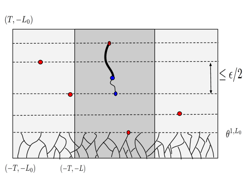
Figure 7: Schematic diagram of the proof of Lemma 4.9, when $\{\epsilon\geq 2\max_{i:\theta^{i+1,L_{0}}<T}(\theta^{i+1,L_{0}}-\theta^{i,L_{0}})\}$. Red dots are killing points on ${\mathbb{R}}\times\{\theta^{i,L_{0}}\}$ with $x$-ccordinates in $\xi^{\theta^{i,L_{0}}}(\theta^{i-1,L_{0}})$. Blue points are the starting points of the (wide) path $\pi$ (with age $\geq\epsilon$) and its extension $p$ (narrow path and its continuation $\pi$).

Lemma 4.9.

On the event $\{\epsilon\geq 2\max_{i:\theta^{i+1,L_{0}}<T}(\theta^{i+1,L_{0}}-\theta^{i,L_{0}})\}$, any path in ${\cal A}^{T,L,\epsilon}$ must be killed at some $\theta^{j,L_{0}}\in[\sigma_{\pi},T]$.

Proof.

Let us consider a path $\pi\in{\cal A}^{T,L,\epsilon}$ and and let us denote by $i$ the index such that $\sigma_{\pi}\in[\theta^{i-1,L_{0}},\theta^{i,L_{0}})$. Recall that $\pi$ is characterized by a pair $(\tilde{\pi},e_{\pi})$ where $\tilde{\pi}\in\mathcal{N}^{b}$ and $e_{\pi}$ is the killing time of $\pi$. Since the age of $\tilde{\pi}$ must be greater than $\epsilon$, on our event, there must exist $p\in\mathcal{N}^{b}$ starting at time $\theta^{i-1,L_{0}}$ and such that $p$ and $\tilde{\pi}$ coincide for $t\geq\sigma_{\tilde{\pi}}$(see Fig. 7). (We note in passing that $age(p)>0$.) Furthermore, by definition of ${\cal A}^{T,L,\epsilon}$, the path $p$ (and thus $\tilde{\pi}$) must remain in the space interval $[-L,L]$ during the time interval $[\theta^{i-1,L_{0}},\theta^{i,L_{0}}]$. By definition of $\theta^{i,L_{0}}$, it follows that $p$ (and thus $\tilde{\pi}$) must survive on $[\sigma_{\pi},\theta^{i,L_{0}})$. Using a simple induction on $j\geq i$, one can then generalize the previous reasoning to show that if $\pi$ survives up to and including $\theta^{j,L_{0}}$, it must survive up to but not including $\theta^{j+1,L_{0}}$. This implies the claim made earlier, i.e., that if $\pi$ is killed inside $(-T,T)$, $\pi$ must be killed at some $\theta^{j,L_{0}}$.

∎

Next, let us define $\theta^{i,L_{0}}_{\beta}$ analogously to $\theta^{i,L_{0}}$, i.e.,

$$\theta^{0,L_{0}}_{\beta} = -[Te^{2\beta}],$$

$$\forall i\geq 1,\ \ \theta^{i,L_{0}}_{\beta} = \inf\{t>\theta^{i-1,L_{0}}_{\beta}\ :\ \exists x\in\xi^{\theta_{\beta}^{i-1,L_{0}}}_{\beta}(t)\cap[-L_{0}e^{\beta},L_{0}e^{\beta}]\ \mbox{s.t.}\ (x,t)\ \mbox{is a killing point}\}.$$

First, by the strong Markov property and translation invariance $\{\theta^{i+1,L_{0}}-\theta^{i,L_{0}}\}$ (resp., $\{\theta^{i+1,L_{0}}_{\beta}-\theta^{i,L_{0}}_{\beta}\}$) is a sequence of i.i.d. random variables distributed like $\theta^{L_{0}}$ (resp, $\theta_{\beta}^{L_{0}}$) in (4.34). A straightforward extension of Proposition 4.4 then directly yields the following result.

Lemma 4.10.

Let us consider the set of paths $\pi\in\mathcal{N}^{b}$ (net with no killing) such that there exists $i\in{\mathbb{N}}$ so that $\sigma_{\pi}=\theta^{i,L_{0}}\in[-T,T],age(\pi)>0$ and $\max_{t\in[-T,T]}|\pi(t)|<L_{0}/2$. Under our coupling (4.35), there is a subsequence $\{{\tilde{\beta}}\}$ such that the following properties hold a.s..

1. For every $i$, $e^{-2{\tilde{\beta}}}\theta_{\tilde{\beta}}^{i,L_{0}}$ converges to $\theta^{i,L_{0}}$ a.s..

2. For every $\pi$ in the set, there exists a discrete sequence $\{\pi_{\tilde{\beta}}\}\in{\cal U}^{\tilde{\beta}}$ such that (i) $d(\pi,S_{\tilde{\beta}}(\pi_{\tilde{\beta}}))\rightarrow 0$ uniformly in $\pi$, and (ii) for ${\tilde{\beta}}$ large enough (uniformly in $\pi$),

   $$\pi\ \mbox{is killed at some $\theta^{j,L_{0}}<T$}\ \Longleftrightarrow\ \pi_{\tilde{\beta}}\ \mbox{is killed at $\theta_{\tilde{\beta}}^{j,L_{0}}$}.$$

Finally, we will need the following easy lemma.

Lemma 4.11.

Let $\{X_{\beta}\}$ be a sequence of random variables valued in ${\mathbb{R}}$. $X_{\beta}$ converges to $0$ in probability if and only for every subsequence $\{{\tilde{\beta}}\}$ and for every $\gamma>0$, one can extract a further subsequence ${\tilde{\tilde{\beta}}}$ such that ${\mathbb{P}}(\limsup_{{\tilde{\tilde{\beta}}}\uparrow\infty}|X_{\tilde{\tilde{\beta}}}|=0)\geq 1-\gamma$.

Proof.

It is well known that $X_{\beta}$ converges to $0$ in probability if and only if every subsequence has a further subsequence converging to $0$ a.s.. The lemma then follows easily. ∎

Proof of Proposition 4.6. In the following, we take $L_{0}>2L$ and we consider $\{{\tilde{\beta}}\}$ to be an arbitrary subsequence of $\{\beta\}$. By Lemma 4.10, we can extract a further subsequence $\{{\tilde{\tilde{\beta}}}\}$ – depending on $L_{0}$ – such that the relations between the discrete and continuum levels listed in this lemma hold. We will now show that

$${\mathbb{P}}(\limsup_{{\tilde{\tilde{\beta}}}\uparrow\infty}\ \max_{{\cal A}^{T,L,\epsilon}}\min_{S_{\tilde{\tilde{\beta}}}({\cal U}^{b_{{\tilde{\tilde{\beta}}}},k_{{\tilde{\tilde{\beta}}}}})}d(\pi,\pi_{\tilde{\tilde{\beta}}})\ =\ 0)\ \geq\ 1-{\mathbb{P}}(\{\epsilon\geq 2\max_{i:\theta^{i+1,L_{0}}\leq T}(\theta^{i+1,L_{0}}-\theta^{i,L_{0}})\}).$$ (4.56)

Since $L_{0}$ is arbitrarily large, our proposition follows by applying Proposition 4.5 and Lemma 4.11.

In order to show (4.56), it is sufficient to prove that for every realization of the event

$$\{\epsilon\geq 2\max_{i:\theta^{i+1,L_{0}}\leq T}(\theta^{i+1,L_{0}}-\theta^{i,L_{0}})\},$$

we must have

$$\limsup_{{\tilde{\tilde{\beta}}}\uparrow\infty}\max_{{\cal A}^{T,L,\epsilon}}\min_{S_{\tilde{\tilde{\beta}}}({\cal U}^{b_{{\tilde{\tilde{\beta}}}},k_{{\tilde{\tilde{\beta}}}}})}d(\pi,\pi_{\tilde{\tilde{\beta}}})\ =\ 0.$$

Let $\pi\in{\cal A}^{T,L,\epsilon}$ and let $i$ be such that $\sigma_{\pi}\in[\theta^{i,L_{0}},\theta^{i+1,L_{0}})$. Reasoning along the same lines as Lemma 4.9, conditional on our event, we can find a path $\pi^{\prime}\in\mathcal{N}^{b,k}$ such that (1) $\pi^{\prime}$ starts at time $\theta^{i,L_{0}}$ and $age(\pi^{\prime})>0$, (2) $\pi$ and $\pi^{\prime}$ coincide after time $\sigma_{\pi}$, and (3) $|\pi^{\prime}|<L$ on $[\theta^{i,L_{0}},\theta^{i+1,L_{0}})$ – see again Fig. 7. Since $L_{0}>2L$, the path $\pi^{\prime}$ belongs to the set of paths (at the continuum level) defined in Lemma 4.10. By definition of $\{{\tilde{\tilde{\beta}}}\}$, $\pi^{\prime}$ can be approximated (after rescaling) by a sequence $\{\pi_{\tilde{\tilde{\beta}}}^{\prime}\}$ with the properties listed in the second item of this lemma. In order to approximate $\pi$, we truncate the path $\pi_{\tilde{\tilde{\beta}}}^{\prime}$, only considering the section of $\pi_{\tilde{\tilde{\beta}}}^{\prime}$ after some time $t_{\tilde{\tilde{\beta}}}$ such that $e^{-2{\tilde{\tilde{\beta}}}}t_{\tilde{\tilde{\beta}}}\rightarrow\sigma_{\pi}$. This defines a new sequence of paths $\{\pi_{\tilde{\tilde{\beta}}}\}$ approximating the path $\pi$ and such that

$$\mbox{$\pi$ is killed at $\theta^{j,L_{0}}<T$}\Longleftrightarrow\mbox{$\pi_{\beta}$ is killed at the discrete analog $\theta^{j,L_{0}}_{\tilde{\tilde{\beta}}}$.}$$

Since any path in ${\cal A}^{T,L,\epsilon}$ must be killed at some $\theta^{j,L_{0}}\in[\sigma_{\pi},T]$ (by Lemma 4.9), and since $\{e^{-2{\tilde{\tilde{\beta}}}}\theta^{i,L_{0}}_{\tilde{\tilde{\beta}}}\}_{i}\rightarrow\theta^{i,L_{0}}$ a.s., (4.56) follows. The ends the proof of the proposition.

4.5 Step 5 : Conclusion

In this section, we prove (4.54), i.e., that any continuous path in the killed Brownian net can be uniformly approximated by a discrete killed path. In the following, we work under the coupling discussed in Lemma 4.10. We decompose the set $\mathcal{N}^{b,k}$ into three sets: (1) the set of paths killed before $-T$ or after $+T$, (2) the set of paths starting and killed on $[-T,T]$– denoted by ${\cal A}^{T}$ in the previous section – and (3) the set of paths killed on $[-T,T]$ but starting before time $-T$. In the following, we will show that when $T$ goes to $\infty$, each path in any of those subsets is well approximated by a well-chosen discrete path.

Part 1. We first consider the set of paths in $\mathcal{N}^{b,k}$ killed before time $-T$ or after $+T$.

First, let us take a path $\pi$ killed after time $T$. Any such path can be represented by a pair $(\tilde{\pi},e_{\tilde{\pi}})$, with $\tilde{\pi}$ in the Brownian net (with no killing) and $e_{\pi}$ its killing time. By convergence of the discrete net to its continuum analog, we can find $\tilde{\pi}_{\beta}$ in the discrete net approximating $\tilde{\pi}$ (after rescaling). The definition of our topology (see Section 2.1) immediately implies that $\tilde{\pi}_{\beta}$ is also a good approximation of the killed path $\pi$, provided that $T$ is large enough – intuitively, any killing point above ${\mathbb{R}}\times\{T\}$ is close to $\infty$ in our compactification of ${\mathbb{R}}^{2}$.

Analogously, since any point below the horizontal line ${\mathbb{R}}\times\{-T\}$ is close to $-\infty$, a path killed before time $-T$ is well approximated by any (properly rescaled) discrete path killed before time $-T$.

Part 2. We now approximate the set of paths starting and killed in the interval $[-T,T]$. As usual, $\square_{L,T}$ will refer to the box $[-L,L]\times[-T,T]$. We will also make use of the following notation. First, we write ${\cal A}^{T,L}$ for the set of the paths killed during the time interval $[-T,T]$, and staying in the space interval $[-L,L]$ during this time period – with no restriction on the age of the path. Note that ${\cal A}^{T,L}\equiv{\cal A}^{T,L,0}$, where ${\cal A}^{T,L,\epsilon}$ was defined in the previous section. Next, define

$${\cal B}^{T,L} : \mbox{ paths $\pi\in{\cal A}^{T}$ with $|\pi(\sigma_{\pi})|<L$},$$

$$\bar{\cal B}^{T,L} : \mbox{ paths $\pi\in{\cal A}^{T}$ with $|\pi(\sigma_{\pi})|\geq L$},$$

$$\bar{\cal A}^{T,L} : \pi\in{\cal A}^{T} |\pi|\geq L \square_{L,T}$$ paths with on .

Finally, the same notation, but with an extra $\beta$ subscript, will refer to the analogous quantities for the rescaled set $S_{\beta}({\cal U}^{b_{\beta},k_{\beta}})$. Next,

$${\mathbb{P}}\left(\max_{{\cal A}^{T}}\min_{S_{\beta}({\cal U}^{b_{\beta},k_{\beta}})}d(\pi,\pi_{\beta})\ >\ \gamma\right) \leq {\mathbb{P}}\left(\max_{{\cal B}^{T,3L}}\min_{S_{\beta}({\cal U}^{b_{\beta},k_{\beta}})}d(\pi,\pi_{\beta})\ >\ \frac{\gamma}{2}\right),+{\mathbb{P}}\left(\max_{\bar{\cal B}^{T,3L}}\min_{S_{\beta}({\cal U}^{b_{\beta},k_{\beta}})}d(\pi,\pi_{\beta})\ >\ \frac{\gamma}{2}\right),$$ (4.57)

$$\leq {\mathbb{P}}\left(\max_{{\cal A}^{T,4L}}\min_{S_{\beta}({\cal U}^{b_{\beta},k_{\beta}})}d(\pi,\pi_{\beta})\ >\ \frac{\gamma}{2}\right)+{\mathbb{P}}\left(\max_{\bar{\cal A}^{T,2L}}\min_{S_{\beta}({\cal U}^{b_{\beta},k_{\beta}})}d(\pi,\pi_{\beta})\ >\ \frac{\gamma}{2}\right)$$

$$+2\left(1-{\mathbb{P}}({\cal B}^{T,3L}\subset{\cal A}^{T,4L},\ \ \bar{\cal B}^{T,3L}\subset\bar{\cal A}^{T,2L})\right).$$

Part 2 follows by taking successively $L$ and then $T$ to $\infty$ and using the three following lemmas.

Lemma 4.12.

$$\forall L,T,\ \ \ \lim_{\beta\uparrow\infty}\max_{{\cal A}^{T,L}}\min_{S_{\beta}({\cal U}^{b_{\beta},k_{\beta}})}d(\pi,\pi_{\beta})=0\ \mbox{in law.}$$

Proof.

In the previous section, we showed this result for ${\cal A}^{T,L,\epsilon}$ with $\epsilon>0$. We now would like to extend this result to the case $\epsilon=0$.

Case 1. $\pi$ is killed after time $\sigma_{\pi}+\epsilon$. Let us consider $\bar{\pi}$, the section of the path after $\sigma_{\pi}+\epsilon$. In particular, the age of $\bar{\pi}$ is equal to $\epsilon$ and by Proposition 4.6, we can approximate the path $\bar{\pi}$ by a discrete path $\bar{\pi}_{\beta}\in S_{\beta}({\cal U}^{b_{\beta},k_{\beta}})$. The two main contributions to the distance between $\bar{\pi}_{\beta}$ and $\pi$ are (1) the difference in starting time – equal approximatively to $\epsilon$ and (2) the variation of $\pi$ on $[\sigma_{\pi},\sigma_{\pi}+\epsilon]$. As $\epsilon\downarrow 0$, the first term vanishes. Since the compactness of $\mathcal{N}^{b,k}$ implies equicontinuity of the net paths in the rectangle $[-L,L]\times[-T,T]$ (by Arzela-Ascoli), the second term also vanishes (uniformly in $\pi$).

Case 2. $\pi$ is killed in $[\sigma_{\pi},\sigma_{\pi}+\epsilon]$. Let us consider the quantity

$$\max_{z\in\square_{L,T}}\max_{z^{\prime}\in S_{\beta}({\cal M}^{k_{\beta}}_{\beta})}\ \ \rho(z,z^{\prime}),$$

the maximum distance between a point in the box $\square_{L,T}$ from the set of rescaled discrete killing points. By a standard Borel-Cantelli argument, this quantity a.s. goes to $0$. Thus, we can always find a sequence of discrete killing points $\{z_{\beta}\}$ converging (after rescaling) to the starting point of $\pi$ as $\beta$ goes to $\infty$. Considering the path consisting of the single point $z_{\beta}$ (starting and ending at the same point), this path is a good approximation of $\pi$ for $\epsilon$ small enough.

∎

Lemma 4.13.

$$\forall T>0,\ \ \lim_{L\uparrow\infty}\lim_{\beta\uparrow\infty}\ \ \ \max_{\bar{\cal A}^{T,L}}\min_{S_{\beta}({\cal U}^{b_{\beta},k_{\beta}})}d(\pi,\pi_{\beta})\ =\ 0,\ \ \ \ \mbox{in law}.$$

Proof.

Here we consider the paths $\pi\in\bar{\cal A}^{T,L}$ with $\sigma_{\pi}\geq-T$. The case $\sigma_{\pi}<-T$ can easily be deduced from the previous case by approximating the section of the path after time $-T$.

Let $\gamma>0$ be an arbitrarily small number such that $T/\gamma\in{\mathbb{N}}$. We claim that for $\beta$ large enough, for every $i,j\in{\mathbb{Z}}$ such that $i\leq j$ and $|i\gamma|,|j\gamma|\leq T$, there exists a.s. a path $\pi_{\beta}$ in $\bar{\cal A}^{T,L}_{\beta}$ with $\pi_{\beta}>L$ starting from the interval $[i\gamma,(i+1)\gamma)$ and killed in the interval $[j\gamma,(j+1)\gamma)$. Before proving this, we first show how this implies our lemma. By definition of the distance between paths, for every $\pi,\pi_{\beta}$ such that $\pi,\pi_{\beta}>L$ for all $t\in[-T,T]$, we must have

$$d(\pi,\pi_{\beta}) \leq |\psi(\sigma_{\pi})-\psi(\sigma_{\pi_{\beta}})|+|\psi(e_{\pi})-\psi(e_{\pi_{\beta}})|+(1-\tanh(L)).$$

where $\psi=\tanh(t)$, as in Section 2.1. (Note that the third term corresponds to the fact that two points with the same time coordinate and space coordinate $>L$ are close to each other in our topology when $L$ is large.) For any path $\pi\in\bar{\cal A}^{T,L}$, let $i,j$ be such that $\sigma_{\pi}\in[i\gamma,(i+1)\gamma)$ and $e_{\pi}\in[j\gamma,(j+1)\gamma).$ Finally, let us consider any path $\pi_{\beta}>L$ in $\bar{\cal A}^{T,L}_{\beta}$ with its starting and ending times belonging to the same time intervals (which exists by the claim made earlier). By the previous inequality, we must have

$$d(\pi,\pi_{\beta}) \leq 2\gamma+(1-\tanh(L)).$$

By symmetry, the same discrete approximation can be obtained for a path $\pi\in\bar{\cal A}^{T,L}$ with $\pi<-L$. Hence, we get that for $\beta$ large enough

$$\max_{\bar{\cal A}^{T,L}}\min_{S_{\beta}({\cal U}^{b_{\beta},k_{\beta}})}d(\pi,\pi_{\beta})\leq 2\gamma+(1-\tanh(L)),$$

implying that

$$\lim_{L\uparrow\infty}\lim_{\beta\uparrow\infty}\ \ \ {\mathbb{P}}(\max_{\bar{\cal A}^{T,L}}\min_{S_{\beta}({\cal U}^{b_{\beta},k_{\beta}})}d(\pi,\pi_{\beta})\ \leq\ 3\gamma)=1.$$

Since this is true for every $\gamma>0$, the result follows.

It remains to show the claim made earlier. In order to prove this, for every $K\in{\mathbb{N}}\setminus\{0\}$, let us consider the box $((2K-1)L,(2K+1)L)\times[-T,T],$ and the rescaled left-most path in $\bar{\cal A}^{T,L}_{\beta}$ starting at the point $(2K\cdot L,(i\gamma)_{\beta})$, where $(i\gamma)_{\beta}$ denotes the point in ${\mathbb{Z}}e^{-2\beta}$ defined as $([i\gamma e^{2\beta}]+1)e^{-2\beta}$. This walk is distributed like a drifted rescaled random walk, killed at each microscopic step with a probability equal to $k_{\beta}$. For $\beta$ large enough (e.g., such that $e^{-2\beta}<\gamma/2$) there exists a time in the lattice ${\mathbb{Z}}e^{-2\beta}$ and belonging to the interval $[j\gamma,(j+1)\gamma)$. For such $\beta$, there exists a strictly positive probability for the event $F_{\beta}^{K,\gamma,i,j}$ to occur, where $F_{\beta}^{K,\gamma,i,j}$ is defined as the event that our walk stays in the box $((2K-1)L,(2K+1)L)\times[-T,T]$ and is killed in the time interval $[j\gamma,(j+1)\gamma]$. By independence of the elements of the sequence $\{F_{\beta}^{K,\gamma,i,j}\}_{K\geq 1}$, there must exist a.s. a $K$ such that the event $F_{\beta}^{K,\gamma,i,j}$ occurs. Since for $\beta$ large enough, our walk obviously starts from the interval $[i\gamma,(i+1)\gamma)$, this implies the claim made earlier and ends the proof of our lemma.

∎

Lemma 4.14.

$$\forall T>0,\ \lim_{L\uparrow\infty}{\mathbb{P}}\left({\cal B}^{T,3L}\subset{\cal A}^{T,4L},\ \ \ \bar{\cal B}^{T,3L}\subset\bar{\cal A}^{T,2L}\right)\ =\ 1.$$

Proof.

Let us consider $l$, the left-most path in the (non-killed) Brownian net starting from $(-T,2.5L)$, and $r$ the right-most path starting from $(-T,3.5L)$. We also define $\tilde{l},\tilde{r}$ the left-most and right-most path starting respectively from $(-T,-3.5L)$ and $(-T,-2.5L)$. Finally, let us consider the event that

$$\min_{[-T,T]}l>2L,\max_{[-T,T]}l<3L, \min_{[-T,T]}r>3L,\ \max_{[-T,T]}r<4L\ \ \mbox{and}$$ and

$$\max_{[-T,T]}\tilde{r}<-2L,\min_{[-T,T]}\tilde{r}>-3L, \max_{[-T,T]}\tilde{l}<-3L,\ \min_{[-T,T]}\tilde{l}>-4L.$$ and

Using the fact that there is no path of the Brownian net crossing a left-most path (resp., right-most path) from the right (resp., from the left) it is easy to see that under the event above, we must have

$${\cal B}^{T,3L}\subset{\cal A}^{T,4L},\ \ \ \bar{\cal B}^{T,3L}\subset\bar{\cal A}^{T,2L}.$$

For instance, any path starting from the right of the vertical line $\{3L\}\times{\mathbb{R}}$ can not enter the box $\square_{L,2T}$ since it is blocked by the path $l$. On the other hand, any path starting in the box $\square_{L,2T}$ is unable to exit the box $\square_{L,4T}$ since it is blocked by the paths $r$ and $\tilde{l}$.

Since left-most and right-most paths starting from deterministic points are distributed like drifted Brownian motions, when $L$ goes to $\infty$ for fixed $T$, the event above is realized with probability going to $1$. This ends the proof of our lemma.

∎

Part 3. We end the proof of Theorem 1.1 by considering the set of paths starting before time $-T$ and killed on the time interval $[-T,T]$. Let $\pi$ be such a path and let us consider $\pi^{\prime}$, the section of $\pi$ after time $-T$. This path obviously belongs to ${\cal A}^{T}$ and by the previous part, it can be approximated by a sequence of discrete paths $\{\pi_{\beta}^{\prime}\}$. The main contributions to the distance between $\pi$ and $\pi_{\beta}^{\prime}$ are (1) the difference in their starting time and (2) the variation of $\pi$ on $[\sigma_{\pi},-T]$. However, for $T$ large enough, any point below the line ${\mathbb{R}}\times\{-T\}$ is close to $-\infty$. Thus, as $T$ goes to $\infty$, the difference vanishes.

5 List of Main Symbols

$$\begin{array}[]{ccc}{\mathbb{Z}}_{even}^{2}&\mbox{Even square lattice }&\mbox{Section}\ \ref{intro}\\ \beta&\mbox{Scaling parameter}&\mbox{Section}\ \ref{intro}\\ {\cal U}^{b_{\beta},k_{\beta}}&\mbox{Banching-Coalescing-Killing system}&\mbox{Section}\ \ref{intro}\\ {\cal U}^{b_{\beta}}&\mbox{Banching-Coalescing system}&\mbox{Section}\ \ref{intro}\\ \sigma_{\pi}&\mbox{Starting time of the path $\pi$}&\mbox{Section}\ \ref{intro}\\ e_{\pi}&\mbox{Ending time of the path $\pi$}&\mbox{Section}\ \ref{intro}\\ S_{\beta}(x,t)&\mbox{Rescaling of space-time points.}&p.\ref{scal-transf}\\ d&\mbox{Distance between paths}&p.\ref{diistance}\\ d_{{\cal H}}&\mbox{Distance between compact sets of paths}&p.\ref{dh}\\ {\cal W}&\mbox{Brownian web}&p.\ref{Forward_Web}\\ (m,n)\ \mbox{points}&\mbox{Special points of the Brownian web}&p.\ref{special_points}\\ {\mathcal{N}}^{b}&\mbox{Brownian net}&p.\ref{standard-net}\\ (\mathcal{W}_{l},\mathcal{W}_{r})&\mbox{Pair of left-most and right-most Brownian webs.}&p.\ref{standard-net}\\ \sim^{in}_{z}&\mbox{Equivalence relation for paths entering a point.}&p.\ref{eq:in-out}\\ \sim^{out}_{z}&\mbox{Equivalence relation for paths exiting a point.}&p.\ref{eq:in-out}\\ (p,p),(0,pp)\cdots&\mbox{Special points of the Brownian net}&p.\ref{special-force}\\ {\xi^{S}}&\mbox{Branching Coalescing (BC) point set (with no killling) starting form ${\mathbb{R}}$ at time $0$}&p.\ref{df-age}\\ {\mathcal{N}^{b,k}}&\mbox{Brownian net with killing}&p.\ref{onenet}\\ {{\cal M}^{k}}&\mbox{Set of killing points.}&p.\ref{onenet}\\ {age(x,t)}&\mbox{Age of a point}&p.\ref{age}\\ {{\cal T}^{\delta}}&\mbox{Time length measure on the $\delta$-shorteneing of the Brownian net.}&p.\ref{continuous-tl}\\ \theta^{L}&\mbox{First killing time}&p.\ref{thetaL}\\ \theta^{i,L,T}&\mbox{Sequence of killing times}&p.\ref{thetail}\\ \end{array}$$

Acknowledgments. The research of C.M.N. is supported in part by NSF grants OISE-0730136, DMS-1007524 and DMS-1007626.

References

- [A81] R. Arratia, Coalescing Brownian motions and the voter model on , Unpublished partial manuscript (circa 1981), available from rarratia@math.usc.edu.
- [CDP11] J.T. Cox, R. Durrett, E. Perkins. Voter model perturbations and reaction diffusion equations. Astérisque. 349, (2013).
- [FINR04] L.R.G. Fontes, M. Isopi, C.M. Newman, K. Ravishankar. The Brownian web: characterization and convergence. Ann. Probab. 32, (2004), 2857–2883.
- [FINR05] L.R.G. Fontes, M. Isopi, C.M. Newman, K. Ravishankar. Coarsening, nucleation, and the marked brownian web. Ann. Inst. H. Poincaré, Probab. et Stat. 42, (2006), 37-60.
- [HL75] R. Holley, T. Liggett. Ergodic theorems for weakly interacting infinite systems and the voter model. Annals of Probability. 3, (1975), 643-663.
- [KS91] I. Karatzas, E. Shreve. Brownian Motion and Stochastic Calculus, Springer-Verlag, Berlin-Heidelberg-New York, 1991.
- [K91] A.F. Karr. Point Processes and their statistical inference. (1991). 2nd ed., Probability: Pure and Applied, vol. 7, Marcel Dekker Inc., New York.
- [L04] T. Liggett. Interacting particle systems. (2004). Springer, Berlin-Heidelberg-New York.
- [MNR13] Y. Mohylevskyy, C. M. Newman, K. Ravishankar. Ergodicity and percolation for variants of one-dimensional voter models. ALEA. 10, (2013), 485–504.
- [MoDDGL99] J. Molofsky, R. Durrett, J. Dushoff, D. Griffeath, S. Levin, Local frequency dependence and global coexistence. Theor. Pop. Biol. 55, (1999), 270—282.
- [NP99] C. Neuhauser, S.W. Pacala, An explicitly spatial version of the Lotka-Volterra model with interspecific competition. Ann. Appl. Probab. 9, (2000), 1226—1259.
- [NRS10] C.M. Newman, K. Ravishankar, E. Schertzer. Marking the points of the Brownian web and applications. Ann. Inst. H. Poincaré. 46, (2010), 537—574.
- [NRS13] C.M. Newman, K. Ravishankar, E. Schertzer. Voter model perturbations in one dimension. In preparation.
- [OHLN06] H. Ohtsuki, H. C. Hauert, E. Lieberman, M.A. Nowak. A simple rule for the evolution of cooperation on graphs and social networks. Nature. 441, (2006), 502—505.
- [SSS09] E. Schertzer, R. Sun, J.M. Swart. Special points of the Brownian net. Electr. J. Prob.. 14, (2009), 805—854.
- [SSS13] E. Schertzer, R. Sun, J.M. Swart. Stochastic flows in the Brownian web and net. A.M.S. Memoirs. 227 (in press).
- [STW00] F. Soucaliuc, B. Tóth, W. Werner, Reflection and coalescence between independent one-dimensional Brownian paths, Ann. Inst. H. Poincaré, Probab. et Stat. 36, (2000), 509–545.
- [SS08] R. Sun, J.M. Swart. The Brownian net. Ann. Probab. 36, (2008), 1153–1208.
- [TW98] B. Tóth, W. Werner. The true self-repelling motion. Probab. Th. Rel. Fields 111, (1998), 375–452.