Holographic Superconducting Quantum Interference Device

Shingo Takeuchi${}^{\dagger\,\ddagger}$

$\dagger$ Shanghai Jiao Tong University, Shanghai 200240, China
$\ddagger$ The Institute for Fundamental Study “The Tah Poe Academia Institute”
Naresuan University Phitsanulok 65000, Thailand
shingo(at)nu.ac.th

We present a holographic model of the SQUID (Superconducting QUantum Interference Device) in the external magnetic field. The model of the gravitational theory considered in this paper is the Einstein-Maxwell-complex scalar model on the four-dimensional Anti-de Sitter Schwarzschild black brane geometry, where one space direction is compacted into a circle and we arrange the coefficient of the time components profile so that we can model the SQUID, where the profile plays the role of the chemical potential for the cooper pair.

1 Introduction

In recent years, we have been studying the superconductors using the potential applicability of anti-de Sitter (AdS)/conformal field theory (CFT) correspondence [1, 2, 3]. The notable examples are Refs.[4, 5, 6], Refs.[7, 8, 9] and Ref.[10] which have provided the gravity duals for the superconductors, the (non-)Fermi liquids, and the superconductor/insulator transition at zero temperature, respectively. Further the s-  , p- and d-wave superconductors have been also thoroughly investigated. Although we cannot refer to each paper for these, for example see [11] for its synthetic report.

One of the interesting topics associated with the superconductivity would be the Josephson junction [12], and now there are many developing studies of the holographic version. The first paper was Ref.[13], in which the superconductor-normal metal-superconductor (SNS) Josephson junction was studied holographically. After that, toward Ref.[13], the dimensional extension was discussed in Refs.[14, 15], and generalized to the p-wave Josephson junction as discussed in Ref.[16]. Ref.[17] provided the gravity dual for a superconductor-insulator-superconductor (SIS) Josephson junction. Ref.[18] invented the holographic Josephson junction based on the designer multigravity (namely multi-(super)gravity theories). Ref.[19] constructed a Josephson junction in the non-relativistic case with a Lifshitz geometry as the dual gravity.

The superconductors in the external magnetic field would be intriguing, and its holographic study has also been developing. The first papers are Refs.[6, 20, 21, 22], and although we cannot refer to all the papers, the papers we have particularly checked in this paper are Refs.[23, 24, 25, 26, 27] along with those four papers.

This paper will be devoted to a holographic SQUID (Superconducting QUantum Interference Device) consisting of two Josephson junctions with the external magnetic field shown in Fig.1. The significance in the holographic study of the Josephson junction and the SQUID would be the application to the case where the coupling constants become strong in a system occupied by two different parts. For instance, we take an issue with whether the two supercoductors can stick each other perfectly or not when they are put separately with some distance ($L$) in between some empty space without the mid materials. Since it is known that the free energy for such two supercoductors is a decreasing function when $L$ becomes smaller [28], they move close to each other. Here we assume that no friction occurs when these supercoductors move. However, when $L$ becomes very small, the quantum effect becomes strong. As a result, it is difficult to conclude whether two supercoductors can stick to each other perfectly or not eventually. It is very interesting if this issue relates to the issue whether evaporating black holes vanish or remain eventually by regarding the empty space as the evaporating black holes and two superconductor parts as the space of the outside of the black holes. In such an issue, the strongly coupled analysis is very important, and the skill developed in the holographic Josephson junctions and the SQUID like ones in this paper could be a big help.

Lastly, we give a comment on the same type of the holographic SQUID in Ref.[29]. Originally, there are two supercurrents in the SQUID as represented as $J_{L}$ and $J_{R}$ in the left and the right sides of the SQUID in Fig.1. On the other hand, in Ref.[29], only one supercurrent is considered. Despite this, they measure the phase differences in the left and the right Josephson junctions, $\Delta\theta_{L}$ and $\Delta\theta_{R}$, where $\Delta\theta_{L}$ and $\Delta\theta_{R}$ are shown in Fig.1. However, their way to measure the phase differences from one current is not clear. This has motivated us to carry out this paper. In this paper, another way for the holograhic SQUID in the magnetic field is proposed, and we can confirm that we can obtain the result consistent with the original SQUID in the external magnetic field and the result in Ref.[29].

Regarding the organization of this paper;  Section.2 is devoted to brief review of the SQUID we will consider in this paper: the points in our holographic way to model the SQUID, which are how to take in the magnetic flux and how to take in the specific behavior of the supercurrent and the conclusion of this paper. In section.3, we give our gravity model and the equations of motion. Further, we mention about the ansatz. In section.4, we show the results of our analysis in our holographic SQUID. In Appendix A, we explain the validity of a condition used in Section.2. In Appendix B, we list the numerical results in section.4 explicitly.

2 Brief review of SQUID, our holographic way to model it and conclusion

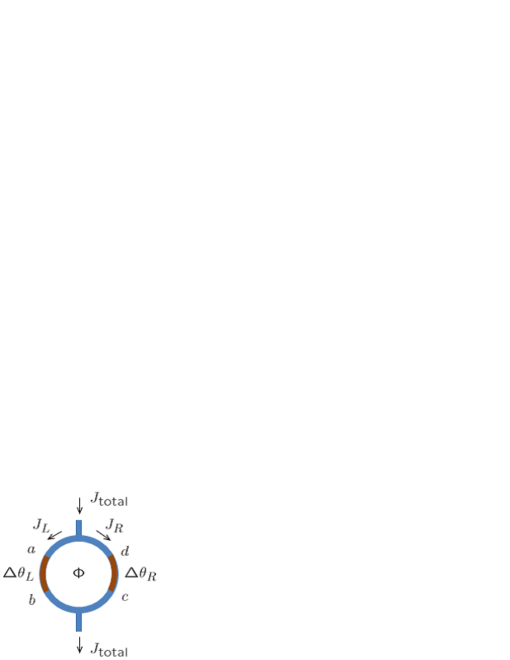
Figure 1: The SQUID blueconsidered in this paper. For the meaning of each character and the figure, see the body text.

We devote this section to a brief review of the SQUID we consider in this paper and the points in our holographic way to model it.

2.1 Brief review of SQUID in this paper

The SQUID we consider in this paper is given by connecting two Josephson junctions in a circle and attaching two branches for the inflowing and outflowing supercurrents $J_{\rm total}$. We show it schematically in Fig.1.

In Fig.1, $\Phi$ represents the magnetic flux, and the blue and the brown parts represent the superconductor and the normal metal parts, respectively. Then the wave functions in the superconductor parts are condensed in a phase. As a result, the phase differences arise in the intervals of the normal metal parts $a-b$ and $c-d$, and $\Delta\theta_{L}$ and $\Delta\theta_{R}$ represent such phase differences in the intervals of the normal metal parts $a-b$ and $c-d$. As a result, the supercurrent is induced by the Josephson effect [12], and $J_{L}$ and $J_{R}$ represent such supercurrents flowing in the left and the right sides of the circuit of SQUID. These are known to be written with the sine function as

$$J_{L}=I_{cL}\sin\Delta\tilde{\theta}_{L}\quad\textrm{and}\quad J_{R}=I_{cR}\sin\Delta\tilde{\theta}_{R},$$ (2.1)

where $I_{cL}$ and $I_{cR}$ are constants meaning the maximal supercurrent and $\Delta\tilde{\theta}_{L}$ and $\Delta\tilde{\theta}_{R}$ presents the gauge invariant phase differences defined as $\displaystyle\Delta\tilde{\theta}_{L}\equiv-\frac{e^{*}}{\hbar}\int_{a}^{b}{\bf A}\cdot{\rm d{\bf l}}+\Delta\theta_{L}$ and $\displaystyle\Delta\tilde{\theta}_{R}\equiv-\frac{e^{*}}{\hbar}\int_{c}^{d}{\bf A}\cdot{\rm d{\bf l}}+\Delta\theta_{R}$, and we obtain this sine relation later in Fig.7. Here $e^{*}$ represents the electric charge of a cooper pair forming the supercurrents, $d\bf l$ represents the line elements along the circuit of the SQUID and ${\bf A}$ represents the gauge field on the circuit, and ‘$a$’, ‘$b$’, ‘$c$’, ‘$d$’ are the locations on the circuit in Fig.1. Consequently, the total amount of the inflowing supercurrent $J_{\rm total}$ can be written as

$$J_{\rm total} = J_{L}-J_{R}$$ (2.2)

$$= 2J_{c}\cos\left(\frac{\Delta\tilde{\theta}_{L}+\Delta\tilde{\theta}_{R}}{2}\right)\sin\left(\frac{\Delta\tilde{\theta}_{L}-\Delta\tilde{\theta}_{R}}{2}\right),$$

where we have assumed that $J_{cL}=J_{cR}\equiv J_{c}$ for simplicity and assigned the minus sign to $J_{R}$ taking into account the fact that we measure the phases in an anticlockwise direction in the circuit of Fig.1.

Here the contour integral of the infinitesimal variation of the phase $\nabla\theta$ along the circuit of the SQUID should be given by integral multiplication of $2\pi$ as $\displaystyle 2\pi n=\oint\nabla\theta\cdot{\rm d{\bf l}}$, where $n$ means some integer number and $\nabla\theta$ is known to be given in the condensed matter physics as $\nabla\theta=(m^{*}{\bf v}_{s}+e^{*}{\bf A})/\hbar$ (${\bf v}_{s}$ and $m^{*}$ are the velocity and the mass of the cooper pairs, while $e^{*}$ has been defined above). Evaluating the right hand of it, it turns out that this contour integral can be written as

$$2\pi n=2\pi\frac{\Phi}{\Phi_{0}}+\Delta\tilde{\theta}_{L}+\Delta\tilde{\theta}_{R},$$ (2.3)

where $\Phi_{0}\equiv h/e^{*}$ and $\Phi$ means the magnetic flux penetrating the circuit of the SQUID, $\displaystyle\Phi=\int(\nabla\times{\bf A})\cdot d{\bf S}$, where $d\bf S$ means the area element. Here to derive the above relation, ${\bf v}_{s}$ is taken to zero (${\bf v}_{s}=0$) in the superconductor parts of the circuit of the SQUID by assuming that the path of the integration goes through the center of the section of the circuit. We give a description to validate this ${\bf v}_{s}=0$ in Appendix A.

Then using the relation (2.3), eq.(2.2) can be rewritten as

$$J_{\rm total} = J_{\rm max}(\Phi)\sin\left(\Delta\tilde{\theta}_{L}+\pi\frac{\Phi}{\Phi_{0}}\right)\quad\textrm{with}\quad J_{\rm max}(\Phi)\equiv 2J_{c}\cos\left(\pi\frac{\Phi}{\Phi_{0}}\right),$$ (2.4)

where the above has been obtained with $n=0$ in eq.(2.3). The behavior of $J_{\rm max}(\Phi)$ against the magnetic flux $\Phi$ is one of the specific behavior of SQUID, and we will aim to reproduce it in our holographic SQUID, and the result is given in Fig.8.

2.2 Our holographic SQUID

Now that we have reviewed the condensed matter physics side, we will turn to the points in our way to model the holographic SQUID, which are how to involve the magnetic flux and the flow of the supercurrent. Explicit descriptions of our model are presented after this section.

The background geometry in this paper will be the four-dimensional Anti-de Sitter Schwarzschild black brane geometry. Then the boundary space is given by 1+2 dimensional space. We compactify a direction of either of the two space directions into a $S^{1}$ circle, which means that the boundary space in this paper is given as the surface of the cylinder. We illustrate the boundary space in Fig.2 on which the dual field theory lives.

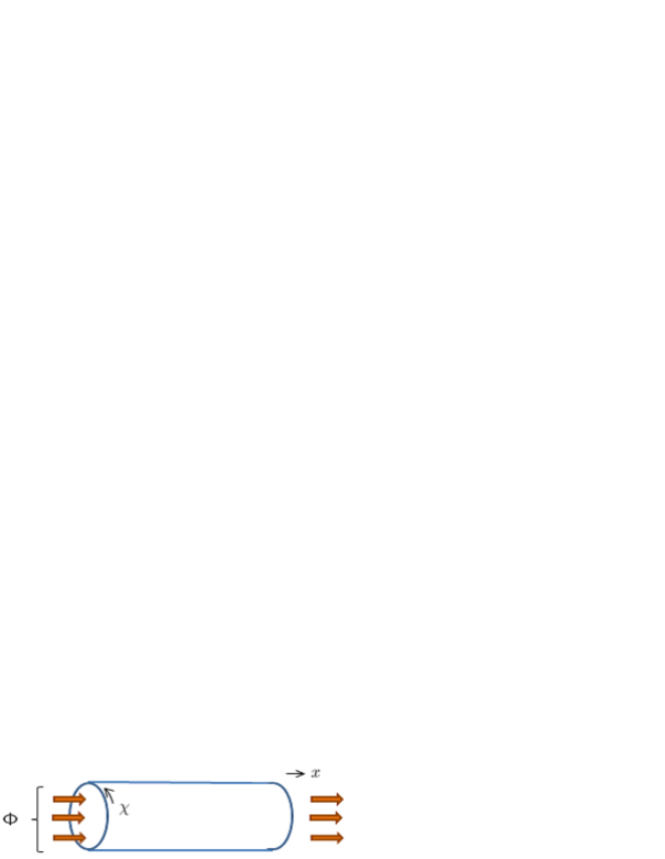
Figure 2: This figure illustrates the boundary space on which the dual field theory lives. Here our boundary space is given not as the cylinder including its interior, but as the surface of the cylinder. We refer to the circled direction as $\chi$-direction. Then we put our holographic SQUID on $\chi$-direction in the form of the loop. $\Phi$ represents the magnetic flux running in the interior of the cylinder, which itself is fictitious (due to the absence of the interior space) but finally we can involve the effect of the magnetic flux $\Phi$ by the rewriting of the surface integral of the magnetic field to the contour integral of the gauge field [26, 27] as mentioned in the body text.

We realize our holographic SQUID on the $S^{1}$ circled space in the form that it winds around the $S^{1}$ circle. The SQUID is composed of two Josephson junctions as can be seen in Fig.1. Then to model such double holographic Josephson junctions, we arrange the time component of the gauge field appropriately by exploiting its $\chi$ dependence as in eq.(3.5) as well as Ref.[13], where the coefficients appearing in the expansion around the horizon are known to have the roles of the density (charge) and the chemical potential. (For example, see Ref.[31]). In what follows, we refer the circled direction as $\chi$-direction. For more concrete description of our model, see Section.3.

Here we mention one of the issues in our holographic model, which is how to involve the magnetic flux. First, the space where the dual field theory lives does not include the interior space of the cylinder. Hence, the magnetic flux penetrating the circuit of the SQUID cannot exist in the dual field theory. However, temporarily considering the interior space of the cylinder in the space of the dual field theory, let us assume that the magnetic flux $\Phi$ given by the area integral $\displaystyle\Phi=\int d{\bf S}\cdot{\bf B}$ exists. Then considering the external gauge field $a_{\chi}(\chi)$ in the space of the dual field theory on the surface of the cylinder, $\Phi$ can be rewritten to the line integral using the Stokes’s theorem as $\displaystyle\Phi=\oint_{\chi}d\chi\,a_{\chi}(\chi)$. Here we write the coefficient of the $\chi$ component of the gauge field when it is expanded in the vicinity of the boundary in the bulk gravity as $\nu(\chi)$. Then we can link the magnetic flux $\Phi$ that we have spuriously assumed above to the external gauge field $\nu(\chi)$ actually existing in our model as

$$\Phi=\oint_{\chi}d\chi\,\nu(\chi).$$ (2.5)

Hence, in the conclusion, despite the fact we cannot have the magnetic flux itself, we can fictitiously involve the effect of the magnetic flux. (This way has been performed in refs.[26, 27].)

We have another issue, which is the effect of the branches appearing in Fig.1. First, since there is no branch in our holographic model of the SQUID, our holographic SQUID is just a loop consisting of two Josephson junctions. If there are the branches, the supercurrent inflows from the above, separates into two flows, and finally outflows to the below. On the other hand, if it were not for the branches, the circuit of the SQUID would become a simple loop and the supercurrent simply circulates in the circuit of the SQUID.

If we try to involve the effect of the branches, we have to consider the boundary condition such that all the fields in three sectors, the left, the right and the branch parts, continuously connect to each other at the joint parts between the circuit and the branches. However, such a boundary condition is very difficult to treat. Hence in this paper, considering that there is no continuity condition at the joint parts in the circuit of the SQUID in Fig.1, the SQUID we consider is the one without the branches and separated into the left and the right parts as in the left figure of Fig.3, where the meaning of the separation is mentioned in what follows.

First we mention the reason for having no continuity condition. Since the supercurrent suddenly splits at the top aof the joint part and merges at the bottom joint part, the amount of the supercurrent varies rapidly at the joint parts, which is mostly discontinuous. Therefore, we can consider that the fields at the joint parts are discontinuous. Then we mention about separating into the left and the right parts in Fig.3. Since there is no continuity condition as mentioned above, we can consider that there is no interference between the two Josephson junctions. Therefore, we perform the analysis not for the two Josephson junctions interfering with each other but for each side of the Josephson junction separately.

After this, we reference how to obtain the result of the SQUID from two such independent Josephson junctions. First, we assume that we have obtained the results for one Josephson junction with no interaction with the other Josephson junction. Actually, the result for one Josephson junction is presented in Fig.7, and the numerical data on which Fig.7 is based is presented in Table.1 of Appendix B, Then we choose the value of the supercurrents from Table.1 and simply treat these as the amount of the supercurrent flowing in the each side. Accompanying this, the phase differences in each Josephson junction are chosen. Then from the value of the supercurrents and the phase differences we have set here, according to eq.(2.3), the magnetic flux $\Phi$ can be fixed. Then now that we have the information of the supercurrents in each side and the magnetic flux $\Phi$, we can obtain the values of $J_{\rm max}(\Phi)$ in eq.(2.4), and finally obtain the results of the SQUID, which is Fig.3.

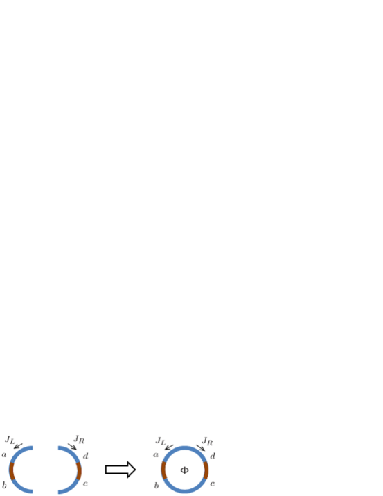
Figure 3: This figure illustrates that we simply consider the SQUID as the one except for the branches, and separate it into the left and the right parts. Then performing the analysis in each side one at a time separately, we finally consider the result of a SQUID by simply joining the results of these two analysis.

3 Holographic setup to model SQUID

In this paper, we consider the following action

$$S=\int d^{4}x\;\sqrt{-g}\left[R+\frac{6}{L^{2}}-\frac{1}{4}F_{\mu\nu}F^{\mu\nu}-|D\psi|^{2}-m^{2}|\psi|^{2}\right],$$ (3.1)

where $\mu,\nu=1,\cdots,4$, $A_{\mu}$ is U(1) gauge field and $F_{\mu\nu}=\partial_{\mu}A_{\nu}-\partial_{\nu}A_{\mu}$. Further, $D_{\mu}\equiv\nabla-iqA_{\mu}$ and $m^{2}=-2$. We take the probe approximation in our analysis, which can be obtained by rescaling $\psi=\tilde{\psi}/q$, $A=\tilde{A}/q$ and taking $q\rightarrow\infty$ with fixing $\tilde{\psi}$ and $\tilde{A}$.

One of the solutions in model (3.1) is the four-dimensional Anti-de Sitter Schwarzschild black brane geometry,

$${\color[rgb]{0,0,0}ds^{2}=\frac{1}{z^{2}}\left(-f(z)dt^{2}+\frac{1}{f(z)}dz^{2}\right)+r^{2}(dx^{2}+d\chi^{2}),}$$ (3.2)

where $f(r){\color[rgb]{0,0,0}=}1-z^{3}/z_{0}^{3}$ and $z_{0}$ mean the location of the horizon. $\chi$-direction is $S^{1}$ compactified with the periodicity $-\pi R\leq\chi\leq\pi R$ with $\pi R=7$  (For convenience in our actual analysis, we have taken this a number). Here the Hawking temperature is given as $T=3/(4\pi L^{2}z_{0})$. We fix the AdS radius $L$ and $r_{0}$ as $L=1$ and $z_{0}=1$, respectively. As a result, the temperature in this paper is given as $T=3/(4\pi)$.

Here let us give a comment on another geometry. The soliton geometry [30] is also one of solutions in the model (3.1). However, in the case of the soliton geometry, due to the vacuum current and the difference in the fluxoid number [26], the analysis will be very involved. Therefore in this paper, we fix the background geometry to the black brane geometry, and the boundary space is given as the surface of a cylinder. Here it is known [10] that the black brane geometry (3.2) is energetically favorable towards the soliton geometry provided that $T>1/(2\pi R)$ with $R$ taken as $R=7/\pi$ in this paper.

As an ansatz, we think that all the fields can be written as follows:

$$\tilde{\psi}(z,\chi) = \overline{\psi}(z,\chi)e^{i\varphi(z,\chi)},$$ (3.3)

$$\tilde{A}(z,\chi) = A_{t}(z,\chi)dt+A_{z}(z,\chi)dz+A_{\chi}(z,\chi)d\chi,$$ (3.4)

where $|\psi|$, $\varphi$, $A_{t}$, $A_{z}$, and $A_{\chi}$ are realistic functions of $r$ and $\chi$ and the periodic for $\chi$-direction as $\tilde{\psi}(z,\chi+14)=\tilde{\psi}(z,\chi)$ and $\tilde{A}(z,\chi+14)=\tilde{A}(z,\chi)$, but not continuous at $\chi=0,\pm 7$ for the reason mentioned in subsection.2.2, where the branches as in Fig.1 attach at $\chi=0,\pm 7$. In the following, we perform the analysis with the gauge-invariant quantity $M_{\mu}\equiv A_{\mu}-\partial_{\mu}\varphi$ as well as Ref. [13].

3.1 Equations of motion and solutions around the horizon and the boundary

We can obtain the equations of motion as

$$2\,z^{1-\sqrt{4{m^{2}}+9}}\,\overline{\psi}\,{}^{2}\,M_{t}-\partial_{\chi}^{2}M_{t}-f\,\partial_{z}^{2}M_{t} =~{}0,$$ (3.5a)

$$2\,z^{1-\sqrt{4{m^{2}}+9}}\,\overline{\psi}\,{}^{2}\,M_{z}-\partial_{\chi}^{2}M_{z}-\partial_{z}\partial_{\chi}M_{\chi} =~{}0,$$ (3.5b)

$$2\,z^{1-\sqrt{4{m^{2}}+9}}\,\overline{\psi}\,{}^{2}\,M_{\chi}+3\,z^{2}\,\partial_{\chi}M_{z}-f\,\partial_{z}\partial_{\chi}M_{z}+{3\,z^{2}\partial_{z}M_{\chi}}-f\,\partial_{z}^{2}M_{\chi} =~{}0,$$ (3.5c)

$$\left\{\left(\sqrt{4{m^{2}}+9}-4\right)z^{3}-\sqrt{4{m^{2}}+9}+1\right\}\partial_{z}\overline{\psi}+\frac{1}{2}\left(-2{m^{2}}+3\sqrt{4{m^{2}}+9}-9\right)\,z^{2}\,\overline{\psi}$$

$$-zf\,\overline{\psi}\,M_{z}^{2}+\frac{z}{f}\,\overline{\psi}\,M_{t}^{2}-z\,\overline{\psi}\,M_{\chi}^{2}+z\,\partial_{\chi}^{2}\,\overline{\psi}+z\,f\,\partial_{z}^{2}\overline{\psi} =~{}0,$$ (3.5d)

$$\left\{\left(\sqrt{4{m^{2}}+9}-4\right)z^{3}-\sqrt{4{m^{2}}+9}+1\right\}\overline{\psi}\,M_{z}$$

$$+z\left(1-z^{3}\right)\overline{\psi}\,\partial_{z}M_{z}+2\,z\,f\,M_{z}\,\partial_{z}\overline{\psi}-z\,\overline{\psi}\,\partial_{\chi}M_{\chi}-2\,z\,M_{\chi}\,\partial_{\chi}\overline{\psi} =~{}0.$$ (3.5e)

Here the above equations are equations of motion regarding the fields associated with $$|\psi| A_{x} -z^{2}\partial_{z}\left(z^{2}\,f\cdot{\rm eq}.(\ref{eom2a})\right)+z^{4}\,\partial_{\chi}{\rm eq}.(\ref{eom3a})+2z^{-1-\sqrt{9+4m^{2}}}\,\overline{\psi}\cdot{\rm eq}.(\ref{eom5a})=0$$, and the equation of motion with regard to decouples. Further, it turned out that there is a relation :  . Hence, both the number of independent equations in the above and the number of variables appearing in the above equations are four.

We can see that the equations of motion (3.5a)-(3.5) are invariant under the following rescaling,

$$(t,~{}\chi,~{}{\color[rgb]{0,0,0}x},~{}r)\to(t/a,~{}{\color[rgb]{0,0,0}\chi}/a,~{}{\color[rgb]{0,0,0}x}/a,~{}a\,r),$$ (3.6)

$$(M_{t},~{}M_{\chi},~{}M_{{\color[rgb]{0,0,0}x}},~{}M_{r})\to(M_{t}/a,~{}M_{{\color[rgb]{0,0,0}\chi}}/a,~{}M_{{\color[rgb]{0,0,0}x}}/a,~{}a\,M_{r}),$$ (3.7)

where $a$ is a rescaling parameter. In our actual analysis, we fix this scale invariance so that $z_{0}$ becomes $1$.

Then the expansions of the solutions near the boundary turn out to be given as

$$\overline{\psi}(z,\chi) =\overline{\psi}^{(1)}(\chi)+\overline{\psi}^{(2)}(\chi)\,z^{\sqrt{9+4m^{2}}}+\mathcal{O}(z^{2\sqrt{9+4m^{2}}}),$$ (3.8a)

$$M_{t}(z,\chi) =\mu(\chi)-\rho(\chi)\,z+\mathcal{O}\left(z^{2}\right),$$ (3.8b)

$${\color[rgb]{0,0,0}M_{z}(z,\chi)} ={\color[rgb]{0,0,0}M_{z}^{(1)}(\chi)\,z+\mathcal{O}(z^{2}),}$$ (3.8c)

$$M_{\chi}(z,\chi)leads =\nu(\chi)+J(\chi)\,z+\mathcal{O}\left(z^{2}\right).$$ (3.8d)

Here in the dual field theory, $$\mu(x) \rho(x) \nu(x) J(x) \mu(x) \overline{\psi}^{(1)}(\chi) \overline{\psi}^{(2)}(\chi) \overline{\psi}^{(1)}(\chi) \overline{\psi}^{(1)}(\chi)\,\overline{\psi}^{(2)}(\chi) \overline{\psi}^{(1)}(\chi) \overline{\psi}^{(2)}(\chi)$$ and have the roles as the chemical potential and the density for the Cooper pair, respectively. On the other hand, and have the roles as the gauge field associated with the magnetic flux as in eq.(2.5) and the supercurrent of the Cooper pair, respectively. We take up in more detail later again. Next, with regards to and , the existence of leads to the term in the field theory side of the GKP-W relation [2, 3], and the existence of that term breaks the U(1) global symmetry in the dual field theory. For this reason, we have taken to zero. Then will have the role of the wave function for the Cooper pair in the boundary theory.

Then let us turn to $\mu(\chi)$ in more detail. It is generally known in the GKP-W relation [2, 3] that $\mu(\chi)$ has a role of the chemical potential for the Cooper pair, and we assign the following profile to $\mu(\chi)$ :

$$\mu(\chi)=\mu_{L}(\chi)+\mu_{R}(\chi)$$ (3.5)

with

$$\mu_{L}(\chi)=\mu_{H} -\lambda\left[\tanh\left\{\frac{\kappa(\chi-\delta+\epsilon)}{\pi}\right\}-\tanh\left\{\frac{\kappa(\chi-\delta-\epsilon)}{\pi}\right\}\right],$$ (3.6)

$$\mu_{R}(\chi)=\mu_{H} -\lambda\left[\tanh\left\{\frac{\kappa(\chi+\delta+\epsilon)}{\pi}\right\}-\tanh\left\{\frac{\kappa(\chi-\delta-\epsilon)}{\pi}\right\}\right].$$ (3.7)

Here $\kappa$, $\delta$, $\epsilon$, $\lambda$ and $\mu_{H}$ are parameters to fix the profile of $\mu_{L}(\chi)$ and $\mu_{R}(\chi)$, where $\kappa$ has the role of roundness, $\delta$ has the role of position, $\epsilon$ has the role of width $\lambda$ has the role of depth and $\mu_{H}$ has the role of height. The profile of $\mu(\chi)$ in this paper is shown in Fig.4, in which we can see that there is a height difference in the profile. In the following several paragraphs, we mention why we take the profile in such a form.

We have set temperature to $T=3/(4\pi)$ using the rescaling given in eq.(3.6). Then the effect of the temperature comes from either one of the ratios $T/\mu$ or $T/T_{\rm c}$, where $T_{\rm c}$ means the critical temperature for the superconductor/normal metal transition in our model. we can take in the effect of temperature not from the ratio of $T/\mu$ but from the ratio $T/T_{\rm c}$. Here let us show the critical temperatures in our paper.

First, there are the higher and the lower sections in the profile of our chemical potential (3.5) (and Fig.4). Next, by denoting the values of each section as $\mu_{\rm H}$ and $\mu_{\rm L}$, the critical temperatures for each section are known to be given as $\displaystyle T_{\rm cH}=c\,\mu_{\rm H}$ and $\displaystyle T_{\rm cL}=c\,\mu_{\rm L}$ with $\displaystyle c=0.0588$ [13], where $\displaystyle T_{\rm cH}$ and $\displaystyle T_{\rm cL}$ mean the critical temperatures in the higher and the lower sections, respectively.

Then when the temperature is higher or lower than the critical temperature, the phase of that section is the normal metal or the superconductor, respectively. Hence, in order to model a Josephson junction holographically, since temperature $T$ has been fixed to $T=3/(4\pi)$ as mentioned above, we should set the critical temperatures $T_{\rm cL}$ and $T_{\rm cH}$ such that $\displaystyle T_{\rm cL}<T<T_{\rm cH}$ for fixed $T$, which means that we should assign some different values to $\mu_{\rm H}$ and $\mu_{\rm L}$ so that these satisfy the relation $\displaystyle\frac{\mu_{L}}{\mu_{H}}<\frac{T}{c\,\mu_{H}}<1,$ and this is why we have made the height difference in the profile of the chemical potential, where we have used the relation mentioned above: $\displaystyle T_{\rm cH}=c\,\mu_{\rm H}$ and $\displaystyle T_{\rm cL}=c\,\mu_{\rm L}$.

The actual calculations in this paper are always set $\mu(\chi)$ as shown in Fig.4, where we assume in the figure that the branch parts presented in Fig.1 locate at $\chi=0$ and $\pm 7$. Here let us notice that in Fig.4 taking into account the fact that we measure the phases in an anticlockwise direction in Fig.1, the right and the left figures correspond to the chemical potentials in the left and the right parts in the SQUID. By setting so, we perform our analysis for each side one at a time separately giving the various values of supercurrents flowing in the left and the right sides as the initial values. It means that, there being a stage where the supercurrent flows into the left and the right sides is determined by the configuration of the Josephson junctions in the left and the right sides and the amount of the supercurrent flowing into the SQUID, such a stage is skipped in our analysis. We have mentioned the validity for this skip in section 2.2.

By simply joining the results of each Josephson junction, we read out the results as the results of a SQUID. In the following, let us mention the condition that the profile of the chemical potential should satisfy to model a Josephson junction.

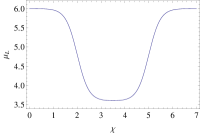
Figure 4: An example of the profile of the chemical potential given in eq.(3.5) with the parameters:  $\mu_{H}=6.0$,  $\kappa=6.5$,  $\delta=3.5$,  $\epsilon=1.5$ and $\lambda=1.2$. Here $\chi$-direction is $S^{1}$ compactified with the period $14$ and $m^{2}=-2$. Although we show two figures here, these are indeed connected in $S^{1}$ circled space, where we assume the branch parts as in Fig.1 locate at $\chi=0$ and $\pm 7$, from which the supercurrents flow in and flow out. Why we show a single profile as two profiles separately is that we perform the analysis for each one independently for the reason mentioned in section 2.2. Here notice that, taking into account the fact that we measure the phases in an anticlockwise direction in Fig.1, the right and the left figures correspond to the chemical potentials in the left and the right parts in the SQUID.

4 The analyses and the results

Taking the chemical potential $\mu$ for each side separately, as in Fig.4, we numerically solve the equations of motion (3.5a)-(3.5) twice with various $J$ as the inputs of the numerical calculation. Namely, our analysis is the one which performs two calculations for a Josephson junction. In our solution, we impose the boundary conditions $M_{t}|_{z=z_{0}}=0$ and that $M_{z}$ is an odd function and $M_{t}$, $M_{\chi}$ and $|\Psi|$ are even functions for $\chi$-direction, where $\chi$-direction is half the space of the whole $\chi$ space, since we perform the calculation for each side of the chemical potential in each side of the circuit of the SQUID separately. To this purpose, we use the spectral method on the Chebyshev Grid [32]. We show examples of the solutions we have obtained in Fig.5.

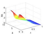
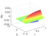
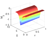
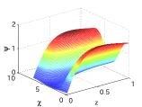
Figure 5: These figures represent examples for the solutions of $M_{t}$, $M_{r}$ $M_{\chi}$ and $|\psi|$ obtained in the parameters as follows: $J/T_{\rm cH}^{2}=1.21316$, the chemical potential (3.5) taken in this calculation is same with the one in the right figure of Fig.4, the Chebyshev Grid is taken as $(n_{z},n_{\chi})=(23,45)$, where $n_{z}$ and $n_{\chi}$ mean number or the grid in $z$- and $\chi$-directions. Here these calculations are performed in the half of the whole $\chi$ space since our calculations are performed for the left and the right parts in the circuit of the SQUID one at a time separately. We show how the sections of the solutions of $|\psi|$ and $M_{\chi}$ at the boundary, $z=0$, in Fig.6, which means the condensation of the cooper pair and $\chi$ component of the gauge field in the dual field theory, respectively.

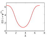
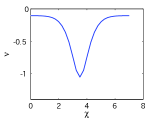
Figure 6: These two figures represent the sections of the solutions of $\overline{\psi}^{(2)}$ and $M_{\chi}$ at the boundary, $z=0$, which mean the condensation of the cooper pair $\langle{\cal O}\rangle$ and $\chi$ component of the gauge field in the dual field theory, respectively.

Finally, we can obtain the numerical results shown in Fig.7, where we list the numerical results of the calculations in Table.1.

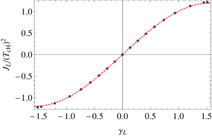
Figure 7: The blue points represent our numerical result obtained from solving the equations of motion (3.5a)-(3.5) with the chemical potential $\mu$ given in the right figure of Fig.4 and various $J_{L}$ as the inputs of the numerical calculations. Here $x$- and $y$-axis show the phase difference $\gamma_{L}$ given in eq.(4.1) and the supercurrent $J_{L}$ normalized by $T_{\rm cH}^{2}$, where $T_{\rm cH}\equiv c~{}\mu_{H}$ with $c\equiv 0.0588$ [13]. The dashed line is the guide line to show that these results are on a sine curve, which is $J_{L}/(T_{\rm cH})^{2}=1.1935\sin(\gamma_{L})$. The result on a sine curve like this figure is one of the specific behaviors in a Josephson junction as mentioned in Section.2.1. We can see that the section of $x$-axis is from about $-\pi/2$ to $\pi/2$.

The dashed line in the figure is the guide for the eye to show that our results are on a sine curve, which is $J_{L}/(T_{\rm cH})^{2}=1.1935\sin(\gamma_{L})$. The result of this sine curve is one of the specific behavior in a Josephson junction as mentioned in Section.2.1.

Here we indicate how to measure the phase difference in this paper. According to Ref.[13], we define the following phase difference for the left and the right sides respectively as

$$\gamma_{L}\equiv\int_{0}^{7}d\chi\left(\nu(\chi)-\nu(0)\right)\quad{\rm and}\quad\gamma_{R}\equiv\int_{-7}^{0}d\chi\left(\nu(\chi)-\nu(-7)\right).$$ (4.1)

Here we have taken into account of the fact that we measure the phases in an anticlockwise direction in the circuit of the SQUID in Fig.1.

Having obtained the result in one Josephson junction, let us turn to the holographic SQUID. The holographic SQUID we consider is composed of two Josephson junctions made from the chemical potential given in Fig.4. To begin with, let us use $J_{L}$ and $J_{R}$ to denote the supercurents flowing in the left and the right sides in the circuit of the SQUID in Fig.1, respectively. Then considering the circuit of the SQUID separately as in Fig.3, we set various values of $J_{L}$ as in Table.1 with a fixed $J_{R}=-0.482052$. Here this $J_{R}$is flowing from the top to the bottom in Fig.1, since we define the $J_{\rm total}$ as in eq.(2.2). Further, such a setting corresponds to the situation where the supercurrent flowing in the left side varies and the supercurrent in the right side flowing constantly.

We have described the validity for giving the values of each supercurrent flowing in the left and the right sides by hand in subsection.2.2. Since the values of the supercurrents are set, the phase differences are determined. Then the magnetic flux $\Phi$ is determined from Table.1 according to eq.(2.3). As a result, from the information of the values of the supercurrents and the magnetic flux, we can read out the relation between the total current $J_{\rm total}$ given in eq.(2.2) and the magnetic flux $\Phi$ induced by the supercurrents flowing in the circuit.

As a result, we can obtain the maximum amplitude of the supercurrent flowing into the circuit $J_{\rm max}$, given in eq.(2.4), against the magnetic flux $\Phi$ as in Fig.8. As can been seen from eq.(2.4), $|J_{\rm max}|$ is to be given as a cosine curve, and the result of the absolute cosine curve like Fig.8 is one of the specific behaviors in the SQUID. Here we can see that Fig.8 has a disparity between the left and the right in the positions of the blue points. The reason for that disparity is simply that our actual numerical data obtained in each Josephson junction, as in Table.1, is from about $-\pi/2$ to $\pi/2$ and the amount of the supercurrent in one side is fixed to a finite value.

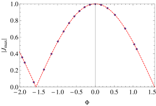
Figure 8: The blue points represent our numerical result for the relation between the magnetic flux $\Phi$ (x-axis) and the absolute value of the maximum amplitude of the supercurrent $|J_{\rm max}|$ flowing into the circuit (y-axis). As can been seen from eq.(2.4), $|J_{\rm max}|$ is to be given as a cosine curve, and the dashed line is the guideline to show that our results are on an absolute cosine curve. The result of an absolute cosine curve like this figure is one of the specific behaviors in the SQUID. In the calculation is the current flowing from the top to the bottom in Fig.1, since we define the $J_{\rm total}$ as in eq.(2.2)), which means that the supercurrent flowing in the left side varies and the supercurrent in the right side flowing constantly. Here we can see the disparity in this figure, which is between the left and the right in the positions of the blue points. The reason for that disparity is simply that the actual numerical data obtained in each Josephson junction, as in Table.1, is from about $-\pi/2$ to $\pi/2$, and the amount of the supercurrent in one side is fixed to a finite value.

Appendix A Damping of the supercurrent in the SQUID

In this appendix, we show that, when closing in on the center of the section in the superconductor part of the SQUID in Fig.1, the flow of the supercurrent diminishes. By this, we show the validity of the ${\bf v}_{s}=0$ in the below eq.(2.3).

To this purpose, taking the orthogonal coordinate system $(x,y,z)$, we assume that the section of the circuit in the superconductor part of the SQUID is put perpendicularly to $y$-direction and parallel with $(x,z)$ plane. Further, we direct $z$-direction parallel to the magnetic flux $\vec{B}\equiv\nabla\times\vec{A}$.

Then from the London equation $\displaystyle\nabla\times\vec{J}_{s}=-\frac{n_{s}e^{*}{}^{2}}{m^{*}}\vec{B}$ and the Maxwell equation $\displaystyle\nabla\times\vec{B}=\vec{J}_{s}$, we can obtain the following equation

$$\nabla^{2}\vec{J}_{s}=\lambda\vec{J}_{s},$$ (A.1)

where $\displaystyle\lambda\equiv\frac{n_{s}e^{*}{}^{2}}{m^{*}}$, and $\vec{J}_{s}$, $m^{*}$, $e^{*}$ and $n_{s}$ are the supercurrent, the mass, the electric charge and the density of the Cooper pair, respectively. Here it turns out that $\displaystyle\vec{J}_{s}=-\frac{n_{s}e^{*}{}^{2}}{m^{*}}\vec{A}$ from the London equation, and, in the derivation of eq.(A.1), we have taken a gauge fixing condition $\displaystyle\nabla\cdot\vec{A}=0$. Then we can obtain the solution as

$$\vec{J}_{s}=e^{-\sqrt{\lambda}x},$$ (A.2)

where the $x$ appearing here is the coordinate for the inside of the section of the SQUID.

Now we can see from the solution shown above, when closing in on the center of the section in the superconductor part of the SQUID, the flow of the supercurrent diminishes. Hence, it is reasonable to consider that the flow of the supercurrent vanishes at the center of the section and ${\bf v}_{s}=0$ as below eq.(2.3).

Appendix B Numerical results used in Figs.7 and 8

We show explicitly the phase difference $\gamma_{L,R}$ defined in eq.(4.1). These are obtained from solving the equations of motion (3.5a)-(3.5) in each left and right space one at a time by varying the value of the supercurrent $J_{L,R}$ as the inputs and taking the chemical potential as in the right figure of Fig.4. Figs.7 and 8 are plotted based on these numerical results. Here let us notice that we measure the phases in an anticlockwise direction in Fig.1 and the relation between $J_{\rm total}$ and $J_{L,R}$ are given eq.(2.2).

$\gamma_{L,R}$	$J_{L,R}/T_{\rm cH}{}^{2}$		$\gamma_{L,R}$	$J_{L,R}/T_{\rm cH}{}^{2}$
-1.51614	-1.21316		0.136253	0.160684
-1.45013	-1.20513		0.274963	0.321368
-1.20955	-1.12479		0.419009	0.482052
-0.939785	-0.964103		0.572359	0.642735
-0.741505	-0.803419		0.741505	0.803419
-0.572359	-0.642735		0.939785	0.964103
-0.419009	-0.482052		1.20955	1.12479
-0.274963	-0.321368		1.45013	1.20513
-0.136253	-0.160684		1.51614	1.21316
0	0

Table 1: The Chebyshev Grid is taken for the all as $(n_{z},n_{\chi})=(20,35)$ except for for the ones of the $J_{L,R}/T_{\rm cH}{}^{2}=\pm 1.21326$. The Chebyshev Grid taken for the ones of the $J_{L,R}/T_{\rm cH}{}^{2}=\pm 1.21326$ is $(n_{z},n_{\chi})=(23,43)$. Here $n_{z}$ and $n_{\chi}$ mean the number or the grid in $z$- and $\chi$-directions, respectively. The critical temperature for the superconductor/normal metal transition $T_{\rm cH}$ is defined as $T_{\rm cH}=c\,\mu_{\rm H}$ with $c\equiv 0.0588$ [13].

References

- [1] J. M. Maldacena, “The Large N limit of superconformal field theories and supergravity,” Adv. Theor. Math. Phys. 2, 231 (1998) [hep-th/9711200].
- [2] S. S. Gubser, I. R. Klebanov and A. M. Polyakov, “Gauge theory correlators from non-critical string theory,” Phys. Lett. B 428, 105 (1998) [arXiv:hep-th/9802109].
- [3] E. Witten, “Anti-de Sitter space and holography,” Adv. Theor. Math. Phys. 2, 253 (1998) [arXiv:hep-th/9802150].
- [4] S. S. Gubser, “Breaking an Abelian gauge symmetry near a black hole horizon,” Phys. Rev. D 78, 065034 (2008) [arXiv:0801.2977 [hep-th]].
- [5] S. A. Hartnoll, C. P. Herzog and G. T. Horowitz, “Building a Holographic Superconductor,” Phys. Rev. Lett. 101, 031601 (2008) [arXiv:0803.3295 [hep-th]].
- [6] S. A. Hartnoll, C. P. Herzog and G. T. Horowitz, “Holographic Superconductors,” JHEP 0812, 015 (2008) [arXiv:0810.1563 [hep-th]].
- [7] S. -S. Lee, “A Non-Fermi Liquid from a Charged Black Hole: A Critical Fermi Ball,” Phys. Rev. D 79, 086006 (2009) [arXiv:0809.3402 [hep-th]].
- [8] H. Liu, J. McGreevy and D. Vegh, “Non-Fermi liquids from holography,” Phys. Rev. D 83, 065029 (2011) [arXiv:0903.2477 [hep-th]].
- [9] M. Cubrovic, J. Zaanen and K. Schalm, “String Theory, Quantum Phase Transitions and the Emergent Fermi-Liquid,” Science 325, 439 (2009) [arXiv:0904.1993 [hep-th]].
- [10] T. Nishioka, S. Ryu and T. Takayanagi, “Holographic Superconductor/Insulator Transition at Zero Temperature,” JHEP 1003, 131 (2010) [arXiv:0911.0962 [hep-th]].
- [11] R. G. Cai, L. Li, L. F. Li and R. Q. Yang, “Introduction to Holographic Superconductor Models,” arXiv:1502.00437 [hep-th].
- [12] B. D. Josephson, Possible new effects in superconductive tunnelling, Phys. Lett. 1, 251 (1962).
- [13] G. T. Horowitz, J. E. Santos and B. Way, A Holographic Josephson Junction, Phys. Rev. Lett. 106, 221601 (2011) [arXiv:1101.3326 [hep-th]].
- [14] Y. -Q. Wang, Y. -X. Liu and Z. -H. Zhao, “Holographic Josephson Junction in 3+1 dimensions,” arXiv:1104.4303 [hep-th].
- [15] M. Siani, “On inhomogeneous holographic superconductors,” arXiv:1104.4463 [hep-th].
- [16] Y. -Q. Wang, Y. -X. Liu and Z. -H. Zhao, “Holographic p-wave Josephson junction,” arXiv:1109.4426 [hep-th].
- [17] Y. -Q. Wang, Y. -X. Liu, R. -G. Cai, S. Takeuchi and H. -Q. Zhang, “Holographic SIS Josephson Junction,” JHEP 1209, 058 (2012) [arXiv:1205.4406 [hep-th]].
- [18] E. Kiritsis and V. Niarchos, “Josephson Junctions and AdS/CFT Networks,” JHEP 1107, 112 (2011) [Erratum-ibid. 1110, 095 (2011)] [arXiv:1105.6100 [hep-th]].
- [19] H. F. Li, L. Li, Y. Q. Wang and H. Q. Zhang, “Non-relativistic Josephson Junction from Holography,” JHEP 1412, 099 (2014) [arXiv:1410.5578 [hep-th]].
- [20] E. Nakano and W. -Y. Wen, “Critical magnetic field in a holographic superconductor,” Phys. Rev. D 78, 046004 (2008) [arXiv:0804.3180 [hep-th]].
- [21] T. Albash and C. V. Johnson, “A Holographic Superconductor in an External Magnetic Field,” JHEP 0809, 121 (2008) [arXiv:0804.3466 [hep-th]].
- [22] S. A. Hartnoll and P. Kovtun, “Hall conductivity from dyonic black holes,” Phys. Rev. D 76, 066001 (2007) [arXiv:0704.1160 [hep-th]].
- [23] O. Domenech, M. Montull, A. Pomarol, A. Salvio and P. J. Silva, “Emergent Gauge Fields in Holographic Superconductors,” JHEP 1008, 033 (2010) [arXiv:1005.1776 [hep-th]].
- [24] M. Montull, O. Pujolas, A. Salvio and P. J. Silva, “Flux Periodicities and Quantum Hair on Holographic Superconductors,” Phys. Rev. Lett. 107, 181601 (2011) [arXiv:1105.5392 [hep-th]].
- [25] A. Salvio, “Superconductivity, Superfluidity and Holography,” J. Phys. Conf. Ser. 442, 012040 (2013) [arXiv:1301.0201].
- [26] M. Montull, O. Pujolas, A. Salvio and P. J. Silva, “Magnetic Response in the Holographic Insulator/Superconductor Transition,” JHEP 1204, 135 (2012) [arXiv:1202.0006 [hep-th]].
- [27] R. -G. Cai, L. Li, L. -F. Li, H. -Q. Zhang and Y. -L. Zhang, “Wilson Line Response of Holographic Superconductors in Gauss-Bonnet Gravity,” Phys. Rev. D 87, 026002 (2013) [arXiv:1209.5049 [hep-th]].
- [28] Pasi Lhteenmki, G. S. Paraoanu, Juha Hassel, Pertti J. Hakonen, “Dynamical Casimir effect in a Josephson metamaterial,” Proc. Natl. Acad. Sci. U.S.A. 110, 4234 (2013) [arXiv:1111.5608].
- [29] R. -G. Cai, Y. -Q. Wang and H. -Q. Zhang, “A holographic model of SQUID,” arXiv:1308.5088 [hep-th].
- [30] G. T. Horowitz and R. C. Myers, “The AdS / CFT correspondence and a new positive energy conjecture for general relativity,” Phys. Rev. D 59, 026005 (1998) [hep-th/9808079].
- [31] S. Nakamura, “Comments on Chemical Potentials in AdS/CFT,” Prog. Theor. Phys. 119, 839 (2008) [arXiv:0711.1601 [hep-th]].
- [32] Lloyd N. Trefethen, Spectral Methods in MATLAB, SIAM, Philadelphia, 2000.