Accessing interior magnetic field vector components in neutron electric dipole moment experiments via exterior measurements
I. Boundary-value techniques

Abstract

We propose a new concept for determining the interior magnetic field vector components in neutron electric dipole moment experiments. If a closed three-dimensional boundary surface surrounding the fiducial volume of an experiment can be defined such that its interior encloses no currents or sources of magnetization, each of the interior vector field components and the magnetic scalar potential will satisfy a Laplace equation. Therefore, if either the vector field components or the normal derivative of the scalar potential can be measured on the surface of this boundary, thus defining a Dirichlet or Neumann boundary-value problem, respectively, the interior vector field components or the scalar potential (and, thus, the field components via the gradient of the potential) can be uniquely determined via solution of the Laplace equation. We discuss the applicability of this technique to the determination of the interior magnetic field components during the operating phase of neutron electric dipole moment experiments when it is not, in general, feasible to perform direct in situ measurements of the interior field components. We also study the specifications that a vector field probe must satisfy in order to determine the interior vector field components to a certain precision. The technique we propose here may also be applicable to experiments requiring monitoring of the vector magnetic field components within some closed boundary surface, such as searches for neutron-antineutron oscillations along a flight path or measurements in storage rings of the muon anomalous magnetic moment $g-2$ and the proton electric dipole moment.

1 Introduction

The basic principle upon which all experimental searches for a neutron electric dipole moment (EDM) employing stored ultracold neutrons (UCN) are based concerns measurements of the neutrons’ Larmor spin precession frequencies $\nu_{\pm}$ in parallel ($+$) and anti-parallel ($-$) magnetic ($\vec{B}$) and electric ($\vec{E}$) fields,

$$h\nu_{\pm}=-2\left(\mu_{n}|\vec{B}|\pm d_{n}|\vec{E}|\right).$$ (1)

Here, $\mu_{n}$ and $d_{n}$ denote the neutron’s magnetic and electric dipole moments, respectively. A value for, or a limit on, $d_{n}$ is then deduced from a comparison of the measured values of $\nu_{+}$ and $\nu_{-}$. The frequencies $\nu_{+}$ and $\nu_{-}$ are typically determined either from sequential measurements in a single volume, or from simultaneous measurements in separate volumes. Therefore, a central problem to all neutron EDM experiments concerns the determination of the value of the magnetic field averaged over the single or separate volumes, especially in the presence of temporal fluctuations and/or spatial variations in the field [1]. An elegant solution providing for real-time monitoring of the magnetic field is to deploy a so-called “co-magnetometer”, whereby an atomic species with no EDM (or, at least, one known to be significantly smaller than the neutron EDM) co-habitates together with the stored UCN the fiducial volume [2, 3, 4, 5, 6]. The general idea is then to carry out a measurement of the co-magnetometer atoms’ Larmor spin precession frequency in the magnetic field, from which the temporal dependence of the scalar magnitude of the magnetic field $|\vec{B}|$ averaged over the fiducial volume is then deduced.

Thus, a co-magnetometer provides for a real-time, in situ measurement of the scalar magnitude $|\vec{B}|$, which is especially important for detecting any shifts in $|\vec{B}|$ correlated with the reversal of the direction of $\vec{E}$ relative to $\vec{B}$. However, there are many optimization parameters and systematic effects in neutron EDM experiments associated with the vector components of the magnetic field, $B_{i}$, or, equivalently, the field gradients $\partial B_{i}/\partial x_{j}$. For example, the longitudinal and transverse spin relaxation times, $T_{1}$ and $T_{2}$, the values of which contribute to a determination of an experiment’s statistical figure-of-merit, depend, among other parameters, on the field gradients [7, 8, 9, 10, 11, 12]. As another example, the dominant systematic uncertainty in the most recent published limit on $d_{n}$ [13] resulted from the so-called “geometric phase” false EDMs of the neutron and the co-magnetometer atoms [14, 15, 16, 17, 18, 19], both of which are functions of the field gradients.

Despite the importance of knowledge of the field gradients in neutron EDM experiments, the key point here is that a co-magnetometer does not, in general, provide for a real-time, in situ measurement of the $\partial B_{i}/\partial x_{j}$ field gradients. Nor is it practical or feasible to carry out direct in situ measurements of the field components or field gradients in an experiment’s fiducial volume with some probe after the experimental apparatus has been assembled. However, the situation is not that grim, as it has been shown that it may be possible to extract some particular field gradients from measurements of the spin relaxation times coupled with measurements of the neutrons’ and co-magnetometer atoms’ trajectory correlation functions [18], and also (under various assumptions on the symmetry properties of the magnetic field profile) from a comparison of the neutron’s and co-magnetometer atoms’ precession frequencies and their center-of-mass positions in the magnetic field [14, 6].

The concept we propose to employ for a real-time determination of the interior vector field components $B_{i}$, and thus the field gradients $\partial B_{i}/\partial x_{j}$, is a completely general method based on boundary-value techniques which does not require any assumptions on the symmetry properties (or lack thereof) of the field. The basic idea is to perform measurements of the field components on the surface of a boundary surrounding the experiment’s fiducial volume, and then solve (uniquely) for the values of the field components in the region interior to this boundary via standard numerical methods. Although the physics basis of the concepts we discuss in this paper are certainly not original (and likely known since the origins of electromagnetic theory), to our knowledge this concept has not been suggested for use in a neutron EDM experiment, although it certainly has been suggested in other contexts (e.g., [20]); nevertheless, we believe the discussion in this paper will be of value to those engaged in neutron EDM experiments. The remainder of this paper is organized as follows. In Secs. 2 and 3 we discuss the boundary-value problem under consideration and its applicability to neutron EDM experiments. We then show examples from numerical studies of this problem in Sec. 4 for the geometry of the neutron EDM experiment to be conducted at the Spallation Neutron Source [21], the concept of which is based on the pioneering ideas of Golub and Lamoreaux [4]. We then study the specifications (e.g., precision) on a vector field probe in Sec. 5. Finally, we conclude with a brief summary in Sec. 6.

2 Boundary-Value Problem for the Interior Vector Field Components

2.1 Statement of the Boundary-Value Problem

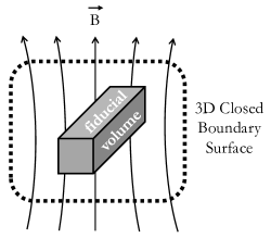
Figure 1: Schematic illustration of the proposed boundary-value problem for the determination of the magnetic field vector components interior to a three-dimensional closed surface surrounding an experiment’s fiducial volume.

We begin by considering, as shown schematically in Fig. 1, a closed three-dimensional boundary surface surrounding the fiducial volume of an experiment, which is situated within an arbitrary magnetic field (i.e., no assumptions on the symmetry properties of the field are necessary). Our starting point is the fundamental equations of magnetostatics, which in SI units are $\vec{\nabla}\times\vec{H}=\vec{J}$ and $\vec{\nabla}\cdot\vec{B}=0$, where $\vec{B}=\mu_{0}(\vec{H}+\vec{M})$. If we assume that the volume enclosed by the boundary surface contains: (1) no sources of currents, such that that the current density $\vec{J}=0$ everywhere inside of the boundary; and (2) no sources of magnetization, such that the magnetization $\vec{M}=0$ everywhere inside of the boundary, it then follows that $\vec{\nabla}\times\vec{B}=0$. From this, we immediately see, via application of the general vector identity $\vec{\nabla}\times(\vec{\nabla}\times\vec{B})=\vec{\nabla}(\vec{\nabla}\cdot\vec{B})-\vec{\nabla}^{2}\vec{B}$, that the magnetic field $\vec{B}$ (and, thus, each of its components $B_{i}$) satisfies a Laplace equation,

$$\vec{\nabla}^{2}\vec{B}=0~{}~{}\Longrightarrow~{}~{}\vec{\nabla}^{2}B_{i}=0~{}~{}(i=x,y,z),$$ (2)

everywhere inside of the boundary.

Alternatively, under the above assumptions that $\vec{\nabla}\times\vec{B}=0$ and $\vec{\nabla}\cdot\vec{B}=0$ everywhere inside of the boundary, in a manner analogous to charge-free electrostatics (i.e., $\vec{\nabla}\times\vec{E}=0$ and $\vec{\nabla}\cdot\vec{E}=0$) we can define a magnetic scalar potential $\Phi_{M}$ which satisfies $\vec{B}=-\vec{\nabla}\Phi_{M}$. From this, it then immediately follows that imposing the requirement $\vec{\nabla}\cdot\vec{B}=0$ leads to a Laplace equation for the scalar potential,

$$\vec{\nabla}^{2}\Phi_{M}=0,$$ (3)

everywhere inside of the boundary.

Therefore, in summary, we see that each of the vector field components $B_{i}$ and the scalar potential $\Phi_{M}$ satisfy a Laplace equation everywhere inside of the boundary, provided the boundary encloses no current or magnetization. Solutions to the Laplace equation, subject to boundary values, are well known (e.g., [22]); thus, determination of the interior field components or the scalar potential from exterior boundary-value measurements is a solvable problem.

2.2 Dirichlet Problem for the Interior Vector Components

We now consider the Laplace equation for one of the vector components, $\vec{\nabla}^{2}B_{i}=0$. If boundary values for $B_{i}$ are known everywhere on the surface of the boundary, the interior values of $B_{i}$ everywhere inside the surface of the boundary can, in principle, be obtained from an integral equation over the boundary values and the appropriate Dirichlet Green’s function for the geometry in question. Thus, for the continuous version of the Dirichlet boundary-value problem posed here, it is theoretically possible to solve for the interior vector components everywhere inside the boundary, provided their boundary values are known everywhere on the surface. Such a solution will be unique [22]. Note that a limitation of the Dirichlet problem we have formulated is that it requires boundary values for the same component $B_{i}$ everywhere on the surface, with the solution to the problem only yielding interior values for $B_{i}$ (i.e., no information on $B_{j}$ where $j\neq i$ can be deduced).

2.3 Neumann Problem for the Interior Magnetic Scalar Potential

Next we consider the Laplace equation for the magnetic scalar potential, $\vec{\nabla}^{2}\Phi_{M}=0$. The scalar potential $\Phi_{M}$ is, of course, not a physical observable; however, the vector components of the gradient, $\vec{B}=-\vec{\nabla}\Phi_{M}$, are, of course, physical observables. Let $\hat{n}$ denote a unit vector normal to the surface of the boundary. If we then assume that boundary values for the normal derivative of the scalar potential, $\partial\Phi_{M}/\partial n=\vec{\nabla}\Phi_{M}\cdot\hat{n}$, or, equivalently, the negative of the normal component of the magnetic field, $-B_{n}=\partial\Phi_{M}/\partial n$, are known everywhere on the surface of the boundary, the interior values of $\Phi_{M}$ can, in principle, be obtained from an integral equation over the boundary values and the appropriate Neumann Green’s function for the geometry in question. Thus, for the continous version of the Neumann boundary-value problem posed here, it is theoretically possible to solve for the interior scalar potential everywhere inside the boundary, provided the normal components of the magnetic field are known everywhere on the surface. Unlike the Dirichlet problem, the solution to the Neumann problem for the interior scalar potential will not be unique, as the value of the scalar potential is arbitrary up to a constant $\Phi_{M}\rightarrow\Phi_{M}+\lambda$ [22]; however, the resulting interior magnetic field components, $\vec{B}=-\vec{\nabla}\Phi_{M}$, will be unique. Note that in contrast to the Dirichlet problem, the solution to the Neumann problem determines all of the interior vector components of $\vec{B}$.

2.4 Comment on Exterior Measurements of $|\vec{B}|$

Exterior measurements (i.e., outside the fiducial volume) of the scalar magnitude of the magnetic field, $|\vec{B}|$, are certainly useful as they provide for important monitoring of the magnetic field in the vicinity of the fiducial volume. However, we note that such measurements do not provide for a rigorous determination of either the interior scalar magnitude $|\vec{B}|$ or the interior vector components of $\vec{B}$, as the scalar magnitude $|\vec{B}|$ does not satisfy a Laplace equation. Therefore, any attempt to extract information on the interior $\partial B_{i}/\partial x_{j}$ field gradients from exterior measurements of $|\vec{B}|$ will necessarily require various assumptions to be made on the symmetry properties of the magnetic field. In particular, fitting exterior measurements of $|\vec{B}|$ to a multipole expansion in spherical harmonics in order to determine interior values of $|\vec{B}|$ is not completely rigorous, as such a multipole expansion is the solution for a quantity which necessarily obeys the Laplace equation.

3 Discretization of the Boundary-Value Problem

3.1 Discretization of the Geometry

In the (hypothetical) continuous versions of the Dirichlet and Neumann boundary-value problems formulated above, it was assumed that the boundary values were known everywhere on the surface; this leads to the well-known analytic solutions for the interior values in terms of integral equations of Green’s functions. Of course, such a problem cannot be realized in practice, as the boundary values can only be determined at discrete measurement points. Fortunately, numerical solutions to discretized versions of the Dirichlet and Neumann boundary-value problems are well known (e.g., [23]).

In the discretized versions of the boundary-value problems we will consider hereafter, we will assume, as indicated schematically in Fig. 2, that the boundary values (i.e., $B_{i}$ for the Dirichlet problem or $B_{n}$ for the Neumann problem) are known over a regularly-spaced grid on the surface of the boundary, with the (constant) spacing between adjacent points along the $x$, $y$, and $z$ directions denoted $\Delta x$, $\Delta y$, and $\Delta z$. Note that it is not necessary to employ uniform $\Delta x=\Delta y=\Delta z$ grid spacings. Also, it is not necessary to employ “flat” boundary surfaces, such as the sides of a rectangular box, although, for simplicity, the illustrative examples we will consider in the next section do utilize a rectangular box geometry. For example, one could discretize the surface of a torus, which would be a natural candidate for a boundary surface surrounding the interior of an experiment located within a circular accelerator storage ring.

Finally, it is also worthwhile to note that the boundary-value problem must be cast in three dimensions. For example, the solution to the Laplace equation $\vec{\nabla}^{2}B_{i}=0$ need not satisfy $(\frac{\partial^{2}}{\partial x^{2}}+\frac{\partial^{2}}{\partial y^{2}})B_{i}=0$ in two dimensions. Therefore, an attempt to simplify the Dirichlet and Neumann boundary-value problems for $B_{i}$ and $\Phi_{M}$, respectively, from three to two dimensions will not, in general, yield a valid solution.

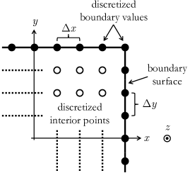
Figure 2: Schematic illustration in two dimensions of the discretized version of the boundary-value problem; the extension to three dimensions is obvious. Space is discretized into grid points, with constant separations $\Delta x$, $\Delta y$, and $\Delta z$ along their respective directions. The boundary values are assumed to be known over a grid of points on the surface of the boundary (filled circles). The solution is then desired over the grid of interior points (open circles).

3.2 Methods for Numerical Solution of the Laplace Equation

In general, there exists a multitude of techniques for the numerical solution of the Laplace equation subject to boundary values (see, e.g., [23]), and we do not endeavor to discuss these techniques here. We employed the finite differencing method of relaxation (examples of techniques include Jacobi iteration, Gauss-Seidel iteration, successive overrelaxation, etc.), with the results in the next section obtained using approximations to the second-order partial derivatives valid to $\mathcal{O}((\Delta x)^{2})$, i.e.,

$$\left.\frac{\partial^{2}u}{\partial x^{2}}\right|_{(i,j,k)}=\frac{u(i+1,j,k)-2u(i,j,k)+u(i-1,j,k)}{(\Delta x)^{2}}.$$ (4)

Here the notation $u(i,j,k)$ denotes the solution to the Laplace equation $\vec{\nabla}^{2}u(x,y,z)=0$ at some $(x,y,z)$ grid point indexed by the integers $(i,j,k)$. Note that to this order, if one takes $\Delta x=\Delta y=\Delta z$, one obtains the well-known result for $u(i,j,k)$ in terms of the values of the solution at its six nearest neighbor grid points,

$$u(i,j,k) = \frac{1}{6}\Big{[}u(i+1,j,k)+u(i-1,j,k)+u(i,j+1,k)+u(i,j-1,k)$$ (5)

$$~{}~{}~{}+u(i,j,k+1)+u(i,j,k-1)\Big{]}.$$

4 Examples from Numerical Studies

4.1 Geometry and Magnetic Field

As a validation of our concept, we now show results from numerical studies of the Dirichlet boundary-value problem for $B_{i}$ and the Neumann boundary-value problem for $\Phi_{M}$. The example geometry we will consider is that of the neutron EDM experiment to be conducted at the Spallation Neutron Source [21]. In particular, this geometry consists of two rectangular measurement volumes, which together span our definition of a rectangular fiducial volume of dimensions 25 cm ($-12.5$ cm $<x<$ $12.5$ cm) $\times$ 10 cm ($-5.0$ cm $<y<$ $5.0$ cm) $\times$ 40 cm ($-20.0$ cm $<z<$ $20.0$ cm). We then employ a rectangular boundary surface of dimensions 80 cm ($-40.0$ cm $<x<$ $40.0$ cm) $\times$ 80 cm ($-40.0$ cm $<y<$ $40.0$ cm) $\times$ 100 cm ($-50.0$ cm $<z<$ $50.0$ cm). Thus, the volume enclosed by the boundary surfaces is significantly larger (factor of 64) than the fiducial volume, with the boundary surfaces all located $\sim 30$ cm from the fiducial volume.

The magnetic field we will consider is a calculated field map of a modified $\cos\theta$ coil under development for this particular experiment [24]. The orientation of the $\cos\theta$ coil is such that the fiducial volume is centered on the coil’s center, with the magnetic field $\vec{B}$ oriented along the $x$-direction at the center of the fiducial volume.

4.2 Example Dirichlet Problem: Densely-Spaced Boundary Values

As our first numerical example, we considered a Dirichlet boundary-value problem for each of the $(B_{x},B_{y},B_{z})$ field components in a geometry where the spacing between the grid points is $\Delta x=\Delta y=\Delta z=1.0$ cm, thus resulting in 44,802 densely-spaced grid points on the surface of the boundary. As per the discussion in Sec. 3, we assumed the values of $(B_{x},B_{y},B_{z})$ were known at all of the 44,802 boundary grid points. We then proceeded to solve for the values of $(B_{x},B_{y},B_{z})$ at all of the 617,859 interior grid points. The computing time required for $10^{5}$ iterations of our C++ code on a Linux machine was 93 minutes. Obviously, implementing such a densely-spaced configuration would not be possible or practical in an actual experiment; instead, the point of this hypothetical example was to first demonstrate the validity of the boundary-value technique for the determination of the interior field components.

Figure 3: Results from numerical studies of the Dirichlet boundary-value problem for $B_{i}$ for the densely-spaced grid of $\Delta x=\Delta y=\Delta z=1.0$ cm (see text for details). Calculated interior values for $B_{x}$ along the $x$-, $y$-, and $z$-axes are shown in panels (a), (b), and (c) as the filled circles, and are compared with the exact values shown as the solid curves. Panel (d) shows a histogram of the fractional error in the calculated interior values of $(B_{x},B_{y},B_{z})$ for all of the interior grid points.

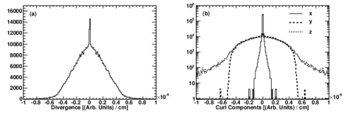
Figure 4: Histograms of values for $\vec{\nabla}\cdot\vec{B}$ in panel (a) and the $x$-, $y$-, and $z$-components of $\vec{\nabla}\times\vec{B}$ in panel (b) for the calculated interior values of $B_{i}$ at all of the interior grid points from the Dirichlet boundary-value problem for the densely-spaced grid of $\Delta x=\Delta y=\Delta z=1.0$ cm (see text for details).

The results of this exercise are shown in Fig. 3. Panels (a), (b), and (c) compare the calculated interior values of $B_{x}$ along the $x$-, $y$-, and $z$-axes with the exact values from the field map, and panel (d) then shows histograms of the fractional errors [defined to be (calculated $-$ exact)/exact] in the calculated interior values of $(B_{x},B_{y},B_{z})$ at all of the interior points. The agreement between the calculated and exact values is seen to be excellent, thus clearly demonstrating the validity of our proposed concept. As a further check, Fig. 4 shows histograms of values for $\vec{\nabla}\cdot\vec{B}$ and $\vec{\nabla}\times\vec{B}$ determined from the calculated interior values (using the centered difference approximation). As expected, the distributions are centered on zero, consistent with the initial assumptions of the problem.

4.3 Example Neumann Problem: Densely-Spaced Boundary Values

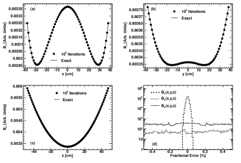
Figure 5: Results from numerical studies of the Neumann boundary-value problem for $\Phi_{M}$ and resulting values for $\vec{B}=-\vec{\nabla}\Phi_{M}$ for the densely-spaced grid of $\Delta x=\Delta y=\Delta z=1.0$ cm (see text for details). Values for $B_{x}=-\partial\Phi_{M}/\partial x$ along the $x$-, $y$-, and $z$-axes as calculated from the interior values for $\Phi_{M}$ are shown in panels (a), (b), and (c) as the filled circles, and are compared with the exact values shown as the solid curves. Panel (d) shows a histogram of the fractional error in the calculated interior values of $(B_{x},B_{y},B_{z})$ for all of the interior grid points.

We now consider the Neumann boundary-value problem for $\Phi_{M}$ for the same densely-spaced grid configuration employed in the discussion of the Dirichlet boundary-value problem in Section 4.2. Again, as per the discussion in Sec. 3, we assumed the values of $-B_{n}=\partial\Phi_{M}/\partial n$ were known at all of the boundary grid points. We then proceeded to solve for the values of $\Phi_{M}$ at all of the interior grid points. The computing time required for $10^{5}$ iterations of our C++ code on a Linux machine for the solution of the Neumann problem for $\Phi_{M}$ was 24 minutes, a little better than 1/3 of that required for solution of the Dirichlet problem for all three components of $\vec{B}$.

The results of this exercise are shown in Fig. 5. As before, panels (a), (b), and (c) compare the calculated interior values of $B_{x}=-\partial\Phi_{M}/\partial x$ with the exact values from the field map, and panel (d) then shows histograms of the fractional errors in the calculated interior values of $(B_{x},B_{y},B_{z})$ for all of the interior grid points. Again, the agreement between the calculated and exact values for $B_{x}$ (i.e., the dominant field component) is excellent, again clearly demonstrating the validity of the Neumann concept. However, the fractional errors in the calculated values of $B_{y}$ and $B_{z}$ are larger than those for $B_{x}$; this is the result of a loss of precision in calculating these significantly smaller components via derivatives of $\Phi_{M}$.

4.4 Example Dirichlet Problem: Coarsely-Spaced Boundary Values

We now consider more realistic examples of the Dirichlet boundary-value problem in which the grids are (significantly) more coarsely spaced than those of the previous examples. First, calculated interior values of $B_{x}$ along the $x$-axis are shown in panel (a) of Fig. 6 for a grid with spacings $(\Delta x,\Delta y,\Delta z)$ = (10 cm, 10 cm, 50 cm), which would require measurements of 194 boundary values. The agreement between the calculated and exact values is still quite good. Second, panel (b) shows results from the same calculation for an even coarser grid with spacings $(\Delta x,\Delta y,\Delta z)$ = (10 cm, 40 cm, 50 cm), requiring measurements of 74 boundary values. The agreement is now somewhat degraded, although the calculated and exact values still agree to the level of $\sim 0.08$%. A drawback of this latter coarse grid is that the number of interior points are limited to those shown in panel (b) because $\Delta y$ and $\Delta z$ are simply half of the extent of the fiducial volume in their respective directions.

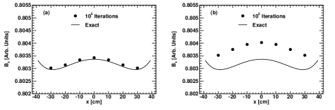
Figure 6: Results from numerical studies of the Dirichlet boundary-value problem for $B_{i}$ for two coarsely spaced boundary value grids. Panel (a) shows calculated interior values of $B_{x}$ along the $x$-axis (filled circles) compared with the exact values (solid curves) for a grid with $(\Delta x,\Delta y,\Delta z)$ = (10 cm, 10 cm, 50 cm). Panel (b) is for a grid with $(\Delta x,\Delta y,\Delta z)$ = (10 cm, 40 cm, 50 cm). Note that we do not show values for $B_{x}$ along the $y$- or $z$-axes, as there are very few interior grid points along these dimensions given the relatively large $\Delta y$ and $\Delta z$ grid spacings.

The computing time required for $10^{5}$ iterations of our codes was $<10$ seconds for both of these coarse grids.

5 Specifications on the Vector Field Probe

Measurements of boundary values in an experiment with a vector field probe will, of course, be subject to noise and/or systematic errors such as uncertainties in the probe’s $(x,y,z)$ positioning or its calibration. To study the specifications that a probe must satisfy in order to determine the interior field components to a certain precision, we employ a simple model in which we subject each boundary value $B_{i}$ to a Gaussian fluctuation parameter $\delta$,

$$B_{i}\rightarrow B_{i}(1+\delta),$$ (6)

where $\delta$ is randomly sampled from a Gaussian with a mean of zero and a particular width $\sigma$. This simple model accounts for noise fluctuations in the measurement of $B_{i}$ and also errors in the probe’s $(x,y,z)$ positioning, the latter of which can be interpreted as equivalent to an error in the measurement at the nominal $(x,y,z)$ position.

We considered two examples of $\sigma=10^{-3}$ and $10^{-4}$ which we illustrate within the context of the two coarse grids discussed previously in Section 4.4 (i.e., those with $(\Delta x,\Delta y,\Delta z)$ = (10 cm, 10 cm, 50 cm) and (10 cm, 40 cm, 50 cm), yielding 194 and 74 boundary values, respectively). To provide context for an experiment, a $\sigma$ of $10^{-4}$ would correspond to a Gaussian width of $10^{-6}$ Gauss on a $10^{-2}$ Gauss field value, where $10^{-2}$ Gauss is the typical scale of field magnitudes in recent and future neutron EDM experiments. For each of these $\sigma$ values, we generated ten random configurations of boundary values in which each of the boundary values was subjected to a Gaussian fluctuation according to Eq. (6). The impact of these fluctuations on the calculated interior values is shown in Fig. 7, where we show the calculated interior values of $B_{x}$ along the $x$-axis for each of the ten random configurations. As can be seen there, if $\sigma=10^{-3}$ the spread in the calculated interior values is rather large (and the sign of the gradient $\partial B_{x}/\partial x$ that would be deduced would be incorrect in some cases), whereas if $\sigma=10^{-4}$ the spread is small and any differences in the values of $\partial B_{x}/\partial x$ deduced from the calculated interior values would be small.

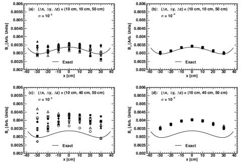
Figure 7: Results from numerical studies of the impact of noise and/or systematic errors in the measurements of the boundary values on the calculated interior values. All panels show calculated interior values of $B_{x}$ along the $x$-axis for ten random configurations of boundary values (indicated by the different data symbols) generated according to the Gaussian fluctuation model discussed in the text. Panel (a): grid spacing of $(\Delta x,\Delta y,\Delta z)$ = (10 cm, 10 cm, 50 cm) and Gaussian fluctuation parameter $\sigma=10^{-3}$. Panel (b): (10 cm, 10 cm, 50 cm) and $\sigma=10^{-4}$. Panel (c): (10 cm, 40 cm, 50 cm) and $\sigma=10^{-3}$. Panel (d): (10 cm, 40 cm, 50 cm) and $\sigma=10^{-4}$. In panels (b) and (d) the different data symbols all overlap each other.

Thus, within the context of this simple model, we conclude that a reasonable specification on a vector field probe is that the relative uncertainties in the probes’ measurements of the boundary values must be of order $10^{-4}$ and any errors in the $(x,y,z)$ positioning of the probes must not result in measured field values that differ by more than $10^{-4}$ from what their values would be at their nominal positions.

6 Summary

In summary, we have proposed a new concept for determining the interior magnetic field vector components in neutron EDM experiments via Dirichlet and Neumann boundary-value techniques, whereby exterior measurements of the field components over a closed boundary surface surrounding the experiment’s fiducial volume uniquely determine the interior field components via solution of the Laplace equation. We suggest that this technique will be of particular use to neutron EDM experiments after they have been assembled and are in operation, when it is no longer possible to perform an in-situ field map.

We also emphasize that this technique is certainly not limited in its applicability to neutron EDM experiments. Indeed, this technique could be of interest of any experiment requiring monitoring of vector field components within some well defined boundary surface. Some examples of this could be experimental searches for neutron-antineutron ($n\overline{n}$) oscillations along a flight path or experiments utilizing storage rings for measurements of the muon $g-2$ or the proton EDM. The concept for an $n\overline{n}$ experiment would be to mount field probes along the neutron flight path in the region interior to the magnetic shielding, and for the storage ring experiments on the beam vacuum pipe in the region interior to the storage ring magnets and electrodes.

However, as relevant for neutron EDM experiments, we do note that one limitation of our boundary-value concept was discussed in Sec. 4.4: that is, the number of interior points at which the interior fields can be calculated (and, thus, the resolution at which the field gradients can be determined) is limited by the number of grid points (or, equivalently, the grid spacing) at which the boundary values are measured. In a forthcoming work [25], we will explore an alternative technique of fitting measurements of exterior field components to a multipole expansion of the field components or the magnetic scalar potential. Such a technique is valid because the field components and the scalar potential satisfy the Laplace equation, and an expansion in multipoles is a valid solution to the Laplace equation. This technique, via the nature of a “fit” (as compared to the direct solution of the Laplace equation in the boundary-value technique discussed in the present work), holds the potential for a determination of the interior field components everywhere within the fiducial volume.

Acknowledgments
We thank M. P. Mendenhall for providing the field map of the $\cos\theta$ coil we used in our example calculations. We thank C. Crawford, B. Filippone, R. Golub, and J. Miller for several valuable suggestions regarding the development of the concept, R. W. Pattie, Jr. for suggesting the possible applicability of the concept to $n\overline{n}$ experiments, and R. Golub, M. E. Hayden, S. K. Lamoreaux, and N. Nouri for comments on the manuscript. This work was supported in part by the U. S. Department of Energy Office of Nuclear Physics under Award No. DE-FG02-08ER41557.

References

- [1] S. K. Lamoreaux and R. Golub, J. Phys. G 36, 104002 (2009).
- [2] K. Green et al., Nucl. Instrum. Methods Phys. Res. A 404, 381 (1998).
- [3] C. A. Baker et al., arXiv:1305.7336.
- [4] R. Golub and S. K. Lamoreaux, Phys. Rep. 237, 1 (1994).
- [5] I. Altarev et al., Nucl. Instrum. Methods Phys. Res. A 611, 133 (2009).
- [6] Y. Masuda et al., Phys. Lett. A 376, 1347 (2012).
- [7] R. L. Gamblin and T. R. Carver, Phys. Rev. 138, A946 (1965).
- [8] L. D. Schearer and G. K. Walters, Phys. Rev. 139, A1398 (1965).
- [9] G. D. Cates, S. R. Schaefer, and W. Happer, Phys. Rev. A 37, 2877 (1988).
- [10] G. D. Cates, D. J. White, T.-R. Chien, S. R. Schaefer, and W. Happer, Phys. Rev. A 38, 5092 (1988).
- [11] D. D. McGregor, Phys. Rev. A 41, 2631 (1990).
- [12] R. Golub, R. M. Rohm, and C. M. Swank, Phys. Rev. A 83, 023402 (2011).
- [13] C. A. Baker et al., Phys. Rev. Lett. 97, 131801 (2006).
- [14] J. M. Pendlebury et al., Phys. Rev. A 70, 032102 (2004).
- [15] P. G. Harris and J. M. Pendlebury, Phys. Rev. A 73, 014101 (2006).
- [16] S. K. Lamoreaux and R. Golub, Phys. Rev. A 71, 032104 (2005).
- [17] A. L. Barabanov, R. Golub, and S. K. Lamoreaux, Phys. Rev. A 74, 052115 (2006).
- [18] R. Golub and C. M. Swank, arXiv:0810.5378.
- [19] H. Yan and B. Plaster, Nucl. Instrum. Methods Phys. Res. A 642, 84 (2011).
- [20] H. Wind, Nucl. Insrum. Methods 84, 117 (1970).
- [21] T. M. Ito, J. Phys. Conf. Ser. 69, 012037 (2007).
- [22] J. D. Jackson, Classical Electrodynamics, Third Edition (John Wiley & Sons, Inc., 1999).
- [23] For example, see: W. H. Press, S. A. Teukolsky, W. T. Vetterling, and B. P. Flannery, Numerical Recipes, The Art of Scientific Computing, Third Edition (Cambridge University Press, 2007), Chapter 20. We also consulted: J. D. Hoffman, Numerical Methods for Engineers and Scientists, Second Edition (Marcel Dekker, Inc., 2001), Chapter 10.
- [24] A. Pérev Galván et al., Nucl. Instrum. Methods Phys. Res. A 660, 147 (2011).
- [25] N. Nouri, C. B. Crawford, and B. Plaster, in preparation.