Orthogonal polynomials and diffusion operators

Abstract

We study the following problem: describe the triplets $(\Omega,g,\mu)$ where $g=(g^{ij}(x))$ is the (co)metric associated with the symmetric second order differential operator ${\bf L}(f)=\frac{1}{\rho}\sum_{ij}\partial_{i}(g^{ij}\rho\partial_{j}f)$ defined on a domain $\Omega$ of $\mathbb{R}^{d}$ (that is ${\bf L}$ is a diffusion operator with reversible measure $\mu(dx)=\rho(x)dx$) and such that there exists an orthonormal basis of ${\cal L}^{2}(\mu)$ made of polynomials which are at the same time eigenvectors of ${\bf L}$, where the polynomials are ranked according to their natural degree. We reduce this problem to a certain algebraic problem (for any $d$) and we find all solutions for $d=2$ when $\Omega$ is compact. Namely, in dimension $d=2$, and up to affine transformations, we find $10$ compact domains $\Omega$ plus a one-parameter family. The proof that this list is exhaustive relies on the Plücker-like formulas for the projective dual curves applied to the complexification of $\partial\Omega$. We then describe some geometric origins for these various models. We also give some description of the non-compact cases in this dimension.

Résumé

Nous considérons le problème suivant: décrire les triplets $(\Omega,g,\mu)$ où $g=(g^{ij}(x))$ est la (co)métrique associée à l’opérateur différentiel du second ordre symétrique ${\bf L}(f)=\frac{1}{\rho}\sum_{ij}\partial_{i}(g^{ij}\rho\partial_{j}f)$ défini sur un domaine $\Omega$ de $\mathbb{R}^{d}$ ( i.e. ${\bf L}$ est un opérateur de diffusion de mesure réversible $\mu(dx)=\rho(x)dx$) et tels qu’il existe une base orthonormale de polynômes de ${\cal L}^{2}(\mu)$ qui sont également vecteurs propres de ${\bf L}$, les polynômes étant classés par ordre croissant de leur degré naturel. Nous réduisons ce problème à un problème algébrique (pour tout $d$) et décrivons les solutions pour $d=2$ et $\Omega$ compact. Nous montrons que pour $d=2$, et à transformations affines près, il y a $10$ domaines compacts $\Omega$ et une famille à un paramètre. La preuve de l’exhaustivité de ce classement repose sur des formules de type Plücker pour les courbes duales projectives appliquées à la complexification de $\partial\Omega$. Nous présentons alors une interprétation géométrique de ces différents modèles. Nous donnons également une description des cas non–compacts en dimension $d=2$.

1 Introduction

1.1 Content of the paper

In this paper, we investigate the following question: for a given set $\Omega\subset{\mathbb{R}}^{d}$, when does there exist a probability measure $\mu(dx)$ on $\Omega$, absolutely continuous with respect to the Lebesgue measure, and an elliptic diffusion operator

$${\bf L}(f)=\sum_{ij}g^{ij}(x)\partial_{ij}f+\sum_{i}b^{i}(x)\partial_{i}f,$$

defined on $\Omega$ such that there exists an orthonormal basis for ${\cal L}^{2}(\mu)$, formed by orthogonal polynomials ordered according to the total degree , which are eigenvectors of the operator ${\bf L}$. Moreover, can we describe the sets, the operators and the measures?

In dimension 1, given the measure $\mu$, there is a unique family of associated orthogonal polynomials, up to a choice of sign. Some of them share extra properties, and as such are widely used in many areas. This is in particular the case of Hermite, Laguerre, and Jacobi polynomials, which correspond respectively to the measures with density $Ce^{-x^{2}/2}$ on ${\mathbb{R}}$, $C_{a}x^{a-1}e^{-x}$, $a>0$, on $[0,\infty)$ and $C_{a,b}(1-x)^{a-1}(1+x)^{b-1})$, $a,b>0$, on $[-1,1]$ (where $C,C_{a},C_{a,b}$ are normalizing constants which play no role here). In those three cases, and only in those ones, the associated polynomials are eigenvectors of some second order differential operator ${\bf L}$: see [10, 7, 56]. Those families have been extensively studied, since they play a central role in probability, analysis, partial differential equations, geometry, mathematical physics… (see e.g. [27, 77, 32, 30, 31, 73, 74, 71, 3], see also [34, 62] and references therein).

The differential operator ${\bf L}$ may be replaced by some other generator of a Markov semigroup (finite difference, or $q$-difference operators) and the orthogonal polynomial eigenfunctions are Hahn, Krawtchouk, Charlier, Meixner (see [59]). In dimension 1, a classification had been done for such families, see [33, 75], but there are very few such classification results beyond the dimension 1 case.

The main motivation for this study lies in probability theory, where such models for diffusion operators are the easiest ones where one may check various quantities relating properties of the generator (curvature, diameter, spectral gap, etc.) to the best possible estimation for the various constants in functional inequalities (logarithmic Sobolev inequalities, Sobolev inequalities, isoperimetric inequalities, estimates on the heat kernel, e.g.). It turns out that the dimension 1 models, where most of the computations may be done explicitly, provide good models for testing various conjectures. However, there are too few dimension 1 models to really explore all the various questions arising in this area. It seems therefore natural to try to describe more families where such computations may be made. Beyond this, those families provide natural bases into which computations may be made in approximation theory, partial differential equations, etc.

The aim of this paper is then to extend the dimension 1 classification for differential operators to higher dimensions, and in particular in dimension 2, to give a precise description of the differential operators, the measures and the domains concerned.

In ${\mathbb{R}}^{d}$, in order to properly define an orthonormal polynomial basis, we first have to agree on a way of ordering the polynomials, and this is done according to the choice of a degree. Choosing some positive integers $w_{1},\dots,w_{d}$, a monomial $x_{1}^{p_{1}}x_{2}^{p_{2}}\cdots x_{d}^{p_{d}}$ will have a degree $w_{1}p_{1}+\cdots+w_{d}p_{d}$, and the degree of a polynomial is the maximum degree of its monomials (we may of course reduce to the case where those integers $w_{i}$ have no common factor). When all the $w_{i}$ are equal to 1, this is the usual degree. According to this, one defines the finite dimensional vector space ${\cal P}_{n}^{d}$ of polynomials with total degree less than $n$, and a polynomial orthogonal basis is defined by the choice for each $n$ of an orthonormal basis of the orthogonal complement of ${\cal P}_{n-1}^{d}$ in ${\cal P}_{n}^{d}$.

Although many of the results of this paper, in particular in section 2.2, could be extended to the general degree case, we stick in this paper to the usual degree.

Given the choice of the degree, for bounded sets $\Omega\subset{\mathbb{R}}^{d}$ with piecewise smooth boundary, one may reduce the problem to some algebraic question about the boundary. In dimension 2, and for the usual degree, this problem may be entirely solved (Theorem 3.1): we provide the complete list of $10$ different bounded sets $\Omega\subset{\mathbb{R}}^{2}$ together with a one parameter family of domains (coaxial parabolas) which, up to affine transformations, are the only ones on which this problem have a solution. We also provide in Section 4 a complete description of the associated measures and operators. Under stronger requirements on the sets, we also provide a list of the 7 non compact models which solve the problem in dimension 2. Let us mention that this choice of natural degree is not done for simplicity. There are many other bounded models in dimension $2$ with associated orthogonal polynomials according to other choices for the degree, but the techniques developed below for classification may not be easily adapted the the general situation. In particular, in dimension 2, one may construct orthogonal polynomials from root systems (Heckman-Opdam polynomials, see [37, 42, 40, 39, 60]) or finite subgroups of $O(3)$ ( see [57, 24, 5] for the construction of such orthogonal polynomial families). Indeed, we recover in our list the Hekman-Opdam polynomials associated with the root systems $B_{2}$ (Section 4.7) and $A_{2}$ (Section 4.12), but not the family associated with $G_{2}$, which corresponds to a degree of $x^{p}y^{q}$ equal to $2p+q$ (see Section 4.12 for details). Many other models in dimension $2$ arising from finite subgroups of $O(3)$ do not appear either in our classification, due again to another degree in the choice of the degree of the polynomials. However, even with the usual degree, the example of Section 4.8 shows that root systems and finite subgroups of $O(3)$ do not provide all the possible models.

Further extension to higher dimensional models are also given, although a classification seems out of reach with the methods of the 2-dimensional analysis, even with the usual degree.

1.2 The general problem

Orthogonal polynomials are a long standing subject of investigation in mathematics. They yield natural Hilbert bases in ${\cal L}^{2}(\mu)$ spaces, where $\mu$ is a probability measure on some measurable set $\Omega$ in ${\mathbb{R}}^{d}$ for which polynomials are dense. As a way to describe functions $f:\Omega\mapsto{\mathbb{R}}$, they are used in many problems in analysis, for example in partial differential equations, especially when they present some quadratic nonlinearities: since products are in general easy to compute in such polynomial bases, approximation schemes which consist in restricting the approximation of functions to a finite number of components in those bases are easy to implement in practice.

In higher dimension, there are several choices for a basis of orthogonal polynomials, and no canonical choice may be proposed in general. However, many families have been described in various settings. In particular, multivariate analogues of the classical families, in particular those which are eigenvectors of differential operators, have been put forward by many authors: see [26, 42, 39, 49, 45, 46, 47, 48, 50, 51, 63]); see also [2] for a generalization of the Rodrigues formula. For a general overview on orthogonal polynomials of several variables, we refer to Suetin [70] and to the book of Dunkl and Xu [23].

As mentioned above, in dimension $d\geq 2$, one orders in general polynomials by their total degree: if ${\cal P}_{n}^{d}$ denotes the set of polynomials in $d$ variables of degree not greater than $n$, we are looking for a Hilbert basis of ${\cal L}^{2}(\mu)$ such that for each $n$, we get a finite-dimensional basis of ${\cal P}_{n}^{d}$. This basis is not unique in general. This is what we call a polynomial orthogonal basis, and is the object of our study. As already mentioned, we stick in this paper with the natural degree, but most of the general considerations developed in Section 2 remain valid in the general case.

On the other hand, these polynomial bases are not always the best choice to expand functions or to obtain good approximation schemes. This is in particular the case in probability theory, when one is concerned with symmetric diffusion processes as they naturally appear as solutions of stochastic differential equations. Indeed, a Markov diffusion process $(X_{t})_{t\geq 0}$, with continuous trajectories on an open set of ${\mathbb{R}}^{d}$ or a manifold, has a law entirely characterized by the family of Markov kernels $(P_{t})_{t\geq 0}$:

$$P_{t}(f)(x)={\mathbb{E}}(f(X_{t})/X_{0}=x)\,,\quad x\in{\mathbb{R}}^{d}\,,$$

where $f$ is in a suitable class of functions. The infinitesimal generator ${\bf L}$ associated with $(P_{t})_{t\geq 0}$ is defined by

$${\bf L}f=\lim_{t\to 0}\frac{P_{t}f-f}{t}\,,$$

whenever this limit exists.

This operator governs the semigroup in the sense that if $F(x,t)=P_{t}(f)(x)$, then $F$ is the solution of the heat equation

$$\partial_{t}F={\bf L}F,~{}F(x,0)=f(x).$$

It is quite difficult in general to obtain a complete description of $P_{t}$ in terms of the operator ${\bf L}$, which is in general the only datum that one has at hand from the description of $(X_{t})$, for example as the solution of a stochastic differential equation. This operator ${\bf L}$ is a second order differential operator with no zero order component, moreover semi-elliptic, of the form

$${\bf L}(f)=\sum_{ij}g^{ij}(x)\partial_{ij}f+\sum_{i}b^{i}(x)\partial_{i}f\,.$$ (1.1)

Although not easy to compute explicitly, the operator $P_{t}$, which describes the law of the random variable $X_{t}$, has a nice expression at least when ${\bf L}$ is self-adjoint with respect to some measure $\mu$ ($\mu$ is then said to be the reversible measure for $(X_{t})$), and when the spectrum is discrete . When $\mu$ has a density $\rho$ which is ${\cal C}^{1}$ with respect to the Lebesgue measure, and if the coefficients $g^{ij}$ are also assumed to be at least ${\cal C}^{1}$, then this latter case amounts to look for operators ${\bf L}$ of the form

$${\bf L}(f)=\frac{1}{\rho}\sum_{ij}\partial_{i}(g^{ij}\rho\,\partial_{j}f).$$ (1.2)

In this paper, we shall restrict our attention to operators which are elliptic in the interior of the support of $\mu$. Such an operator described in (1.2) will be called a symmetric diffusion operator. Notice however that the ellipticity assumption is never used in the paper and all our results remain true for any non-degenerate (co)metric $(g^{ij})$. Moreover, in dimension 2, where we give a complete classification, we see a posteriori that ${\bf L}$ appears to be elliptic (without this a priori assumption) each time when $g^{ij}$ is unique up to scalar factor.

In the case under study, the spectral decomposition leads to some more or less explicit representation. Namely, if there is an orthonormal basis $(e_{n})$ of ${\cal L}^{2}(\mu)$ composed of eigenvectors of ${\bf L}$,

$${\bf L}e_{n}=-\lambda_{n}e_{n},$$

then one has

$$P_{t}(f)(x)=\int f(y)p_{t}(x,y)d\mu(y),$$

where

$$p_{t}(x,y)=\sum_{n}e^{-\lambda_{n}t}e_{n}(x)e_{n}(y).$$

For fixed $x$, the function $p_{t}(x,y)$ represents the density with respect to $\mu(dy)$ of the law of $X_{t}$ when $X_{0}=x$. Of course, this representation is a bit formal, since one has to insure first that this series converges, which requires $P_{t}$ to be trace class, or Hilbert-Schmidt. However, even if it is quite rare that the eigenvalues $\lambda_{n}$ and the eigenvectors $e_{n}$ are explicitly known, it can be of great help to know that such a decomposition exists: it provides a good approximation of $P_{t}$ when $t$ goes to infinity, and as such allows to control convergence to equilibrium. But even when one explicitly knows the eigenvectors and eigenvalues, it is not always easy to extract many useful information from the previous description. It is even not immediate to check in general that the previous expansion leads to nonnegative functions.

Even when ${\bf L}$ is elliptic and symmetric, its knowledge, given on say smooth function compactly supported in $\Omega$, is not enough to describe the associated semigroup $P_{t}$ or any self-adjoint extension of ${\bf L}$. One requires in general some boundary conditions. This requirement will be useless in our context, since we shall impose the eigenvectors to be polynomials. As a counterpart, this will impose some boundary condition on the operator itself.

As mentioned earlier, we are interested in the description of the situation when the eigenvector expansion coincides with a family of orthogonal polynomials associated with the reversible measure. Although the situation is well known and described in dimension $1$, such description is not known in higher dimension, apart from some generic families. At least when the set $\Omega$ is relatively compact with ${\cal C}^{1}$ piecewise boundary, and when the reversible measure $\mu$ has a ${\cal C}^{1}$ density with respect to the Lebesgue measure, we may turn the complete description of this situation into a problem of algebraic nature: the operators and the measures can be completely recovered from the boundary of $\Omega$, which is some algebraic surface of degree at most $2d$ in dimension $d$. Then, we completely solve this problem in dimension 2, leading, up to affine transformations, to the 11 different possible boundaries: the square, the circle, the triangle, the coaxial parabolas, the parabola with one tangent and one secant, the parabola with two tangents, the nodal cubic, the cuspidal cubic with one secant line, the cuspidal cubic with one tangent, the swallow tail and the deltoid.

Once the boundary is known, the possible measures are completely described. They depend on some parameters (as many parameters as irreducible components in the minimal equation of the boundary of $\Omega$). It turns out that in many situations, for some half integer values of these parameters, the associated operator has a natural geometric interpretation in terms of Lie group action on symmetric spaces. We then provide explicitly many of these interpretations whenever they are at hand.

We also show that when $\Omega={\mathbb{R}}^{2}$ (that is when the density $\rho$ of $\mu$ is everywhere positive), the only possible measures are Gaussian. Under some extra hypothesis, we also provide some classification of the non compact models. Further extensions to higher dimension are also provided.

The paper is organized as follows. In Section 2, after some rapid overview of the dimension 1 case, we describe the general setting in any dimension, and, when the set $\Omega$ is relatively compact with piecewise smooth boundary, we show how to reduce the description to the classification of some algebraic surfaces in ${\mathbb{R}}^{d}$. We also describe the various associated measures from the description of the boundary of $\Omega$.

Then, Section 3 is devoted to the classification of the compact dimension 2 models, which leads to 11 different cases up to affine transformations. Section 4 provides a more detailed description of the 11 models, with some insight on their geometric content for various values of the parameters. Section 5 describes the case where no boundary is present, and the main result of this section is that the only possible measures are Gaussian ones. Section 6 describes the non compact cases under some extra assumption which extends the natural condition of the compact case. Finally, Section 7 provides some way of constructing 3-dimensional models from 2-dimensional ones.

2 Diffusions associated with orthogonal polynomials

2.1 Dimension 1

As mentioned previously, the one-dimensional case has been completely described for a long time (see e.g. [7, 10, 56]). We recall here briefly the framework and results.

Let $\mu$ be a finite measure absolutely continuous with respect to the Lebesgue measure on an open interval $I$ of ${\mathbb{R}}$ with ${\cal C}^{1}$ density $\rho$ (we may assume $\mu$ is a probability measure), for which polynomials are dense in ${\cal L}^{2}(\mu)$ (this is automatic when $I$ is bounded, but in general it is enough to demand that $\int\exp(\epsilon|x|)d\mu<\infty$ for some $\epsilon>0$, see [9, 25]). Let $(Q_{n})_{n\geq 0}$ be the family of orthogonal polynomials obtained from the sequence $(x^{n})_{n\geq 0}$ by orthonormalization, e.g. by the Gram–Schmidt process (the normalization of $Q_{n}$ plays no role in what follows). Assume furthermore that some elliptic diffusion operator ${\bf L}$ of type  (1.2) exists on $I$ (and therefore $\mu(dx)=\rho(x)\,dx$ is its reversible measure, that is ${\bf L}$ is symmetric in ${\cal L}^{2}(\mu)$, at least on the set of smooth compactly supported functions), such that for some sequence $(\lambda_{n})$ of real numbers,

$${\bf L}Q_{n}=-\lambda_{n}Q_{n}\,.$$

Then up to affine transformations, $I$, $\mu$ and ${\bf L}$ may be reduced to one of the three following cases:

1. The Ornstein–Uhlenbeck operator on $I={\mathbb{R}}$

   $$H=\frac{d^{2}}{dx^{2}}-x\frac{d}{dx}\,,$$

   the measure $\mu$ is Gaussian centered: $\mu(dx)=\frac{e^{-x^{2}/2}}{\sqrt{2\pi}}\,dx.$ The family $(Q_{n})_{n}$ are the Hermite polynomials, denoted $H_{n}(x)$ or $H_{n}(x/\sqrt{2})$ in the literature, and $\lambda_{n}=n$.

2. The Laguerre operator (or squared radial generalized Ornstein–Uhlenbeck operator) on $I={\mathbb{R}}_{+}^{*}$

   $$L_{a}=x\frac{d^{2}}{dx^{2}}+(a-x)\frac{d}{dx}\,,\quad a>0,$$

   the measure $\mu_{a}(dx)=C_{a}x^{a-1}e^{-x}\,dx.$ The family $(Q_{n})_{n}$ are the Laguerre polynomials, often denoted $L_{n}^{a-1}(x)$, and $\lambda_{n}=n$.

3. The Jacobi operator on $I=(-1,1)$

   $$J_{a,b}=(1-x^{2})\frac{d^{2}}{dx^{2}}-\big{(}a(x+1)+b(x-1)\big{)}\frac{d}{dx}\,,\quad a,b>0,$$

   the measure $\mu_{a,b}(dx)=C_{a,b}(1-x)^{a-1}(1+x)^{b-1}\,dx$, the family $(Q_{n})_{n}$ are the Jacobi polynomials, often denoted $P_{n}^{a-1,b-1}(x)$, and $\lambda_{n}=n(n+a+b-1)$.

The first two families appear as limits of the Jacobi case. For example, when we chose $a=b$ and let then $a$ go to $\infty$, and scale the space variable $x$ into $x/\sqrt{a}$, the measure $\mu_{a,a}$ converges to the Gauss measure, the Jacobi polynomials converge to the Hermite ones, and $\frac{2}{a}J_{a,a}$ converges to $H$.

In the same way, the Laguerre setting is obtained from the Jacobi one fixing $b$, changing $x$ into $\frac{2x}{a}-1$, and letting $a$ go to infinity. Then $\mu_{a,b}$ converges to $\mu_{b}$, and $\frac{1}{a}J_{a,b}$ converges to $L_{b}$.

Also, when $a$ is a half-integer, the Laguerre operator may be seen as the image of the Ornstein–Uhlenbeck operator in dimension $d$. Indeed, as the product of one-dimensional Ornstein–Uhlenbeck operators, the latter has generator $H_{d}=\Delta-x.\nabla$. Its reversible measure is $e^{-|x|^{2}/2}dx/(2\pi)^{d/2}$, its eigenvectors are the products $Q_{k_{1}}(x_{1})\cdots Q_{k_{d}}(x_{d})$, and its associated process $X_{t}=(X^{1}_{t},\dots,X^{d}_{t})$, is formed of independent one dimensional Ornstein-Uhlenbeck processes, see [6]. Then, if one sets $R(x)=|x|^{2}$, then one may observe that, for any smooth function $F:{\mathbb{R}}_{+}\mapsto{\mathbb{R}}$,

$$H_{d}\big{(}F(R)\big{)}=2L_{a}(F)(R),$$

where $a=d/2$. In the probabilist interpretation, this amounts to observe that if $X_{t}$ is a $d$-dimensional Ornstein–Uhlenbeck process, then $|X_{t/2}|^{2}$ is a Laguerre process with parameter $a=d/2$. This coincides with the fact that the image measure of the Gaussian measure under this map is the measure $\mu_{d/2}$.

In the same way, when $a=b=d/2$, $J_{a,a}$ may be seen as the Laplace operator ${\bf\Delta}_{S^{d}}$ on the unit sphere ${\mathbb{S}}^{d}$ in ${\mathbb{R}}^{d+1}$ acting on functions depending only on the first coordinate (or equivalently on functions invariant under the rotations leaving $(1,0,\dots,0)$ invariant), which may be interpreted as the fact that the first coordinate of a Brownian motion on the unit sphere is a diffusion process with generator $J_{d/2,d/2}$. A similar interpretation is valid for $J_{p/2,q/2}$ for some integers $p$ and $q$. Namely, let us consider functions on ${\mathbb{S}}^{p+q-1}$ depending only on $X=x_{1}^{2}+\cdots x_{p}^{2}$. Then, setting $Y=2X-1:{\mathbb{S}}^{p+q-1}\mapsto[–1,1]$, for any smooth function $f:[-1,1]\mapsto{\mathbb{R}}$, ${\bf\Delta}_{{\mathbb{S}}^{p+q-1}}f(Y)=4J_{q/2,p/2}(f)(Y)$. Once again, the associated Jacobi process may be seen as the image of a Brownian motion on the $(p+q-1)$-dimensional sphere through the function $Y=2X-1$. This interpretation comes from Zernike and Brinkman [13] and Braaksma and Meulenbeld [11] (see also [19, 44]). As in the previous case, these interpretations are compatible with the fact that the images of the uniform measure on the sphere under these various projections are the corresponding reversible measures of our operators. We shall come back to such interpretations of models as images of other ones in paragraph 4.1.

Let us mention that Jacobi polynomials also play a central role in the analysis on compact Lie groups. Indeed, for $(a,b)$ taking the various values of $(q/2,q/2)$, $((q-1)/2,1)$, $(q-1,2)$, $(2(q-1),4)$ and $(4,8)$ the Jacobi operator $J_{a,b}$ appears as the radial part of the Laplace-Beltrami (or Casimir) operator on the compact rank 1 symmetric spaces, that is spheres, real, complex and quaternionic projective spaces, and the special case of the projective Cayley plane (see Sherman [65]).

2.2 General setting

We now state our problem in full generality, and describe the framework we are looking for. In this section, we describe the general problem (DOP, Definition 3.2) as stated above, and we further consider a more constrained one (SDOP, Definition 2.8). It turns out that they are equivalent whenever the domain $\Omega$ is bounded, and that the latter is much easier to handle. To start with, we restrict the domains we are considering.

Definition 2.1.

We call a natural domain an open connected set in ${\mathbb{R}}^{d}$ which is the interior of its closure.

Definition 2.2.

Let $\Omega$ be a natural domain. A diffusion operator on $\Omega$ with smooth coefficients is a differential operator ${\bf L}$, acting on smooth compactly supported function in $\Omega$, which writes

$${\bf L}(f)=\sum_{ij}g^{ij}(x)\partial_{ij}f+\sum_{i}b^{i}(x)\partial_{i}f,$$ (2.3)

where $g^{ij}$ and $b^{i}$ are smooth functions (that is ${\cal C}^{\infty}$) on $\Omega$, and the matrix $(g^{ij})$ is symmetric, positive definite for any $x\in\Omega$.

The ellipticity assumption (i.e. the matrix $(g)$ is positive definite on $\Omega$) could be relaxed to the weaker one of hypoellipticity. However, it would change a lot of arguments since most of the paper rely in an essential way on it. So, the non-degeneracy of the quadratic form $(g^{ij})$ is crucial. In contrast, as we already mentioned in the introduction, its positive definiteness (i.e. the ellipticity of ${\bf L}$) is never used in the proofs (except, of course, the negativity of the eigenvalues). However, by miracle (which deserves to be explained), our classification in dimension two gives only elliptic solutions when the metric is determined by $\Omega$ up to rescaling. Notice that diffusion operators (operators such that the associated semigroups are Markov operators) require at least that ${\bf L}$ is semi-elliptic, that is the matrices $(g^{ij})$ are non-negative.

In the sequel, we shall make a constant use of the square field operator (see [6])

$${\bf\Gamma}(f_{1},f_{2})=\sum_{ij}g^{ij}\partial_{i}f_{1}\partial_{j}f_{2}=\frac{1}{2}\Big{(}{\bf L}(f_{1}f_{2})-f_{1}{\bf L}(f_{2})-f_{2}{\bf L}(f_{1})\Big{)},$$ (2.4)

and observe that for any smooth function $\Phi:{\mathbb{R}}^{k}\mapsto{\mathbb{R}}$ and any $k$-tuple of smooth functions ${\bf f}=(f_{1},\dots,f_{k})$ $f_{i}:\Omega\mapsto{\mathbb{R}}$, one has

$${\bf L}\big{(}\Phi(f_{1},\dots,f_{k})\big{)}=\sum_{i,j=1}^{k}(\partial_{ij}\Phi)({\bf f}){\bf\Gamma}(f_{i},f_{j})+\sum_{i=1}^{k}(\partial_{i}\Phi)({\bf f}){\bf L}(f_{i}).$$ (2.5)

We also consider some probability measure $\mu(dx)=\rho(x)dx$ with smooth density $\rho$ on $\Omega$ for which polynomials are dense in ${\cal L}^{2}(\mu)$. This last assumption is automatic as soon as $\Omega$ is relatively compact (in which case polynomials are even dense in any ${\cal L}^{p}(\mu)$, $1\leq p<\infty$). It would require some extra-assumption on $\mu$ in the general case. For example, it is enough for this to hold to require that $\mu$ has some exponential moment, that is $\int_{\Omega}e^{\epsilon\|x\|}d\mu(x)<\infty$ for some $\epsilon>0$, in which case polynomials are also dense in every ${\cal L}^{p}(\mu)$, $1\leq p<\infty$ (see [25]).

The fundamental question is to study whether there exists a polynomial orthonormal basis of ${\cal L}^{2}(\mu)$, say $(P_{k})$, for which the polynomials $P_{k}$ are eigenvectors for ${\bf L}$, that is that there exist some real numbers $(\lambda(P_{k}))$ with ${\bf L}P_{k}=-\lambda(P_{k})P_{k}$. Such eigenvalues $(\lambda(P_{k}))$ turn out to be necessarily non negative (this is a general property of symmetric diffusion operators, as a direct consequence on the non-negativity of ${\bf\Gamma}$).

In dimension $d$, where $d\geq 2$, one should be precise about the notion of polynomial orthogonal basis, as mentioned in the introduction.

Definition 2.3.

Let $\Omega$ be a natural domain and $\mu$ a probability measure on $\Omega$ for which the polynomials are dense in ${\cal L}^{2}(\mu)$. Let ${\cal P}_{n}^{d}$ be the finite dimensional space of polynomials with natural degree less than $n$. A polynomial orthonormal basis for ${\cal L}^{2}(\mu)$ is a choice, for each $n$, of an orthonormal basis in the orthogonal complement of ${\cal P}_{n-1}^{d}$ in ${\cal P}_{n}^{d}$.

As mentioned earlier, one could consider more general situations with weighted degrees. Although this general situation with integer weights may appear in many situations (see [5] for example), our paper depends in a crucial way on the fact that the weights here are chosen to be 1, that is the polynomials are ranked according to their natural degree.

Denote by ${\cal H}_{n}^{d}$ the space of polynomials of total degree $n$, orthogonal to ${\cal P}_{n-1}^{d}$ in ${\cal P}_{n}^{d}$. Then

$$\mbox{dim }{\cal P}_{n}^{d}=\binom{n+d}{d}\,,\mbox{ and }\mbox{dim }{\cal H}_{n}^{d}=\binom{n+d-1}{d-1}\,.$$

As mentioned above, the choice of a polynomial orthonormal basis in ${\cal L}^{2}(\mu)$ amounts to the choice of a basis for ${\cal H}_{n}^{d}$, for any $n$. We are interested in the case where those polynomials are eigenvectors of the diffusion operator ${\bf L}$ given by ${\bf L}(P)=-\lambda(P)P$, for any polynomial $P$ in the orthonormal basis, and for some real parameter $\lambda(P)$.

This leads us to state the following problem.

Definition 2.4 (DOP problem).

Let $\Omega$ be a natural domain, $\mu(dx)=\rho(x)dx$ a probability measure with smooth positive density on $\Omega$, such that polynomials are dense in ${\cal L}^{2}(\mu)$, and let ${\bf L}$ be a diffusion operator (2.3) on $\Omega$. We say that $(\Omega,{\bf L},\mu)$ is a solution to the Diffusion Orthogonal Polynomials problem (in short DOP problem) if there exists an orthonormal polynomial basis of ${\cal L}^{2}(\mu)$ (see Definition 2.3) whose elements are at the same time eigenvectors of the operator ${\bf L}$.

Let us start with few elementary remarks. Let $(\Omega,{\bf L},\mu)$ be a solution of the DOP problem.

The hypothesis on eigenbases in the subspaces ${\cal P}_{n}^{d}$ implies that ${\bf L}$ maps ${\cal P}_{n}^{d}$ into ${\cal P}_{n}^{d}$ and ${\cal H}_{n}^{d}$ into ${\cal H}_{n}^{d}$. Therefore, when $P\in{\cal P}_{n}^{d}$ and $Q\in{\cal P}_{m}^{d}$, ${\bf\Gamma}(P,Q)\in{\cal P}_{n+m}^{d}$.

The restriction of ${\bf L}$ to ${\cal P}_{n}^{d}$ is symmetric for any $n$ (because it is so on an orthogonal eigenbasis), i.e., for any pair $(P,Q)$ of polynomials one has

$$\int_{\Omega}P{\bf L}(Q)d\mu=\int_{\Omega}Q{\bf L}(P)d\mu.$$ (2.6)

Using (2.6) with $Q=1$ leads to $\int_{\Omega}{\bf L}(P)\,d\mu=0$ for any polynomial. Applying this to $PQ$ together with the definition of the operator ${\bf\Gamma}$, one gets, for any pair $(P,Q)$ of polynomials

$$\int_{\Omega}{\bf L}(PQ)\,d\mu=\int_{\Omega}P{\bf L}(Q)\,d\mu+\int_{\Omega}Q{\bf L}(P)\,d\mu+2\int_{\Omega}{\bf\Gamma}(P,Q)\,d\mu=0,$$

whence, using (2.6), we obtain

$$\int_{\Omega}P{\bf L}(Q)\,d\mu=\int_{\Omega}Q{\bf L}(P)\,d\mu=-\int_{\Omega}{\bf\Gamma}(P,Q)\,d\mu.$$ (2.7)

Applying when $P=Q$ is an element of the basis, since ${\bf\Gamma}(P,P)\geq 0$, one sees that $\lambda(P)\geq 0$.

From equation (2.7), we see that the restriction of ${\bf L}$ to polynomials is entirely determined by ${\bf\Gamma}$ (hence by the matrices $(g^{ij}(x))_{x\in\Omega}$), and the measure $\mu$.

Next, the following important observation, relying on the choice of the natural degree, shows that the DOP problem is invariant under affine transformations:

Proposition 2.5.

If $(\Omega,{\bf L},\mu)$ is a solution to the DOP problem, and if $A$ is an affine invertible transformation of ${\mathbb{R}}^{d}$, so is $(\Omega_{1},{\bf L}_{1},\mu_{1})$, where $\Omega_{1}=A(\Omega)$, $\mu_{1}$ is the image measure through $A$ of $\mu$ and

$${\bf L}_{1}(f)={\bf L}(f\circ A)\circ(A^{-1}).$$

Proof — Affine transformations map polynomials onto polynomials with the same degree. It suffices then to see that the associated operator ${\bf L}_{1}(f)={\bf L}(f\circ A)\circ A^{-1}$ is again a diffusion operator, which has a family of orthogonal polynomials as eigenvectors: if $P_{k}$ is an eigenvector for ${\bf L}$, then $P_{k}\circ A^{-1}$ is an eigenvector of ${\bf L}_{1}$. Moreover, orthogonality for the measure $\mu$ is carried to orthogonality for the measure $\mu_{1}$.

 

Moreover, the following Proposition shows that solutions to the DOP problem are stable under products

Proposition 2.6.

If $(\Omega_{1},{\bf L}_{1},\mu_{1})$ and $(\Omega_{2},{\bf L}_{2},\mu_{2})$ are solutions to the DOP problem in ${\mathbb{R}}^{d_{1}}$ and ${\mathbb{R}}^{d_{2}}$ respectively, then $(\Omega_{1}\times\Omega_{2},{\bf L}_{1}\otimes\textmd{Id}\,+\textmd{Id}\,\otimes{\bf L}_{2},\mu_{1}\otimes\mu_{2})$ is also a solution.

Proof — Here ${\bf L}={\bf L}_{1}\otimes\textmd{Id}\,+\textmd{Id}\,\otimes{\bf L}_{2}$ denotes the operator acting separately on $x$ and $y$: ${\bf L}f(x,y)={\bf L}_{x}f+{\bf L}_{y}f$. Similarly, $\mu_{1}\otimes\mu_{2}$ is the product measure. The proof is then immediate: if $(P^{(1)}_{k})$ and $(P^{(2)}_{q})$ are the associated families of orthogonal polynomials, with eigenvalues $-\lambda_{k}$ and $-\mu_{q}$, the polynomials associated with ${\bf L}$ are $P_{k,q}(x,y)=P^{(1)}_{k}(x)P^{(2)}_{q}(y)$, with associated eigenvalues $-\lambda_{k}-\mu_{q}$.

 

Next, we describe the general form of the coefficients of the operator ${\bf L}$.

Proposition 2.7.

Let ${\bf L}$ be a diffusion operator in a natural domain $\Omega$ and $\mu$ be a probability measure in $\Omega$ for which the polynomials are dense in ${\cal L}^{2}(\mu)$. Then $(\Omega,{\bf L},\mu)$ is a solution of the DOP problem if and only if

1. In the representation (2.3) of ${\bf L}$, for any $i=1,\dots,d$, $b^{i}(x)\in{\cal P}_{1}^{d}$ and for any $i,j=1,\dots,d$, one has $g^{ij}(x)\in{\cal P}_{2}^{d}$.

2. For any pair $(P,Q)$ of polynomials, equality (2.6) holds.

Proof — Assume that $(\Omega,{\bf L},\mu)$ is a solution of the DOP problem. Since ${\bf L}$ maps ${\cal P}_{n}^{d}$ into ${\cal P}_{n}^{d}$ for any $n\in{\mathbb{N}}$, we have $b^{i}(x)={\bf L}(x_{i})\in{\cal P}_{1}^{d}$ and $g^{ij}(x)={\bf\Gamma}(x_{i},x_{j})\in{\cal P}_{2}^{d}$. Moreover, writing any pair of polynomials $(P,Q)$ in the basis of orthogonal polynomials, we immediately obtain equation (2.6).

Conversely, if $b^{i}(x)\in{\cal P}_{1}^{d}$, $i=1,\dots,d$ and $g^{ij}(x)\in{\cal P}_{2}^{d}$, $i,j=1,\dots,d$, then ${\bf L}$ maps ${\cal P}_{n}^{d}$ into ${\cal P}_{n}^{d}$ for any $n\in{\mathbb{N}}$. Then, when moreover equation (2.6) holds, ${\bf L}$ is a symmetric operator on the finite dimensional space ${\cal P}_{n}^{d}$, endowed with the scalar product inherited from the ${\cal L}^{2}(\mu)$ metric. As such, we may find a basis of eigenvectors for it, and so we construct an ${\cal L}^{2}(\mu)$ orthonormal basis made of eigenvectors for ${\bf L}$.

 

Only for polynomials the integration by parts formula (2.7) is a consequence of ${\bf L}$ being a solution of the DOP problem. It may be interesting (and crucial) to extend it to any smooth compactly supported functions. This leads us to the Strong Diffusion Orthogonal Polynomials problem.

Definition 2.8 (SDOP problem).

The triple $(\Omega,{\bf L},\mu)$ is a solution to the Strong Diffusion Orthogonal Polynomial problem (SDOP in short) if it is a solution to the DOP problem (Definition 3.2) and in addition, for any $f_{1}$ and $f_{2}$ smooth and compactly supported in ${\mathbb{R}}^{d}$, one has

$$\int_{\Omega}f_{1}{\bf L}(f_{2})\,d\mu=\int_{\Omega}f_{2}{\bf L}(f_{1})\,d\mu.$$ (2.8)

If $(\Omega,{\bf L},\mu)$ is a solution to the SDOP problem, then, writing $\mu(dx)=\rho(x)\,dx$, we may define ${\bf L}(f)$ by formula

$${\bf L}(f)=\frac{1}{\rho}\sum_{ij}\partial_{i}\Big{(}g^{ij}\rho\,\partial_{j}f\Big{)}$$ (2.9)

(see Proposition 2.11 below) and therefore ${\bf L}$ is entirely determined from the (co)metric $g=(g^{ij})$ and the measure density $\rho(x)$. We therefore talk about the triple $(\Omega,g,\rho)$ as a solution of the SDOP problem.

Notice that ${\bf L}$ admits a presentation in the form (2.9) under assumptions weaker than those in Definition 2.8. In Proposition 2.11 we do not demand that (2.8) holds for all compactly supported functions but only for those whose support is contained in $\Omega$.

The equation (2.9) allows to identify $b^{i}$ from $g^{ij}$ and $\rho$ as

$$b^{i}=\sum_{j}\partial_{j}g^{ij}+\sum_{j}g^{ij}\partial_{j}\log\rho.$$ (2.10)

To justify (2.9), we start with the following two lemmas which will be used again and again.

Lemma 2.9.

Let $(\Omega,\mu)$ be any domain in ${\mathbb{R}}^{d}$ and a measure on it. Let ${\cal F}$ be either the algebra of smooth functions compactly supported in ${\mathbb{R}}^{d}$, or its subalgebra consisting of functions compactly supported in $\Omega$. Let ${\bf L}$ be of the form (2.3) with smooth coefficients. Then the following conditions are equivalent:

1. The equation (2.8) holds for any $f_{1},f_{2}\in{\cal F}$.

2. The following equation (2.11) holds for any $f_{1},f_{2}\in{\cal F}$:

   $$\int_{\Omega}\Big{(}f_{1}{\bf L}(f_{2})+{\bf\Gamma}(f_{1},f_{2})\Big{)}\,d\mu=0.$$ (2.11)

Proof — Equation (2.11) is derived from (2.8) in the same way as (2.7) was derived from (2.6) (to justify the symmetry condition (2.11) in the case when $f_{1}=1$, we replace $f_{1}$ by a function from ${\cal F}$ which is equal to $1$ on the support of $f_{2}$). The converse implication (2.11) $\Rightarrow$ (2.8) follows from the symmetry of ${\bf\Gamma}$.  

Let $dx_{j}^{*}=*(dx_{j})$ be the differential $(d-1)$-form Hodge dual to $dx_{j}$, i.e.,

$$dx_{j}^{*}=(-1)^{j-1}\,dx_{1}\wedge\ldots\wedge\widehat{dx_{j}}\wedge\ldots\wedge dx_{d}.$$

We set also

$$\omega_{f}=\sum_{ij}\rho g^{ij}\partial_{i}f\,dx_{j}^{*}.$$ (2.12)

Lemma 2.10.

Let $\Omega$ be a relatively compact natural domain with piecewise smooth boundary, $\mu=\rho\,dx$ with a smooth $\rho$, and ${\bf L}$ is given by (2.9). Let $f_{1}$ and $f_{2}$ be smooth functions such that $f_{1}\rho$ extends continuously to $\overline{\Omega}$. Then the equation (2.11) is equivalent to

$$\int_{\partial\Omega}f_{1}\,\omega_{f_{2}}=0.$$ (2.13)

The latter equation can be equivalently rewritten as

$$\int_{\partial\Omega}f_{1}\sum_{ij}g^{ij}(\partial_{i}f_{2})n_{j}\rho\,d\sigma=0$$

where $(n_{1},\dots,n_{d})$ is the normal vector to the boundary and $\sigma$ the surface measure.

Proof — A straightforward computation shows that

$$d(f_{1}\,\omega_{f_{2}})=\big{(}f_{1}{\bf L}(f_{2})+{\bf\Gamma}(f_{1},f_{2})\big{)}\rho\,dx,$$ (2.14)

thus the equivalence of (2.11) and (2.13) follows from Stokes’ formula.  

Proposition 2.11.

Let ${\bf L}$ be defined by (2.3) on a domain $\Omega\in{\mathbb{R}}^{d}$, and $\mu=\rho\,dx$ be a probability measure on $\Omega$ with a smooth density $\rho$. Suppose that (2.8) holds for any pair of smooth functions compactly supported in $\Omega$. Then ${\bf L}$ is of the form (2.9).

Proof — Let us temporarily denote the right hand side of (2.9) by $\hat{\bf L}$, and the corresponding square field operator by $\hat{\bf\Gamma}$. Then $\hat{\bf L}$ is of the form (2.3) with the same $(g^{ij})$ but with the $b^{i}$’s given by (2.10). So, we have $\hat{\bf\Gamma}={\bf\Gamma}$.

Let $f_{1}$ and $f_{2}$ be functions compactly supported in $\Omega$. Let $\Omega_{0}$ be a bounded domain with piecewise smooth boundary such that $\overline{\text{supp}(f_{1})}\subset\Omega_{0}$ and $\overline{\Omega_{0}}\subset\Omega$. Then (2.13) holds for $\hat{L}$ and $\Omega_{0}$, hence (2.11) holds for $\hat{L}$ and $\Omega$. On the other hand, by Lemma 2.9, we have (2.11) for $L$ as well. Since $\hat{\bf\Gamma}={\bf\Gamma}$, we deduce that

$$\int_{\Omega}f_{1}{\bf L}(f_{2})\,d\mu=-\int_{\Omega}{\bf\Gamma}(f_{1},f_{2})\,d\mu=\int_{\Omega}f_{1}\hat{\bf L}(f_{2})\,d\mu$$

for any $f_{1},f_{2}$ compactly supported in $\Omega$ whence ${\bf L}=\hat{\bf L}$.  

The next proposition shows that the distinction between DOP and SDOP solution is relevant in the non compact case only.

Proposition 2.12.

Whenever $\Omega$ is relatively compact, any solution of the DOP problem is a solution of the SDOP problem.

Proof — (See also [72, p. 155, Cor. 2].) We just have to show that for relatively compact sets $\Omega$, equation (2.8) is satisfied for any pair $(f_{1},f_{2})$ of smooth compactly supported functions. Since $\Omega$ is relatively compact, for any $f$ smooth and compactly supported in ${\mathbb{R}}^{d}$ (and not necessarily in $\Omega$), we first choose some compact $K$ which contains both the support of $f$ and $\Omega$, and which is a hyper-rectangle oriented parallel to the coordinate axes. Then, there exists a polynomial sequence $(R_{n})$ converging uniformly on $K$ to $\partial_{11\cdots dd}f$. Then, repeated integrals of $R_{n}$ converge uniformly on $K$ to the corresponding derivatives of $f$. Finally, we obtain a sequence $(P_{n})$ of polynomials such that $P_{n}$ and all it’s partial derivatives of order 1 and 2 converge uniformly on $K$ to the corresponding derivatives of $f$. Choose such sequences $(P_{n})$ and $(Q_{n})$ for $f_{1}$ and $f_{2}$ respectively. The functions $g^{ij}$ and $b^{i}$ being polynomials, are bounded on $K$. Therefore, $(P_{n})$, $(Q_{n})$, ${\bf L}(P_{n})$, and ${\bf L}(Q_{n})$ converge uniformly on $K$ to $f_{1}$ ,$f_{2}$, ${\bf L}(f_{1})$, and ${\bf L}(f_{2})$ respectively. Then, it is clear that formula (2.6) extends immediately to the pair $(f_{1},f_{2})$.  

Proposition 2.13.

If $(\Omega,g,\rho)$ is a solution to the SDOP problem, then there exist polynomials $L^{i}\in{\cal P}_{1}^{d}$, $i=1,\dots,d$ (that is polynomials of degree at most $1$) such that, for any $x\in\Omega$ and any $i=1,\dots,d$,

$$\sum_{j}g^{ij}\partial_{j}\log(\rho(x))=L^{i}(x).$$ (2.15)

Proof — Combine (2.10) with the fact that $\deg g^{ij}=2$ and $\deg b^{i}=1$.  

As a consequence of Proposition 2.13, we get the following general description of the admissible measures (Proposition 2.15). We start with the following fact.

Lemma 2.14.

Let $C$ and $\Delta=\Delta_{1}^{m_{1}}\dots\Delta_{s}^{m_{s}}$ be polynomials in one complex variable where $m_{1},\dots,m_{s}$ are positive integers. Assume that all roots of the product $\Delta_{1}\dots\Delta_{s}$ are simple. Let $F$ be a holomorphic function on the complement of the roots of $\Delta$ such that $F^{\prime}=C/\Delta$. Then $F\prod_{q}\Delta_{q}^{m_{q}-1}$ extends to a polynomial of degree at most $\max\big{(}0,1+\deg C-\sum_{q}\deg\Delta_{q}\big{)}$.

Proof — The function $F$ is univalued and $F^{\prime}$ is rational, hence $F$ is rational. The multiplicity of poles of $F$ at the zeros of $\Delta_{k}$ is at most $m_{k}-1$, hence $F\prod_{q}\Delta_{q}^{m_{q}-1}$ extends to a polynomial. For a rational function $f=p/q$ where $p$ and $q$ are polynomials, we set $\deg_{\infty}f=\deg p-\deg q$. It remains to observe that $\deg_{\infty}f^{\prime}\leq\max(0,\deg f-1)$.  

Notice that if a real polynomial is irreducible over ${\mathbb{R}}$ but reducible over ${\mathbb{C}}$, then it factors over ${\mathbb{C}}$ as $({\cal R}+i{\cal I})({\cal R}-i{\cal I})$ with ${\cal R}$ and ${\cal I}$ irreducible over ${\mathbb{C}}$, and thus it is equal to ${\cal R}^{2}+{\cal I}^{2}$.

Proposition 2.15 (General form of the measure).

Let $(\Omega,g,\rho)$ be a solution of the SDOP problem. Suppose that the determinant $\Delta$ of $(g^{ij})$ writes $\Delta=\Delta_{1}^{m_{1}}\cdots\Delta_{p}^{m_{p}}$, where $\Delta_{k}$ are irreducible over the reals. Let $J$ the set of indices $j\in\{1,\dots,p\}$ such that $\Delta_{j}$ is reducible over ${\mathbb{C}}$, written $\Delta_{j}={\cal R}_{j}^{2}+{\cal I}_{j}^{2}$. Then there exist real constants $(\alpha_{k})_{k=1,\dots,p}$ and $(\beta_{j})_{j\in J}$, and a polynomial $Q$ such that

$$\deg(Q)\leq 2d-\sum_{k=1}^{p}\deg\Delta_{k},\quad\deg_{x_{i}}(Q)\leq 2d-\sum_{k=1}^{p}\deg_{x_{i}}\Delta_{k},\quad i=1,\dots,d,$$ (2.16)

and

$$\rho=\exp\Big{(}\frac{Q}{\Delta_{1}^{m_{1}-1}\cdots\Delta_{p}^{m_{p}-1}}+\sum_{j\in J}\beta_{j}\arctan\frac{{\cal I}_{j}}{{\cal R}_{j}}\Big{)}\prod_{k=1}^{p}|\Delta_{k}|^{\alpha_{k}}$$ (2.17)

Proof —

With $h=\log\rho$, one has from equation (2.15)

$$\partial_{j}h=\sum_{i}g_{ij}L^{i},$$ (2.18)

where $g^{(-1)}=(g_{ij})$ is the inverse matrix of $(g^{ij})$ and $L^{i}\in{\cal P}_{1}^{d}$. But $g^{(-1)}=\Delta^{-1}\hat{g}$, where $\hat{g}$ is the matrix of co-factors of $g$. Then each $\hat{g}_{ij}$ is a polynomial of degree at most $2d-2$, and therefore $\partial_{i}h=C_{i}/\Delta$ where $C_{i}\in{\cal P}_{2d-1}^{d}$.

Let us extend the differential form $dh$ to a closed holomorphic form $\omega$ in the complex domain ${\mathbb{C}}^{d}\setminus\{\Delta=0\}$. By Alexander duality (see [1, 61, 53]), the De Rham cohomology group $H^{1}_{DR}({\mathbb{C}}^{d}\setminus\{\Delta=0\})$ is generated by the 1-forms $d\log\hat{\Delta}_{q}$ where $\hat{\Delta}_{1},\dots,\hat{\Delta}_{s}$, $s=p+|J|$, are the irreducible over ${\mathbb{C}}$ factors of $\Delta$. Hence there exist complex numbers $\gamma_{1},\dots,\gamma_{s}$ such that $\omega-\sum_{q}\gamma_{q}d\log(\hat{\Delta}_{q})=dF_{0}$ is exact. From the definition of $\omega$ we know that

$$\partial_{i}F_{0}=\frac{C_{i}}{\Delta}-\sum_{q}\gamma_{q}\frac{\partial_{i}\hat{\Delta}_{q}}{\hat{\Delta}_{q}}=\frac{\hat{C}_{i}}{\Delta}$$

with ${\deg}~{}\hat{C}_{i}\leq 2d-1$.

By Lemma 2.14, when fixing generically all variables $x_{j}$ for $j\neq i$, then $Q=F_{0}\prod_{q}\hat{\Delta}_{q}^{m_{q}-1}$ is a polynomial in $x_{i}$ of degree at most

$$n_{i}=2d-\sum_{q=1}^{s}\deg_{x_{i}}\hat{\Delta}_{q}=2d-\sum_{k=1}^{p}\deg_{x_{i}}\Delta_{k}.$$

Therefore $\partial_{1}^{n_{1}}\cdots\partial_{d}^{n_{d}}Q=0$. Hence $Q$ is a polynomial, and its $x_{i}$-degrees are as in (2.16). Moreover, since the same remains true for any coordinate system, the total degree of $Q$ is also as in (2.16). Thus we obtain (2.16) and

$$\log\rho=h=\frac{Q}{\hat{\Delta}_{1}^{m_{1}-1}\cdots\hat{\Delta}_{s}^{m_{s}-1}}+\sum_{q}\gamma_{q}\log\hat{\Delta}_{q}\,.$$ (2.19)

We now deal with the real form of $\rho$. Whenever there is an irreducible over ${\mathbb{R}}$ factor $\Delta_{k}$ of $\Delta$ which is reducible over ${\mathbb{C}}$, its irreducible decomposition over ${\mathbb{C}}$ writes $\Delta_{k}=({\cal R}_{k}+i{\cal I}_{k})({\cal R}_{k}-i{\cal I}_{k})$, and the corresponding summand in $\log\rho$ must be of the form

$$\gamma_{q}\log({\cal R}_{k}+i{\cal I}_{k})+\bar{\gamma}_{q}\log({\cal R}_{k}-i{\cal I}_{k})\,,$$

which writes in real form $\alpha_{k}\log\Delta_{k}+\beta_{k}\arctan({{\cal I}_{k}}/{{\cal R}_{k}})$.  

Remark 2.16.

In the case where $\Omega$ is bounded, we did not observe up to now any model where the admissible measures has the exponential factor in (2.17). Moreover, only components of the reduced boundary equation (see Definition 2.20) appear in all known examples. In the unbounded case the exponential term must be present (otherwise the measure would not integrate all the polynomial functions), however, the fraction in (2.17) reduces to a polynomial after cancellation in all known examples.

As we see in the proof of Proposition 2.14, the real 1-form $d\log\rho$ extends to a meromorphic 1-form in ${\mathbb{C}}^{2}$ which may have poles only on the algebraic curve $\det g^{ij}=0$. By abusing notation, we shall still denote this meromorphic form by $d\log\rho$.

Proposition 2.17.

In the setting of Proposition 2.15, assume that $d\log\rho$ has pole along the hypersurface $\Delta_{k}=0$ (this means that either $\alpha_{k}\neq 0$ for $k\not\in J$, or $(\alpha_{j},\beta_{j})\neq(0,0)$ for $k\in J$, or $m_{k}\geq 2$ and $\Delta_{k}^{m_{k}-1}$ does not divide $Q$). Then there exist polynomials $S_{k}^{i}\in{\cal P}_{1}^{d}$, $i=1,\dots,d$, such that

$$\sum_{j}g^{ij}\partial_{j}\Delta_{k}=S_{k}^{i}\Delta_{k}\qquad\text{for any $i=1,\dots,d$.}$$ (2.20)

Proof — From the point of view of the geometric intuition, this fact is almost obvious. Indeed, the condition (2.15) means that for any $i$, the derivative of $\log\rho$ along the vector field $\sum_{j}g^{ij}\partial_{j}$ is bounded. Therefore it is clear that this vector field should be tangent to the hypersurface $\log\rho=\infty$.

Let us give however a more formal proof. We shall use the notation introduced in the proof of Proposition 2.15. Let us differentiate (2.19) with respect to $x_{j}$. Our assumption about $k$ implies that we obtain

$$\partial_{j}\log\rho=\frac{P\partial_{j}\hat{\Delta}_{k}+R_{j}\hat{\Delta}_{k}}{\hat{\Delta}_{k}^{n}\tilde{\Delta}}$$ (2.21)

where $n>0$, $P$ is a polynomial coprime with $\hat{\Delta}_{k}$ (which does not depend on $j$), $\tilde{\Delta}$ is a product of some powers of the $\hat{\Delta}_{q}$’s with $q\neq k$. After plugging (2.21) into (2.15) and multiplying by the denominator, we obtain

$$P\Big{(}\sum_{j}g^{ij}\partial_{j}\hat{\Delta}_{k}\Big{)}+\hat{\Delta}_{k}\Big{(}\sum_{j}g^{ij}R_{j}\Big{)}=L^{i}\hat{\Delta}_{k}^{n}\tilde{\Delta}$$

Since $P$ is coprime with $\hat{\Delta}_{k}$, we deduce that $\hat{\Delta}_{k}$ divides $\sum_{j}g^{ij}\partial_{j}\hat{\Delta}_{k}$ and we denote the quotient by $S_{k}^{i}$. Since the degree of the left hand side of (2.20) is at most $1+\deg\hat{\Delta}_{k}$, we conclude that $S_{k}^{i}\in{\cal P}_{1}^{d}$.  

Corollary 2.18.

In the setting of Proposition 2.15, the estimate for $\deg_{x_{i}}Q$ in (2.16) can be improved by replacing $2d$ with $2+\max_{j}\deg_{x_{i}}\hat{g}_{ij}$ where $(\hat{g}_{ij})$ is the co-matrix of $g$, i.e., $\hat{g}_{ij}$ is the complementary minor of the entry $g^{ij}$.

Proof — Let $F_{0}=Q\prod_{k}\Delta_{k}^{1-m_{k}}$ and let $L_{0}^{i}=\sum_{j}g^{ij}\partial_{j}F_{0}$. By combining equations (2.15), (2.19), and (2.20), we obtain

$$L_{0}^{i}=\sum_{j}g^{ij}\Big{(}\partial_{j}\log\rho-\sum_{k}\gamma_{k}\partial_{j}\log\hat{\Delta}_{k}\Big{)}=L^{i}-\sum_{k}\gamma_{k}S_{k}^{i}\in{\cal P}_{1}^{d}.$$

The rest of the proof is similar to the proof of (2.16). Namely, the definition of $L_{0}^{i}$ implies that $\Delta\partial_{j}F_{0}=\sum_{i}\hat{g}_{ij}L_{0}^{i}$, and the required estimate for $\deg Q$ follows from Lemma 2.14. When applying Lemma 2.14, we may get rid of $\max(0,\dots)$ because

$$\sum_{k}\deg_{x_{j}}\Delta_{k}\leq\deg_{x_{j}}\Delta=\deg_{x_{j}}\sum_{i}g^{ij}\hat{g}_{ij}\leq 2+\max_{i}\deg_{x_{j}}\hat{g}_{ij}$$

 

Corollary 2.19.

Let $(\Omega,g,\rho)$ be a solution to the SDOP problem. Suppose that $\Omega$ contains a half-cylinder, i.e., a domain $\Omega_{1}\subset\Omega$ given in some affine coordinates by $x_{1}>0$ and $x_{2}^{2}+\dots+x_{d}^{2}<1$. Then

$$\deg_{x_{1}}\det(g)<2+\max_{j}\deg_{x_{1}}\hat{g}_{1j}.$$

Proof — Let notation be as in Proposition 2.15. Then $\rho$ is given by (2.17). Let $F=\Delta_{1}^{m_{1}-1}\dots\Delta_{p}^{m_{p}-1}$ be the denominator of the fraction in (2.17). We may assume that the sign of each $\Delta_{k}$ is chosen so that $\Delta_{k}>0$ on $\Omega$. Write $Q=\sum_{j=0}^{n}Q_{j}x_{1}^{j}$ and $F=\sum_{j=0}^{m}F_{j}x_{1}^{j}$ with $Q_{j},F_{j}\in{\mathbb{R}}[x_{2},\dots,x_{n}]$ and $n=\deg_{x_{1}}Q$, $\,m=\deg_{x_{1}}\Delta$. Let $\mathbb{B}^{d-1}_{r}=\{(x_{2},\dots,x_{d})\mid x_{2}^{2}+\dots+x_{d}^{2}<r^{2}\}$ with $0<r<1$. We have $F>0$ in $\Omega$, hence $F_{m}>0$ in the unit $(d-1)$-ball. Therefore $F_{m}>C_{1}$ in $\mathbb{B}^{d-1}_{r}$ for some constant $C_{1}>0$. Let $C_{2}$ be a constant such that $|Q_{j}(x)|<C_{2}$, $j=0,\dots,m-1$ and $|F_{j}(x)|<C_{2}$, $j=0,\dots,n$, when $x\in\mathbb{B}_{r}^{d-1}$. Then, for some constants $A$ and $C$ depending on $C_{1}$, $C_{2}$, we have $|Q/F|<Cx_{1}^{n-m}$ on $\Omega_{2}=[A,\infty)\times\mathbb{B}^{d-1}_{r}$. Thus, $n>m$ because otherwise we would have $\exp(Q/F)>-\exp(C)$ on $\Omega_{2}$ which contradicts the integrability of polynomials on $\Omega$.  

Definition 2.20.

Given a natural domain $\Omega$ in ${\mathbb{R}}^{d}$ not coinciding with the whole ${\mathbb{R}}^{d}$, let $I(\partial\Omega)$ be the ideal of ${\mathbb{C}}[x_{1},\dots,x_{d}]$ consisting of polynomials identically vanishing on $\partial\Omega$. If $I(\partial\Omega)\neq\{0\}$, then the condition that $\Omega$ is the interior of its closure implies that $I(\partial\Omega)$ is a principal ideal generated by a single real polynomial $\hat{\Delta}$ which is, evidently, reduced (i.e., does not have multiple factors). In this case we say that $\hat{\Delta}$ is the reduced equation of $\partial\Omega$. Each irreducible factor of $\hat{\Delta}$ vanishes on some open subset of the set of smooth points of $\partial\Omega$.

We can now state the main result of this section.

Theorem 2.21.

Let $\Omega$ be a natural domain in ${\mathbb{R}}^{d}$, $\rho$ a smooth function in $\Omega$ and $g=(g^{ij})$ a positive definite (co)metric in $\Omega$. Let $\Delta=\det(g)$. Then $(\Omega,g,\rho)$ is a solution to the SDOP problem (recall that it is the same as DOP problem when $\Omega$ is bounded) if and only if there exists a reduced (i.e., without multiple factors) real polynomial $\hat{\Delta}$ such that $\hat{\Delta}$ divides $\Delta$ and the following conditions hold:

1. For any $(i,j)$, $g^{ij}(x)\in{\cal P}_{2}^{d}$;

2. $\partial\Omega$ is contained in the algebraic hypersurface $\{\hat{\Delta}=0\}$.

3. For any $i=1,\dots,d$, for some $S^{i}\in{\cal P}_{1}^{d}$ one has

   $$\sum_{j}g^{ij}\partial_{j}\hat{\Delta}=\hat{\Delta}S^{i}$$ (2.22)

4. $\rho$ is of the form (2.17) (with the ingredients explained in Proposition 2.15), and polynomials are dense in ${\cal L}^{2}(\rho\,dx)$ (if $\Omega$ is bounded, the last condition is equivalent to $\int_{\Omega}\rho\,dx<\infty$).

5. $\sum_{j}g^{ij}\partial_{j}\log\rho\in{\cal P}_{1}^{d}$ for any $i=1,\dots,d$.

Remark 2.22.

Condition (3) can be equivalently reformulated as follows. Let $\Delta_{1}\dots\Delta_{r}$ be a factorization (not important, over ${\mathbb{R}}$ or over ${\mathbb{C}}$) of $\hat{\Delta}$. Then, for any $k=1,\dots,r$ and for any $i=1,\dots,d$, there are $S_{k}^{i}\in{\cal P}_{1}^{d}$ such that

$$\sum_{j}g^{ij}\partial_{j}\Delta_{k}=\Delta_{k}S^{i}_{k}$$ (2.23)

This is also equivalent to the fact that for any $i$, the differential $(d-1)$-form $\sum_{j}g^{ij}\,dx_{j}^{*}$ restricted to (the smooth part of) $\partial\Omega$ identically vanishes.

Remark 2.23.

Equation (2.23) may be rewritten in a more intrinsic way as

$${\bf\Gamma}(\log\Delta_{k},x_{i})=S^{i}_{k},$$

and similarly for equation (2.22).

Proof —

Necessity. Suppose that $(\Omega,g,\rho)$ is a solution to the SDOP problem and let us prove conditions (1) – (5). The last two of them and the first one are just a rephrasing of Propositions 2.7, 2.13. and 2.15.

Let us prove that $\Delta$ vanishes on $\partial\Omega$. Let $x_{0}$ be a smooth point of $\partial\Omega$. If $\log\rho(x_{0})=\pm\infty$, then $\Delta(x_{0})=0$ by Proposition 2.17. Indeed, in this case $\Delta_{k}(x_{0})=0$ for some $\Delta_{k}$ satisfying the hypothesis of that lemma. Hence $(\partial_{j}\Delta_{k}(x_{0}))_{j=1}^{d}$ is a non-zero solution of a system of linear equations with the coefficient matrix $(g^{ij}(x_{0}))$ whence $\Delta(x_{0})=\det g(x_{0})=0$.

Suppose now that $0<\rho(x_{0})<\infty$. Assume first that $\partial\Omega$ is piecewise smooth. Let us choose a neighborhood $B(x_{0},r)$ of $x_{0}$ on which $\rho<\infty$. Let $\omega^{i}=\omega_{x_{i}}$ (in the notation of (2.12)). Then, for any function $f$ smooth and compactly supported in $B(x_{0},r)$, for any $i$, one has by Lemmas 2.9 and 2.10 that $\int_{\partial\Omega}f\,\omega^{i}=0$. The last equality can by rewritten in the form

$$\int_{\partial\Omega}f\sum_{j}g^{ij}n_{j}\rho\,d\sigma=0$$

(in the notation of Lemma 2.10). This equality holds for any $f$ supported in $B(x_{0},r)$. Hence, for any $i$ we have

$$\sum_{j}g^{ij}(x_{0})n_{j}(x_{0})=0$$ (2.24)

and once again we obtain a non-zero solution to a system of linear equations with coefficients $g^{ij}(x_{0})$ whence $\Delta(x_{0})=0$. So, we proved that $\partial\Omega\subset\{\Delta=0\}$. For the case when $\partial\Omega$ is not a priori assumed to be piecewise smooth, see Lemma 2.26 below. In its proof we use more or less the same arguments (basically, integration by parts) but some additional tricks are needed since the Stokes formula cannot be applied in this case.

Let $\hat{\Delta}$ be the reduced equation of $\partial\Omega$, i.e., the generator of the ideal $I(\partial\Omega)$ (see Definition 2.20). We have $\Delta\in I(\partial\Omega)$, hence $\hat{\Delta}$ divides $\Delta$. So, we proved condition (2).

To prove (3), notice that (2.24), which holds when $0<\rho(x_{0})<\infty$, combined with Proposition 2.17 imply that, for any $i$, the left hand side of (2.22) identically vanishes on $\partial\Omega$, i.e., belongs to $I(\partial\Omega)$. Hence it is equal to $\hat{\Delta}S^{i}$ for some polynomial $S^{i}$. By comparing the degrees, we conclude that $S^{i}\in{\cal P}_{1}^{d}$.

Sufficiency.

Step 1. Suppose that conditions (1) – (5) hold. Let us write $\rho$ as in (2.17) but with the fraction $Q/(\dots)$ replaced by its reduced form $R/\prod\Delta_{k}^{n_{k}}$ where $\Delta_{k}$ does not divide $R$ unless $n_{k}=0$. Since none of $\Delta_{k}$ vanishes in $\Omega$, we may assume that $0<\Delta_{k}<1$ on $\Omega$ for each $k$.

Assume first that $\rho$ extends up to a continuous function on the closure of $\Omega$ which vanishes at any smooth point of $\Omega$. This means that for each $k$ such that $\Delta_{k}$ is a factor of $\hat{\Delta}$, we have $\alpha_{k}>0$ when $n_{k}=0$, and

$$R|_{\Omega}<0 \{\Delta_{k}=0\} n_{k}>0$$ near when . (2.25)

In this case the result immediately follows from Proposition 2.7 combined with Lemmas 2.9 and 2.10.

Step 2. Now we turn to the general case. According to Proposition 2.7, it is enough to prove that equation 2.6 holds for any two polynomials $P_{1}$ and $P_{2}$. So, we fix $P_{1}$ and $P_{2}$ and we are going to vary the coefficients $\alpha_{k}$ in (2.17). Namely, up to renumbering the factors of $\Delta$, we may assume that $\hat{\Delta}=\Delta_{1}\dots\Delta_{r}$. So, for any $a=(a_{1},\dots,a_{r})\in{\mathbb{C}}^{r}$, we define $\rho_{a}$ by formula (2.17) where $\alpha_{1},\dots,\alpha_{r}$ are replaced with $a_{1},\dots,a_{r}$. We set also $\alpha=(\alpha_{1},\dots,\alpha_{r})$. Define ${\bf L}_{a}$ by (2.9) with $\rho_{a}$ standing for $\rho$. Condition (3) ensures that each ${\bf L}_{a}$ has the form (2.3) with some $b^{i}_{a}$ standing for the $b_{i}$ and, moreover, $a\mapsto b^{i}_{a}$, $i=1,\dots,d$, are affine linear functions on ${\mathbb{C}}^{r}$. Indeed, by equations (2.10) and (2.23), for any $i$ we have:

$$b^{i}_{a}-b^{i}_{\alpha}=\sum_{i}g^{ij}\partial_{j}\log\frac{\rho_{a}}{\rho}=\sum_{i,k}(a_{k}-\alpha_{k})g^{ij}\frac{\partial_{j}\Delta_{k}}{\Delta_{k}}=\sum_{k}(a_{k}-\alpha_{k})S_{k}^{i}\,.$$

A similar computation shows that $g$ and $\rho_{a}$ satisfy condition (5).

For fixed polynomials $P_{1}$ and $P_{2}$, we set

$$F(a)=\int_{\Omega}\Big{(}P_{1}\,{\bf L}_{a}(P_{2})-P_{1}\,{\bf L}_{a}(P_{2})\Big{)}\rho_{a}\,dx\,.$$

Let $U_{0}=\{a\in{\mathbb{C}}^{r}\mid\textmd{Re}\,a_{k}\geq\alpha_{k}$ for all $k=1,\dots,r\,\}$. Since $\rho_{a}=\rho\prod_{k\leq r}\Delta_{k}^{a_{k}-\alpha_{k}}\leq\rho$ on $U_{0}$ (recall that $0<\Delta_{k}<1$ on $\Omega$), the function $F$ is defined (and is finite) in some domain $U$ containing $U_{0}$. Moreover, it has the form

$$F(a)=\int_{\Omega}G(x,a)\,dx$$

where $G(x,a)$ is an integrable function on $\Omega\times U$ which is complex analytic with respect to $a$ for any fixed $x$. Hence $F$ is an analytic function of $a$. Indeed, if we fix all variables except some $a_{k}$ and let $a_{k}$ vary in the half-plane $\textmd{Re}\,z>\alpha_{k}-\varepsilon$, $0<\varepsilon\ll 1$, then the integral of this function along each closed path is zero by Fubini theorem.

The above arguments show that $(\Omega,g,\rho_{a})$ satisfies all the conditions (1) – (5) Furthermore, the condition (2.25) is also satisfied because otherwise $\int_{\Omega}\rho\,dx$ would not be finite. Therefore, by the result of Step 1, we have $F(a)=0$ when $a_{k}>0$ for all $k=1,\dots,r$. Hence $F=0$ on the whole $U$ which completes the proof.  

Corollary 2.24.

Let $\Omega$ be a natural bounded domain and $g$ a smooth (co)-metric in it. A solution of the DOP problem with given $\Omega$ and $g$ exists if and only if Conditions (1)–(3) of Theorem 2.21 hold for some reduced factor $\hat{\Delta}$ of $\det(g)$.

In this case one can choose any measure $\mu=\rho\,dx$ of the form $\Delta_{1}^{a_{1}}\dots\Delta_{p}^{a_{p}}$, where $\Delta_{1}\dots\Delta_{p}=\hat{\Delta}$, under condition that $\mu(\Omega)<\infty$, for example, one can choose for the $a_{k}$ any non-negative real numbers.

Corollary 2.25.

Let $(\Omega,g,\rho)$ be a solution of the SDOP problem in ${\mathbb{R}}^{d}$, and let $\Delta=\det(g)$. If $\deg\Delta=2d$ and $\Delta$ does not have multiple factors, then $\Omega$ is bounded.

Proof — By Theorem 2.21, the boundary of $\Omega$ is contained in an algebraic hypersurface. On the other hand, the condition that $\Delta$ is square-free and $\deg\Delta=2d$ combined with Proposition 2.15 imply that $\rho=\Delta_{1}^{\alpha_{1}}\dots\Delta_{p}^{\alpha_{p}}$ with polynomials $\Delta_{1},\dots,\Delta_{p}$. Thus the unboundedness of $\Omega$ contradicts the integrability condition for polynomials.  

The following lemma is needed in the proof of Theorem 2.21 only in the case when it is not a priori assumed that the boundary of $\Omega$ is piecewise smooth.

Lemma 2.26.

Let $(\Omega,g,\rho)$ be a solution of the SDOP problem. Let $p_{0}$ be a point on $\partial\Omega$ such that $\rho(p_{0})\neq 0$. Then $\Delta(p_{0})=0$.

Proof — Suppose that $\Delta(p_{0})\neq 0$, i.e., $g(p_{0})$ is non-degenerate. Let us choose coordinates so that $g^{ij}(p_{0})=\delta^{ij}$. For a unit vector $v$, we consider the linear function $l_{v}:x\mapsto v\cdot x$ and the derivation $f\mapsto\Gamma(l_{v},f)$ which we denote by $\partial_{v}$.

Using standard properties of submersions, it is easy to show that there is a sufficiently small ball $U$ centered at the origin such that for any two points $p,q\in U$, there exists a unit vector $v$ such that $q$ lies on the trajectory of the vector field $\partial_{v}$ starting at $p$. Let us fix a ball $U$ with this properties and choose points $p\in U\cap\Omega$ and $q\in U\cap\text{Int}({\mathbb{R}}^{d}\setminus\Omega)$ (this is possible because $\Omega$ coincides with the interior of its closure). Let us choose $v$ as explained above (so that $q$ is on the trajectory of $\partial_{v}$ starting at $p$). Let us choose curvilinear coordinates $(x_{1},\dots,x_{d})$ in $U$ so that $\partial_{v}=\partial_{1}:=\partial/\partial x_{1}$, $p=(a,0,\dots,0)$, and $q=(b,0,\dots,0)$ with $a<b$. We may assume that $U$ is small enough, so that $\Delta|_{U}\neq 0$, hence by Proposition 2.15 we may extend $\rho$ to a non-zero analytic function in $U$.

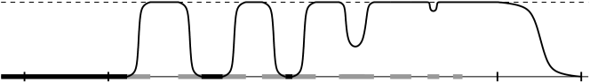
     $a_{1}$         $a+r$                                                            $b_{1}$         $b+r$

Figure 1: The graph of $f_{\varepsilon}(t,0)$. Bold black: $\Omega_{2\varepsilon}$; grey: $\Omega\setminus\Omega_{2\varepsilon}$.

Let $r>0$ be such that $B_{r}^{1}(a)\times B_{r}^{d-1}\subset\Omega$ and $B_{r}^{1}(b)\times B_{r}^{d-1}\subset{\mathbb{R}}^{d}\setminus\Omega$. Let $\varphi$ (a smoothing kernel) be a smooth non-negative function supported in the unit ball such that $\int\varphi\,dx=1$. For $\varepsilon>0$ we set $\varphi_{\varepsilon}(x)=\varphi(x/\varepsilon)/\varepsilon^{d}$, i.e. $\text{supp}(\varphi_{\varepsilon})=B_{\varepsilon}^{d}$ and $\int\varphi_{\varepsilon}\,dx=1$. Let $\Omega_{\varepsilon}=\{x\in\Omega\mid\text{dist}(x,\partial\Omega)>\varepsilon\}$ and let $h_{\varepsilon}=(1-{\bf{1}}_{\Omega_{\varepsilon}})*\varphi_{\varepsilon}$ where ${\bf{1}}_{\Omega_{\varepsilon}}$ is the characteristic function of $\Omega_{\varepsilon}$ and $*$ denotes the convolution. Let $F_{0}$ be the finitely supported function such that $\partial_{1}F_{0}(x)=\varphi_{r}(x-p)-\varphi_{r}(x-q)$ and, finally, we set $f_{\varepsilon}=F_{0}h_{\varepsilon}$ (see Figure 1).

Observe that $\Omega\cap\text{supp}(\partial_{1}f_{\varepsilon})=V\cap\text{supp}(\partial_{1}f_{\varepsilon})$ where $V=[a_{1},b_{1}]\times B_{r}^{d-1}$ with $a_{1}=a-r$ and $b_{1}=b-r$. Notice also that for any $y=(x_{2},\dots,x_{d})$ we have

$$f_{\varepsilon}(a_{1},y)=0,\qquad f_{\varepsilon}(b_{1},y)=F_{0}(b_{1},y)=\int_{{\mathbb{R}}}\varphi_{r}(t,y)\,dt,$$

and by the choice of coordinates we have $\Gamma(l_{v},f)=\partial_{1}f$. Hence

$$\int_{\Omega}\Gamma(l_{v},f_{\varepsilon})\rho\,dx =\int_{V}(\partial_{1}f_{\varepsilon})\rho\,dx=\int_{B_{r}^{d-1}}dy\int_{a_{1}}^{b_{1}}\partial_{1}f_{\varepsilon}(t,y)\rho(t,y)\,dt$$

$$=\int_{B_{r}^{d-1}}\Bigg{(}f_{\varepsilon}(b_{1},y)\rho(b_{1},y)-\int_{a_{1}}^{b_{1}}f_{\varepsilon}(t,y)\partial_{1}\rho(t,y)\,dt\Bigg{)}\,dy$$

$$=\Bigg{(}\int_{B_{r}^{d-1}}\rho(b_{1},y)\,dy\int_{{\mathbb{R}}}\varphi_{r}(t,y)\,dt\Bigg{)}-\int_{V}f_{\varepsilon}\partial_{1}\rho\,dx$$

$$\geq\min_{|y|<r}\rho(b_{1},y)-\int_{V}f_{\varepsilon}\partial_{1}\rho\,dx.$$

On the other hand, we have $0\leq f_{\varepsilon}\leq r^{-d}$, $\Omega\cap\text{supp}(f_{\varepsilon})\subset(\Omega\setminus\Omega_{2\varepsilon})\cap V$, and the Lebesgue measure of this set tends to $0$ as $\varepsilon\to 0$. Hence

$$\left|\int_{\Omega}f_{\varepsilon}\big{(}{\bf L}(l_{v})-\partial_{1}\rho\big{)}\,dx\right|\leq r^{-d}\int_{(\Omega\setminus\Omega_{2\varepsilon})\cap V}\big{|}{\bf L}(l_{v})-\partial_{1}\rho\big{|}\,dx\to 0\quad\text{as $\varepsilon\to 0$},$$

thus, setting $C=\min_{|y|<r}\rho(b_{1},y)$, we obtain

$$\int_{\Omega}\Big{(}f_{\varepsilon}{\bf L}(l_{v})+{\bf\Gamma}(f_{\varepsilon},l_{v})\Big{)}\rho\,dx\geq\int_{\Omega}f_{\varepsilon}{\bf L}(l_{v})\rho\,dx+C-\int_{\Omega}f_{\varepsilon}\partial_{1}\rho\,dx\underset{\varepsilon\to 0}{\to}C$$

which contradicts Lemma 2.9 because $C>0$.  

Remark 2.27.

The equation $\hat{\Delta}=0$ of the boundary being given, the problem of finding a symmetric matrix $(g^{ij})(x)$ formed with second degree polynomials and first degree polynomial $S^{i}$ such that

$$\sum_{j}g^{ij}\partial_{j}\hat{\Delta}=S^{i}\hat{\Delta}$$

is a linear problem in the coefficients of $g^{ij}$ and $S^{i}$ (there are $d(d+1)^{2}(d+2)/4+d(d+1)$ such coefficients) which can be easily solved for small $d$.

In the case when each $\Delta_{k}=0$ is a rational hypersurface, i.e., it can be parametrized by rational functions (this is the case in all known so far solutions of the DOP problem), it could be more convenient to compute the coefficients of the $g^{ij}$ from the boundary condition rewritten in the form

$$\sum_{j}g^{ij}\,dx_{j}^{*}=0\qquad\text{on}\qquad\{\hat{\Delta}_{k}=0\}$$

(cf. Remark 2.22). This is also a system of linear equations on the coefficients of the $g^{ij}$. For example, when $d=2$ and $x_{1}=\xi_{1}(t)$, $x_{2}=\xi_{2}(t)$ is a rational parametrization of $\Delta_{k}=0$, we need to equate to zero the coefficients of all powers of $t$ in the numerators of

$$g^{11}\dot{\xi}_{2}(t)-g^{12}\dot{\xi}_{1}(t)\qquad\text{and}\qquad g^{21}\dot{\xi}_{2}(t)-g^{22}\dot{\xi}_{1}(t).$$

Remark 2.28.

As soon as the matrix $(g^{ij})$ is known, all the admissible measure densities $\rho$ can be found as follows.The conditions (2.15) yield a system of linear equations for the unknown parameters in (2.19) (the coefficients of $Q$ and the numbers $\gamma_{q}$). Then it remains to select those solutions which satisfy the integrability conditions. In dimension $2$, if $\Omega$ and $\rho$ are given in some local curvilinear coordinates by $x^{p}>y^{2}$ and $(x^{p}-y^{2})^{\alpha}f(x,y)$ (with $f(0,0)\neq 0$) respectively, then the integrability condition reads $\alpha>-\tfrac{1}{2}-\tfrac{1}{p}$. If $\Omega$ and $\rho$ are given locally by $0<y<x^{p}$ and $y^{\alpha}(x^{p}-y)^{\beta}f(x,y)$ respectively, then it reads $\alpha+\beta>-1-\frac{1}{p}$. Note that only these singularities occur in our classification in dimension $2$.

Remark 2.29.

When the boundary equation has maximal degree $2d$, then it is proportional to the determinant of the metric $\Delta$. In this case, if $\Delta^{-1/2}$ is integrable on the domain , then the Laplace-Beltrami operator associated with the co-metric $g$ is a solution of the DOP problem on $\Omega$. It turns out that in any example where it is the case, the associated curvature (in dimension $2$ the scalar curvature) is constant, and even either $0$ either positive. Lev Soukhanov recently proved that in the general case, whenever the boundary has maximal degree $2d$, the associated metric is the product of Einstein metrics [66], and it is locally homogeneous, i. e., any two points have isometric neighbourhoods [67]. The latter fact is proven in [67] when polynomials are ordered by any weighted degree.

3 The bounded solutions in dimension 2

In this section, we concentrate on the DOP problem in dimension 2 for bounded domains. The central result of this section is the following

Theorem 3.1.

In ${\mathbb{R}}^{2}$, up to affine transformations, there are exactly 10 relatively compact sets and a one-parameter family for which there exists a solution for the DOP problem: the triangle, the square, the disk, and the areas bounded by two co-axial parabolas, by one parabola and two tangent lines, by one parabola, its axis, and a tangent line, by the nodal cubic $y^{2}=x^{2}+x^{3}$, by the cuspidal cubic $y^{2}=x^{3}$ and one tangent, by the cuspidal cubic $y^{2}=x^{3}$ and the vertical line $x=1$, by a swallow tail, or by a deltoid curve (see Section 4 for more details).

This theorem is an immediate consequence from Propositions 3.12, 3.16, 3.19, 3.20, and 3.24. Since we look at bounded domains, we may therefore reduce to the SDOP problem, and we solve the algebraic problem described in Section 2.2 in the particular case of dimension 2. For basic references on plane algebraic curves and their singularities, see [12], [28, Ch. I, §3]. [76].

In the following definition we restrict ourselves by dimension 2, but it can be obviously extended to any dimension.

Definition 3.2 (AlgDOP problem).

Let ${\mathbb{K}}$ be ${\mathbb{R}}$ or ${\mathbb{C}}$ and let $a,b,c,\hat{\Delta}$ be polynomials in ${\mathbb{K}}[x,y]$. We say that $(a,b,c,\hat{\Delta})$ is a solution of the Algebraic counterpart of the DOP problem over ${\mathbb{K}}$ ($\,{\mathbb{K}}$-AlgDOP problem for short), if $a$, $b$, and $c$ are of degree at most $2$, the polynomial $\Delta:=ac-b^{2}$ is not identically zero, and $\hat{\Delta}$ is a square-free polynomial which divides each of the following three polynomials:

$$\Delta,\qquad a\partial_{1}\hat{\Delta}+b\partial_{2}\hat{\Delta},\qquad b\partial_{1}\hat{\Delta}+c\partial_{2}\hat{\Delta}.$$

Due to Theorem 2.21, if $(\Omega,g,\rho)$ is a solution to the DOP problem and with a bounded $\Omega$, then $(g^{11},g^{12},g^{22},\hat{\Delta})$ is a solution to the ${\mathbb{R}}$-AlgDOP problem where $\hat{\Delta}=0$ is the minimal equation of $\partial\Omega$. So, our strategy is to find all solutions to the ${\mathbb{C}}$-AlgDOP problem up to affine linear transformations of ${\mathbb{C}}^{2}$, then to find all solutions to the ${\mathbb{R}}$-AlgDOP problem such that ${\mathbb{R}}^{2}\setminus\{\hat{\Delta}=0\}$ has a bounded component, and eventually to find all possible mesures $\rho$.

It is clear that the condition that $\hat{\Delta}$ divides $a\partial_{1}\hat{\Delta}+b\partial_{2}\hat{\Delta}$ and $b\partial_{1}\hat{\Delta}+c\partial_{2}\hat{\Delta}$ is equivalent to the condition that for each irreducible factor $\Delta_{1}$ of $\hat{\Delta}$ one has

$$a\partial_{1}\Delta_{1}+b\partial_{2}\Delta_{1}=L_{1}\Delta_{1}$$ (3.26)

$$b\partial_{1}\Delta_{1}+c\partial_{2}\Delta_{1}=L_{2}\Delta_{1}$$ (3.27)

where $\deg L_{i}\leq 1,i=1,2$. The equations (3.26)–(3.27), in their turn, being equivalent to

$$a(\xi,\eta)\dot{\eta}=b(\xi,\eta)\dot{\xi},\qquad b(\xi,\eta)\dot{\eta}=c(\xi,\eta)\dot{\xi}$$ (3.28)

for any local analytic branch $x=\xi(t)$, $y=\eta(t)$ of the curve $\Delta_{1}=0$ (since $\Delta_{1}$ is irreducible, the equalities (3.28) for an arbitrary local branch of $\Delta_{1}=0$ imply the same equalities for all local branches of $\Delta_{1}=0$).

The proof of Theorem 3.1 is divided in many parts. In Section 3.1, we prove that the curves $\{\hat{\Delta}=0\}$ may have flex or planar points at infinity only (Lemma 3.6), unless $\Delta$ is reducible. We also describe the various singularities which may occur at finite distance (Corollary 3.5) and the behavior at infinity (Lemma 3.7). Section 3.2 studies the case where $\Delta$ is irreducible of degree $4$, while the Sections 3.3–3.5 concentrate on the reducible case.

3.1 A preliminary study of Newton polygons of $a,b,c$ and $\Delta$

Let $(a,b,c,\hat{\Delta})$ be a solution to the ${\mathbb{C}}$-AlgDOP problem, $\Delta=ac-b^{2}$, and $\Delta_{1}$ be an irreducible factor of $\hat{\Delta}$ which is not a common factor of $a$, $b$, and $c$. Note that the last condition is always satisfied when $\Delta$ has an irreducible component of degree $\geq 3$.

We shall use projective coordinates $(X:Y:Z)$ such that $x=X/Z,y=Y/Z$ and denote $L_{\infty}$ the line $Z=0$ in ${\mathbb{CP}}^{2}$. Let $\gamma$ be an analytic branch of the curve $\Delta_{1}=0$ at some finite or infinite point, i.e. $\gamma$ is a germ at $0$ of a non-constant meromorphic mapping ${\mathbb{C}}\to{\mathbb{C}}^{2}$, $t\mapsto(\xi(t),\eta(t))$ such that $\Delta_{1}(\xi(t),\eta(t))=0$. Let $v_{\gamma}:{\mathbb{C}}[x,y]\to\mathbb{Z}\cup\{\infty\}$ be the corresponding valuation, i.e. $v_{\gamma}(f)={\rm ord\,}_{t}f\big{(}\xi(t),\eta(t)\big{)}$ where

$${\rm ord\,}_{t}u(t)=\begin{cases}n&\text{if $u(t)=\sum_{k\geq n}u_{k}t^{k}$ and $u_{n}\neq 0$,}\\ \infty&\text{if $u(t)=0$}\end{cases}$$

We denote $p=v_{\gamma}(x)={\rm ord\,}\xi$ and $q=v_{\gamma}(y)={\rm ord\,}\eta$.

Lemma 3.3.

(a) Suppose that none of $\xi(t)$, $\eta(t)$ is constant. Then

$$v_{\gamma}(a)-v_{\gamma}(b)=v_{\gamma}(b)-v_{\gamma}(c)={\rm ord\,}_{t}\dot{\xi}-{\rm ord\,}_{t}\dot{\eta}.$$ (3.29)

(b) Suppose that $\eta(t)$ is constant. Then $v_{\gamma}(b)=v_{\gamma}(c)=\infty$, i.e., $b$ and $c$ vanish identically on $\gamma$.

Proof —

(a) By (3.28), both $(a,b)$ and $(b,c)$ are proportional to $(\dot{\xi},\dot{\eta})$. Then, let us show that no one of the coefficients $a,b$ and $c$ vanishes identically along $\gamma$. Indeed if one vanishes then so will do the other ones because of this proportionality. Then $\Delta_{1}$ divides $a$, $b$, and $c$ which contradicts our assumption about $\Delta_{1}$.

Then, again by (3.28), we have

$$v_{\gamma}(a)+{\rm ord\,}\dot{\eta}=v_{\gamma}(b)+{\rm ord\,}\dot{\xi},\quad v_{\gamma}(b)+{\rm ord\,}\dot{\eta}=v_{\gamma}(c)+{\rm ord\,}\dot{\xi}.$$

(b) Straightforward from the proportionality of $(a,b)$ and $(b,c)$ to $(\dot{\xi},0)$.  

As usually, for a polynomial $u=\sum u_{kl}x^{k}y^{l}$, we define its Newton polygon ${\cal N}(u)$ as the convex hull in ${\mathbb{R}}^{2}$ of the set $\{(k,l)\,|\,u_{kl}\neq 0\}$.

Recall that $p=v_{\gamma}(x)$, $q=v_{\gamma}(y)$. We have $v_{\gamma}(x^{k}y^{l})=L_{\gamma}(k,l)$ where $L_{\gamma}$ is the linear form $L_{\gamma}(r,s)=pr+qs$. Thus, for any polynomial $u(x,y)$ we have $v_{\gamma}(u)\geq\min_{{\cal N}(u)}L_{\gamma}$ and if the minimum of $L_{\gamma}$ is attained at a single vertex of ${\cal N}(u)$, then then $v_{\gamma}(u)=\min_{{\cal N}(u)}L_{\gamma}$

The notation of the style $b=\hskip 0.0pt\left[\text{\lower 2.84526pt\hbox{\vbox to12.51918pt{\vfill\hbox{\hbox to0.0pt{\smash{\raise 9.6739pt\hbox{{{$\bullet$}}}}}\hbox to0.0pt{\smash{\raise 4.83694pt\hbox{{{$\circ$}}{{$\bullet$}}}}}{{$\bullet$}}{{$\circ$}}{{$\circ$}}}\vskip-2.27621pt}}}\right]$ (any combination of $\circ$ and $\bullet$) means that $b$ is a linear combination of monomials corresponding to the $\bullet$’s. For example, $b=\hskip 0.0pt\left[\text{\lower 2.84526pt\hbox{\vbox to12.51918pt{\vfill\hbox{\hbox to0.0pt{\smash{\raise 9.6739pt\hbox{{{$\bullet$}}}}}\hbox to0.0pt{\smash{\raise 4.83694pt\hbox{{{$\circ$}}{{$\bullet$}}}}}{{$\bullet$}}{{$\circ$}}{{$\circ$}}}\vskip-2.27621pt}}}\right]$ means that $b_{01}=b_{10}=b_{20}=0$ (the coefficients of $y$, $x$, and $x^{2}$) and the other coefficients may or may not be zero.

In the following lemma, we look for restrictions on Newton polygons of $a$, $b$, and $c$ imposed by the fact that $(\xi,\eta)$ has a given valuation $(p,q)$. The cases $p$ or $q$ negative correspond to points at infinity.

Lemma 3.4.

(a) If $(p,q)=(1,2)$, then $b=\hskip 0.0pt\left[\text{\lower 2.84526pt\hbox{\vbox to12.51918pt{\vfill\hbox{\hbox to0.0pt{\smash{\raise 9.6739pt\hbox{{{$\bullet$}}}}}\hbox to0.0pt{\smash{\raise 4.83694pt\hbox{{{$\bullet$}}{{$\bullet$}}}}}{{$\circ$}}{{$\bullet$}}{{$\bullet$}}}\vskip-2.27621pt}}}\right]$ and $c=\hskip 0.0pt\left[\text{\lower 2.84526pt\hbox{\vbox to12.51918pt{\vfill\hbox{\hbox to0.0pt{\smash{\raise 9.6739pt\hbox{{{$\bullet$}}}}}\hbox to0.0pt{\smash{\raise 4.83694pt\hbox{{{$\bullet$}}{{$\bullet$}}}}}{{$\circ$}}{{$\circ$}}{{$\bullet$}}}\vskip-2.27621pt}}}\right]$.
(b) If $(p,q)=(1,3)$, then $b=\hskip 0.0pt\left[\text{\lower 2.84526pt\hbox{\vbox to12.51918pt{\vfill\hbox{\hbox to0.0pt{\smash{\raise 9.6739pt\hbox{{{$\bullet$}}}}}\hbox to0.0pt{\smash{\raise 4.83694pt\hbox{{{$\bullet$}}{{$\bullet$}}}}}{{$\circ$}}{{$\circ$}}{{$\bullet$}}}\vskip-2.27621pt}}}\right]$ and $c=\hskip 0.0pt\left[\text{\lower 2.84526pt\hbox{\vbox to12.51918pt{\vfill\hbox{\hbox to0.0pt{\smash{\raise 9.6739pt\hbox{{{$\bullet$}}}}}\hbox to0.0pt{\smash{\raise 4.83694pt\hbox{{{$\circ$}}{{$\bullet$}}}}}{{$\circ$}}{{$\circ$}}{{$\circ$}}}\vskip-2.27621pt}}}\right]$, in particular,
${\rm mult}_{(0,0)}\Delta\geq 2$.
(c) $(p,q)=(1,4)$ is impossible.
(d) If $(p,q)=(-1,0)$, then $b=\hskip 0.0pt\left[\text{\lower 2.84526pt\hbox{\vbox to12.51918pt{\vfill\hbox{\hbox to0.0pt{\smash{\raise 9.6739pt\hbox{{{$\bullet$}}}}}\hbox to0.0pt{\smash{\raise 4.83694pt\hbox{{{$\bullet$}}{{$\bullet$}}}}}{{$\bullet$}}{{$\bullet$}}{{$\circ$}}}\vskip-2.27621pt}}}\right]$, $c=\hskip 0.0pt\left[\text{\lower 2.84526pt\hbox{\vbox to12.51918pt{\vfill\hbox{\hbox to0.0pt{\smash{\raise 9.6739pt\hbox{{{$\bullet$}}}}}\hbox to0.0pt{\smash{\raise 4.83694pt\hbox{{{$\bullet$}}{{$\bullet$}}}}}{{$\bullet$}}{{$\bullet$}}{{$\circ$}}}\vskip-2.27621pt}}}\right]$, and $c_{10}+c_{11}=0$.
(e) If $(p,q)=(-1,1)$, then $b=\hskip 0.0pt\left[\text{\lower 2.84526pt\hbox{\vbox to12.51918pt{\vfill\hbox{\hbox to0.0pt{\smash{\raise 9.6739pt\hbox{{{$\bullet$}}}}}\hbox to0.0pt{\smash{\raise 4.83694pt\hbox{{{$\bullet$}}{{$\bullet$}}}}}{{$\bullet$}}{{$\circ$}}{{$\circ$}}}\vskip-2.27621pt}}}\right]$, $c=\hskip 0.0pt\left[\text{\lower 2.84526pt\hbox{\vbox to12.51918pt{\vfill\hbox{\hbox to0.0pt{\smash{\raise 9.6739pt\hbox{{{$\bullet$}}}}}\hbox to0.0pt{\smash{\raise 4.83694pt\hbox{{{$\bullet$}}{{$\bullet$}}}}}{{$\bullet$}}{{$\circ$}}{{$\circ$}}}\vskip-2.27621pt}}}\right]$, and $c_{00}+c_{01}=0$.
(f). $p=-1$ and $2\leq q<\infty$ is impossible.
(g) If $(p,q)\in\{(-2,-1),\,(-3,-2),\,(-4,-3)\}$, then $b=\hskip 0.0pt\left[\text{\lower 2.84526pt\hbox{\vbox to12.51918pt{\vfill\hbox{\hbox to0.0pt{\smash{\raise 9.6739pt\hbox{{{$\bullet$}}}}}\hbox to0.0pt{\smash{\raise 4.83694pt\hbox{{{$\bullet$}}{{$\bullet$}}}}}{{$\bullet$}}{{$\bullet$}}{{$\circ$}}}\vskip-2.27621pt}}}\right]$ and $c=\hskip 0.0pt\left[\text{\lower 2.84526pt\hbox{\vbox to12.51918pt{\vfill\hbox{\hbox to0.0pt{\smash{\raise 9.6739pt\hbox{{{$\bullet$}}}}}\hbox to0.0pt{\smash{\raise 4.83694pt\hbox{{{$\bullet$}}{{$\circ$}}}}}{{$\bullet$}}{{$\bullet$}}{{$\circ$}}}\vskip-2.27621pt}}}\right]$.
(h) If $(p,q)=(-2,1)$, then $b=\hskip 0.0pt\left[\text{\lower 2.84526pt\hbox{\vbox to12.51918pt{\vfill\hbox{\hbox to0.0pt{\smash{\raise 9.6739pt\hbox{{{$\bullet$}}}}}\hbox to0.0pt{\smash{\raise 4.83694pt\hbox{{{$\bullet$}}{{$\bullet$}}}}}{{$\bullet$}}{{$\circ$}}{{$\circ$}}}\vskip-2.27621pt}}}\right]$ and $c=\hskip 0.0pt\left[\text{\lower 2.84526pt\hbox{\vbox to12.51918pt{\vfill\hbox{\hbox to0.0pt{\smash{\raise 9.6739pt\hbox{{{$\bullet$}}}}}\hbox to0.0pt{\smash{\raise 4.83694pt\hbox{{{$\circ$}}{{$\circ$}}}}}{{$\circ$}}{{$\circ$}}{{$\circ$}}}\vskip-2.27621pt}}}\right]$.
(i) $(p,q)=(3,4)$ is impossible.

Proof — (a) If $(p,q)=(1,2)$, then $v_{\gamma}(\dot{\xi})=0$ and $v_{\gamma}(\dot{\eta})=1$. Hence, by (3.29) we have $v_{\gamma}(b)=v_{\gamma}(a)+1\geq 1$ and $v_{\gamma}(c)=v_{\gamma}(a)+2\geq 2$ and the result follows from the fact that $v_{\gamma}(1)=0$, $v_{\gamma}(x)=1$, and $v_{\gamma}(x^{k}y^{l})\geq 2$ when $(k,l)\not\in\{(0,0),(0,1)\}$.

(b) If $(p,q)=(1,3)$, then $v_{\gamma}(\dot{\xi})=0$ and $v_{\gamma}(\dot{\eta})=2$. Hence, by (3.29) we have $v_{\gamma}(b)=v_{\gamma}(a)+2\geq 2$ and $v_{\gamma}(c)=v_{\gamma}(b)+2=v_{\gamma}(a)+4\geq 4$. The values of $v_{\gamma}$ on the monomials of degree $\leq 2$ are:

$$v_{\gamma}(1)=0,\;\;v_{\gamma}(x)=1,\;\;v_{\gamma}(x^{2})=2,\;\;v_{\gamma}(y)=3,\;\;v_{\gamma}(xy)=4,\;\;v_{\gamma}(y^{2})=6.$$ (3.30)

Thus, $v_{\gamma}(b)\geq 2$ implies $b_{00}=b_{01}=0$ and $v_{\gamma}(c)\geq 4$ implies $c_{00}=c_{10}=c_{20}=c_{01}=0$. In particular, ${\rm mult}_{(0,0)}b\geq 1$ and ${\rm mult}_{(0,0)}c\geq 2$. Hence, ${\rm mult}_{(0,0)}(b^{2}-ac)\geq 2$

(c) If $(p,q)=(1,4)$, then $v_{\gamma}(\dot{\xi})=0$ and $v_{\gamma}(\dot{\eta})=3$. Hence, by (3.29) we have

$$v_{\gamma}(c)-v_{\gamma}(b)=v_{\gamma}(b)-v_{\gamma}(a)=3$$ (3.31)

The values of $v_{\gamma}$ on the monomials of degree $\leq 2$ are:

$$v_{\gamma}(1)=0,\;\;v_{\gamma}(x)=1,\;\;v_{\gamma}(x^{2})=2,\;\;v_{\gamma}(y)=4,\;\;v_{\gamma}(xy)=5,\;\;v_{\gamma}(y^{2})=8.$$

Hence, we have $\{v_{\gamma}(a),v_{\gamma}(b),v_{\gamma}(c)\}\subset\{0,1,2,4,5,8\}$. Under this condition, (3.31) is possible only for $v_{\gamma}(a)=2$, $v_{\gamma}(b)=5$, $v_{\gamma}(c)=8$, hence $a=\hskip 0.0pt\left[\text{\lower 2.84526pt\hbox{\vbox to12.51918pt{\vfill\hbox{\hbox to0.0pt{\smash{\raise 9.6739pt\hbox{{{$\bullet$}}}}}\hbox to0.0pt{\smash{\raise 4.83694pt\hbox{{{$\bullet$}}{{$\bullet$}}}}}{{$\circ$}}{{$\circ$}}{{$\bullet$}}}\vskip-2.27621pt}}}\right]$, $b=\hskip 0.0pt\left[\text{\lower 2.84526pt\hbox{\vbox to12.51918pt{\vfill\hbox{\hbox to0.0pt{\smash{\raise 9.6739pt\hbox{{{$\bullet$}}}}}\hbox to0.0pt{\smash{\raise 4.83694pt\hbox{{{$\circ$}}{{$\bullet$}}}}}{{$\circ$}}{{$\circ$}}{{$\circ$}}}\vskip-2.27621pt}}}\right]$, and $c=\hskip 0.0pt\left[\text{\lower 2.84526pt\hbox{\vbox to12.51918pt{\vfill\hbox{\hbox to0.0pt{\smash{\raise 9.6739pt\hbox{{{$\bullet$}}}}}\hbox to0.0pt{\smash{\raise 4.83694pt\hbox{{{$\circ$}}{{$\circ$}}}}}{{$\circ$}}{{$\circ$}}{{$\circ$}}}\vskip-2.27621pt}}}\right]$. It follows that $\Delta=y^{2}f(x,y)$. This is impossible because $\gamma$ cannot be a branch of a polynomial of degree $\leq 2$.

(d) $(p,q)=(-1,0)$. If $\dot{\eta}=0$, we use Lemma 3.3(b). Otherwise the proof is similar to (a)–(c). Indeed, we have ${\rm ord\,}_{t}\dot{\xi}=-2$ and ${\rm ord\,}_{t}\dot{\eta}\geq 0$, thus $v_{\gamma}(c)-v_{\gamma}(b)=v_{\gamma}(b)-v_{\gamma}(a)\geq 2$ by (3.31). We have $v_{\gamma}(x^{k}y^{l})=-k$, thus $v_{\gamma}(a)\geq-2$, hence $v_{\gamma}(c)>v_{\gamma}(b)=v_{\gamma}(a)+2\geq 0$. Therefore $b_{20}=c_{20}=0$ (otherwise $v_{\gamma}(b)$ or $v_{\gamma}(c)$ would be $-2$) and $b_{10}+b_{11}=c_{10}+c_{11}=0$ (otherwise $v_{\gamma}(b)$ or $v_{\gamma}(c)$ would be $-1$).

(e) If $(p,q)=(-1,1)$, then by (3.29) we have $v_{\gamma}(c)-v_{\gamma}(b)=v_{\gamma}(b)-v_{\gamma}(a)=2$, hence $v_{\gamma}(a)\geq-2$, $v_{\gamma}(b)\geq 0$, $v_{\gamma}(c)\geq 2$ and the result follows (as in point (d), $c_{00}+c_{11}=0$ because otherwise we would have $v_{\gamma}(c)=0$).

(f) We have $v_{\gamma}(c)-v_{\gamma}(b)=v_{\gamma}(b)-v_{\gamma}(a)=q+1$ and $v_{\gamma}(x^{2},x,1,xy,y,y^{2})=(-2,-1,0,q-1,q,2q)$. Thus, $v_{\gamma}(a,b,c)=(-2,q-1,2q)$, i.e. $b=\hskip 0.0pt\left[\text{\lower 2.84526pt\hbox{\vbox to12.51918pt{\vfill\hbox{\hbox to0.0pt{\smash{\raise 9.6739pt\hbox{{{$\bullet$}}}}}\hbox to0.0pt{\smash{\raise 4.83694pt\hbox{{{$\bullet$}}{{$\bullet$}}}}}{{$\circ$}}{{$\circ$}}{{$\circ$}}}\vskip-2.27621pt}}}\right]$ and $c=\hskip 0.0pt\left[\text{\lower 2.84526pt\hbox{\vbox to12.51918pt{\vfill\hbox{\hbox to0.0pt{\smash{\raise 9.6739pt\hbox{{{$\bullet$}}}}}\hbox to0.0pt{\smash{\raise 4.83694pt\hbox{{{$\circ$}}{{$\circ$}}}}}{{$\circ$}}{{$\circ$}}{{$\circ$}}}\vskip-2.27621pt}}}\right]$, Therefore, $\Delta=y^{2}f(x,y)$. This is impossible because $\gamma$ cannot be a branch of a polynomial of degree $\leq 2$.

(g,h) The proof is similar to the previous cases.

(i) We have $v_{\gamma}\{a,b,c\}\subset v_{\gamma}\{1,x,y,x^{2},xy,y^{2}\}=\{0,3,4,6,7,8\}$. Combining this with $v_{\gamma}(c)-v_{\gamma}(b)=v_{\gamma}(b)-v_{\gamma}(a)={\rm ord\,}_{t}\dot{\eta}-{\rm ord\,}_{t}\dot{\xi}=3-2=1$, we obtain $v_{\gamma}(a)=6$, $v_{\gamma}(b)=7$, $v_{\gamma}(c)=8$, i.e. $a=\hskip 0.0pt\left[\text{\lower 2.84526pt\hbox{\vbox to12.51918pt{\vfill\hbox{\hbox to0.0pt{\smash{\raise 9.6739pt\hbox{{{$\bullet$}}}}}\hbox to0.0pt{\smash{\raise 4.83694pt\hbox{{{$\circ$}}{{$\bullet$}}}}}{{$\circ$}}{{$\circ$}}{{$\bullet$}}}\vskip-2.27621pt}}}\right]$, $b=\hskip 0.0pt\left[\text{\lower 2.84526pt\hbox{\vbox to12.51918pt{\vfill\hbox{\hbox to0.0pt{\smash{\raise 9.6739pt\hbox{{{$\bullet$}}}}}\hbox to0.0pt{\smash{\raise 4.83694pt\hbox{{{$\circ$}}{{$\bullet$}}}}}{{$\circ$}}{{$\circ$}}{{$\circ$}}}\vskip-2.27621pt}}}\right]$, $c=\hskip 0.0pt\left[\text{\lower 2.84526pt\hbox{\vbox to12.51918pt{\vfill\hbox{\hbox to0.0pt{\smash{\raise 9.6739pt\hbox{{{$\bullet$}}}}}\hbox to0.0pt{\smash{\raise 4.83694pt\hbox{{{$\circ$}}{{$\circ$}}}}}{{$\circ$}}{{$\circ$}}{{$\circ$}}}\vskip-2.27621pt}}}\right]$. Thus, ${\rm mult}_{0}(\Delta)=4$, i.e., $\Delta=0$ is a union of four lines which contradicts the condition $(p,q)=(3,4)$.  

According to the standard terminology (see, e.g. [28, Ch. I, §2.4]), we say that an analytic branch $\beta$ of an algebraic curve in ${\mathbb{CP}}^{2}$ is generic, flex, planar, or has singularity of type $A_{2}$ (called also cusp) or $E_{6}$ if there exists an affine coordinate chart $(u,v)$ such that the pair $(p,q):=v_{\gamma}(u,v)$ is as in the second column of Table 1 in Section 3.2.

Corollary 3.5.

(a). $\Delta$ cannot have a singularity of type $E_{6}$ at a finite point.
(b). Suppose that $\gamma$ is a singular branch of $\Delta_{1}$ of type $A_{2}$ at a point $P\in L_{\infty}$ and $L_{\infty}$ is not tangent to $\gamma$ at $P$. Then there is another branch of $\Delta$ at $P$, or $\deg\Delta=3$.

Proof —

The point (a) follows from Lemma 3.4(i).

Point (b) corresponds to $(p,q)=(-2,1)$ for a suitable choice of the coordinates (whereas $(-3,-1)$ corresponds to a cusp on $L_{\infty}$ tangent to $L_{\infty}$). We are therefore in case Lemma 3.4(h). Hence $b(x,0)=b_{00}$ (a constant) and $c(x,0)=0$ whence $\Delta(x,0)=b_{00}^{2}$. This means that the local intersection of the line $\{y=0\}$ with $\{\Delta=0\}$ at $P$ is equal to $\deg\Delta$. On the other hand, the local intersection of this line with $\gamma$ at $P$ is $3$, thus either $\Delta$ has another branch at $P$ or $\deg\Delta=3$.  

Lemma 3.6.

Let $\gamma$ be a flex or planar branch of $\Delta_{1}$ at $P$. Then
(a) if $P\in L_{\infty}$, then $\gamma$ is tangent to $L_{\infty}$.
(b) if $P\not\in L_{\infty}$, then $\gamma$ is not planar and ${\rm mult}_{P}(\Delta)>{\rm mult}_{P}(\hat{\Delta})$, in particular, this is impossible when $\Delta$ is irreducible.

Proof — (a) Follows from Lemma 3.4(f).

(b) The fact that $\gamma$ is not planar follows from Lemma 3.4(c). Let us choose affine coordinates so that $P$ is the origin and the axis $y=0$ is tangent to $\gamma$. Thus, ${\rm ord\,}_{t}\gamma=(1,3)$. By Lemma 3.4(b), we have ${\rm mult}_{(0,0)}\Delta\geq 2$, i.e., there is another branch $\beta$ of $\Delta$ passing through the origin. Since $\deg_{x}\Delta(x,0)\leq 4$ the multiplicities of the intersection of the axis $y=0$ with $\gamma$ and $\beta$ are $3$ (i.e., $q=3$) and $1$ respectively.

It remains to prove that $\beta$ cannot be a branch of $\hat{\Delta}$. Suppose it is. Let us choose coordinates so that the axis $x=0$ is tangent to $\beta$. Then Lemmas 3.3(b) and 3.4(a,b) applied to $\beta$ imply

$$a_{00}=a_{01}=0.$$ (3.32)

(we swap $x\leftrightarrow y$ and $a\leftrightarrow c$ in Lemma 3.4). Hence, $v_{\gamma}(a)\geq 1$. By (3.29), we have

$$v_{\gamma}(c)-v_{\gamma}(b)=v_{\gamma}(b)-v_{\gamma}(a)=2$$ (3.33)

(see the proof of Lemma 3.4(b)). Recall that the values of $v_{\gamma}$ on monomials are given by (3.30). Hence, $\{v_{\gamma}(a),v_{\gamma}(b),v_{\gamma}(c)\}\subset\{0,1,2,3,4,6\}$. Combining this with (3.33) and $v_{\gamma}(a)\geq 1$, we obtain $v_{\gamma}(a)=2$, $v_{\gamma}(b)=4$, $v_{\gamma}(c)=6$. By (3.32), this implies ${\rm mult}_{(0,0)}(a)={\rm mult}_{(0,0)}(b)={\rm mult}_{(0,0)}(c)=2$, hence ${\rm mult}_{(0,0)}(\Delta)=4$. This means that $\Delta$ is a union of four lines passing through the origin. Contradiction.  

Lemma 3.7.

Let $\gamma$ be a smooth branch of $\Delta_{1}$ at $P\in L_{\infty}$. Suppose that there exists a line $L$ passing through $P$ which is tangent to a branch $\beta$ of $\hat{\Delta}$ at a finite point $Q$. Suppose also that $\beta,\gamma\not\subset L$. Then
(a) $\beta$ is smooth at $Q$.
(b) ${\rm mult}_{P}(\Delta)\geq 2$ or $\deg\Delta\leq 3$.

Proof — Let us choose coordinates so that $L$ is the axis $y=0$ and and $\beta$ is tangent to $L$ at the origin. Then all possibilities for $\gamma$ are covered by Lemma 3.4(d)–(g) and in all these cases we have $b,c=\hskip 0.0pt\left[\text{\lower 2.84526pt\hbox{\vbox to12.51918pt{\vfill\hbox{\hbox to0.0pt{\smash{\raise 9.6739pt\hbox{{{$\bullet$}}}}}\hbox to0.0pt{\smash{\raise 4.83694pt\hbox{{{$\bullet$}}{{$\bullet$}}}}}{{$\bullet$}}{{$\bullet$}}{{$\circ$}}}\vskip-2.27621pt}}}\right]$, i.e., $b_{20}=c_{20}=0$.

(a) Let $\beta=(\xi,\eta)$ and $(p,q)={\rm ord\,}_{t}(\xi,\eta)$. Suppose that $\beta$ is singular. Then $\min(p,q)\geq 2$. We have also $q>p$ (because $L$ is tangent to $\beta$) and $q=(L.\beta)\leq 3$ (because $(L.\beta)+(L.\gamma)\leq 4$). Thus, $(p,q)=(2,3)$ hence, by (3.29), we have $v_{\beta}(c)-v_{\beta}(b)=v_{\beta}(b)-v_{\beta}(a)=1$. Combining this fact with $v_{\beta}(1,x,y,x^{2},xy,y^{2})=(0,2,3,4,5,6)$ and $b_{20}=c_{20}=0$, we obtain $v_{\beta}(a,b,c)=(4,5,6)$, i.e., $a=\hskip 0.0pt\left[\text{\lower 2.84526pt\hbox{\vbox to12.51918pt{\vfill\hbox{\hbox to0.0pt{\smash{\raise 9.6739pt\hbox{{{$\bullet$}}}}}\hbox to0.0pt{\smash{\raise 4.83694pt\hbox{{{$\circ$}}{{$\bullet$}}}}}{{$\circ$}}{{$\circ$}}{{$\bullet$}}}\vskip-2.27621pt}}}\right]$, $b=\hskip 0.0pt\left[\text{\lower 2.84526pt\hbox{\vbox to12.51918pt{\vfill\hbox{\hbox to0.0pt{\smash{\raise 9.6739pt\hbox{{{$\bullet$}}}}}\hbox to0.0pt{\smash{\raise 4.83694pt\hbox{{{$\circ$}}{{$\bullet$}}}}}{{$\circ$}}{{$\circ$}}{{$\circ$}}}\vskip-2.27621pt}}}\right]$, $c=\hskip 0.0pt\left[\text{\lower 2.84526pt\hbox{\vbox to12.51918pt{\vfill\hbox{\hbox to0.0pt{\smash{\raise 9.6739pt\hbox{{{$\bullet$}}}}}\hbox to0.0pt{\smash{\raise 4.83694pt\hbox{{{$\circ$}}{{$\circ$}}}}}{{$\circ$}}{{$\circ$}}{{$\circ$}}}\vskip-2.27621pt}}}\right]$. Thus, $\Delta$ is homogeneous. A contradiction.

(b) Combining $b_{20}=c_{20}=0$ with Lemma 3.4(a) applied to $\beta$, we obtain $b=\hskip 0.0pt\left[\text{\lower 2.84526pt\hbox{\vbox to12.51918pt{\vfill\hbox{\hbox to0.0pt{\smash{\raise 9.6739pt\hbox{{{$\bullet$}}}}}\hbox to0.0pt{\smash{\raise 4.83694pt\hbox{{{$\bullet$}}{{$\bullet$}}}}}{{$\circ$}}{{$\bullet$}}{{$\circ$}}}\vskip-2.27621pt}}}\right]$, $c=\hskip 0.0pt\left[\text{\lower 2.84526pt\hbox{\vbox to12.51918pt{\vfill\hbox{\hbox to0.0pt{\smash{\raise 9.6739pt\hbox{{{$\bullet$}}}}}\hbox to0.0pt{\smash{\raise 4.83694pt\hbox{{{$\bullet$}}{{$\bullet$}}}}}{{$\circ$}}{{$\circ$}}{{$\circ$}}}\vskip-2.27621pt}}}\right]$. Thus, it is enough to show that $c_{11}=0$. Indeed, if $\gamma$ is tangent to $L_{\infty}$, this is already proven in Lemma 3.4(g). Otherwise by Lemma 3.4(d,e,f) we have $c_{00}+c_{11}=0$ or $c_{10}+c_{11}=0$ and we know that $c_{00}=c_{10}=0$.  

3.2 The duals of quartic curves

Let $C$ be an irreducible algebraic curve in $\mathbb{P}^{2}$ of degree $d\geq 2$. Let $\check{C}$ be the dual curve in $\check{\mathbb{P}}^{2}$ is the set of all lines in ${\mathbb{P}}^{2}$ endowed with the natural structure of the projective plane, and $\check{C}$ is the set of all lines in ${\mathbb{P}}^{2}$ which are tangent to $C$.

If $t\to\gamma(t)$ is a local analytic branch of $C$, then we denote the dual branch of $\check{C}$ by $\check{\gamma}$. It is defined by $t\mapsto\check{\gamma}(t)$ where $\check{\gamma}(t)$ is the line which is tangent to $C$ at $\gamma(t)$.

Let $\gamma$ be a local branch of $C$. Let us choose affine coordinates $(X,Y)$ so that $\gamma$ is given by $X=\xi(t)$, $Y=\eta(t)$, $\xi(0)=\eta(0)=0$. Then the equation of the line $\check{\gamma}(t)$ is $(X-\xi)\dot{\eta}-(Y-\eta)\dot{\xi}=0$. Thus, in the standard homogeneous coordinates on $\check{\mathbb{P}}^{2}$ corresponding to the coordinate chart $(X,Y)$, the dual branch $\check{\gamma}$ has a parametrization of the form

$$t\mapsto(\dot{\eta}\,:\,-\dot{\xi}\,:\,\dot{\xi}\eta-\xi\dot{\eta})$$ (3.34)

and we obtain the following fact.

Lemma 3.8.

Let $\gamma$ be a local branch of $C$ and $\check{\gamma}$ the dual branch of $\check{C}$. Let $(X,Y)$ be an affine chart such that $\gamma$ has the form $X=\xi(t)$, $Y=\eta(t)$ with $0<p<q$ where $p={\rm ord\,}_{t}\xi$ and $q={\rm ord\,}_{t}\eta$. Then, in suitable affine coordinates $(\check{X},\check{Y})$ on $\check{\mathbb{P}}^{2}$, the branch $\check{\gamma}$ has the form $\check{X}=\check{\xi}(t)$, $\check{Y}=\check{\eta}(t)$ with ${\rm ord\,}_{t}\check{\xi}=q-p$ and ${\rm ord\,}_{t}\check{\eta}=q$.

For a point $P\in C$, we denote the delta-invariant of $(C,P)$ by $\delta_{P}$ or $\delta_{P}(C)$ (see [28, p. 206]). Informally speaking, $\delta_{P}$ is the number of double points of $C$ concentrated in $P$. We have (see [58, Thm. 10.2] or [28, Ch. I, Prop. 3.34])

$$2\delta_{P}=\mu+r-1=\sum m_{i}(m_{i}-1)$$

where $\mu$ is the Milnor number and $r$ is the number of local branches of $C$ at $P$, and $\mathbf{m}=[m_{1},m_{2},\dots]$ is the sequence of the multiplicities of all infinitely near points of $P$. If $P$ is a non-singular point of $C$, then $\delta_{P}=0$. It easily follows from the definition (see also [28, Ch. I, Lem. 3.32]) that

$$\delta_{P}=\delta_{P}^{0}+\sum_{i=1}^{r}\delta(\gamma_{i})\qquad\text{where}\quad\delta_{P}^{0}=\sum_{1\leq i<j\leq r}(\gamma_{i}\cdot\gamma_{j}),$$ (3.35)

$\gamma_{1},\dots,\gamma_{r}$ are local branches of $C$ at $P$, and $(\gamma_{i}\cdot\gamma_{j})$ is the intersection number of $\gamma_{i}$ and $\gamma_{j}$ at $P$.

Let $g$ be the genus of $C$. By the genus formula (see [12, p. 624, Thm. 7] or [58, §10, Eq. (1)]), we have

$$2g+2\sum_{P\in C}\delta_{P}=(d-1)(d-2).$$ (3.36)

Combining (3.35) and (3.36), we obtain

$$2g+2n+2\sum_{\gamma}\delta(\gamma)=(d-1)(d-2)$$ (3.37)

where $\gamma$ runs over all local branches of $C$ at all points and $n=\sum_{P\in C}\delta^{0}_{P}$ (only a finite number of terms in the both sums are non-zero).

For a local branch $\gamma$ of a curve $C$ at a point $P$, we denote the multiplicity of $\gamma$ at $P$ by $m(\gamma)$. If $\gamma$ is parametrized by $X=\xi(t)$, $Y=\eta(t)$ in some local coordinates $X,Y$, then $m(\gamma)=\min({\rm ord\,}_{t}\xi,{\rm ord\,}_{t}\eta)$. We set also $\varepsilon(\gamma)=2\delta(\gamma)+m(\gamma)-1$. Let $\check{d}$ be the degree of $\check{C}$. In this notation, the first Plücker formula (the class formula) takes the form (see [52, Thm. 1.3])

$$\check{d}=d(d-1)-2n-\sum_{\gamma}\varepsilon(\gamma)$$ (3.38)

and the second Plücker formula (the Riemann-Hurwitz formula for a generic projection of $\check{C}$ onto a line) is

$$2-2g=2\check{d}-d-\sum_{\gamma}(m(\check{\gamma})-1).$$ (3.39)

In the both formulas $\gamma$ runs over all local branches of $C$.

If $d=4$, then $\sum\delta(\gamma)\leq 3$ by (3.37) which is possible for the sequences of multiplicities $[2]$, $[2,2]$, $[2,2,2]$, and $[3]$ only, hence all singular branches are of the types $A_{2}$, $A_{4}$, $A_{6}$ and $E_{6}$ (recall that $A_{k}$ and $E_{6}$ are given by $v^{2}=u^{k+1}$ and $v^{3}=u^{4}$ is suitable curvilinear local coordinates). In Table 1, we list all types of local branches $\gamma(t)=(\xi(t),\eta(t))$, ${\rm ord\,}_{t}\xi=p$, ${\rm ord\,}_{t}\eta=q$, $p<q$, and their invariants contributing to (3.37), (3.38), and (3.39) (we use Lemma 3.8 to compute $\check{p}={\rm ord\,}_{t}\check{\xi}$ and $\check{q}={\rm ord\,}_{t}\check{\eta}$).

Table 1     

  $\mathbf{m}$ $(p,q)$ $(\check{p},\check{q})$ $\delta(\gamma)$ $\varepsilon(\gamma)$ $m(\check{\gamma})-1$

 

generic point - (1,2) (1,2) 0 0 0

flex point - (1,3) (2,3) 0 0 1

planar point - (1,4) (3,4) 0 0 2

$A_{2}$ [2] (2,3) (1,3) 1 3 0

$A_{4}$ [2,2] (2,4) (2,4) 2 5 1

$A_{6}$ [2,2,2] (2,4) (2,4) 3 7 1

$E_{6}$ [3] (3,4) (1,4) 3 8 0  

Thus, denoting the number of branches of the respective types by $f$ (flex), $p$ (planar), $a_{2}$, $a_{4}$, $a_{6}$, and $e_{6}$, we rewrite (3.37) – (3.39) as

$$\begin{matrix}g+n+a_{2}+2a_{4}+3a_{6}+3e_{6}=3,\\ \check{d}=12-2n-3a_{2}-5a_{4}-7a_{6}-8e_{6},\\ 2-2g=2\check{d}-4-f-2p-a_{4}-a_{6}.\end{matrix}$$

Eliminating $g$ and $\check{d}$, we obtain

$$f+2p=24-8a_{2}-15a_{4}-21a_{6}-22e_{6}-6n.$$ (3.40)

Since all the ingredients (including $g$) are non-negative, we obtain the following fact.

Lemma 3.9.

Suppose that $C$ is an irreducible quartic curve in ${\mathbb{P}}^{2}$ which has at most one smooth non-generic (i.e., flex or planar) local branch. Then $C$ is rational (i.e., $g=0$) and one of the following cases occurs:

• $(i)$ (tricuspidal quartic) $C$ has three singular points of type $A_{2}$ and no smooth non-generic branches (i.e., $f=p=0$). The dual curve $\check{C}$ is a nodal cubic.

• $(ii)$ (swallow tail) $C$ has two singular points of type $A_{2}$ and one planar point, and one ordinary double point (i.e., $f=0$, $p=n=1$). The degree of $\check{C}$ is $4$, it has one singular point of type $E_{6}$ and two flex points. The equation of $\check{C}$ in suitable affine coordinates is $y=x^{4}-x^{2}$.

• $(iii)$ Each of $C$ and $\check{C}$ has two singular points of types $A_{2}$ and $A_{4}$ and one flex point (i.e., $f=1$, $p=0$), the degree of $\check{C}$ is $4$,

• $(iv)$ Each of $C$ and $\check{C}$ has one singular point of type $E_{6}$ and one planar point (i.e., $f=0$, $p=1$). The degree of $\check{C}$ is $4$. The equation of $\check{C}$ in suitable affine coordinates is $y=x^{4}$.

In each of the cases $(i)$–$(iv)$ the formulated conditions uniquely determine the curve $C$ up to automorphism of ${\mathbb{CP}}^{2}$.

Proof —

By (3.37) we have $g+n+a_{2}+2a_{4}+3a_{6}+3e_{6}=3$. Substituting each nonnegative solution of this equation into (3.40), we see that the only cases when $f+p\leq 1$ are:

$$(i)~{}\;\;\check{d}=3,\;a_{2}=3;\qquad\qquad\quad (iii)\;\;\check{d}=4,\;a_{2}=a_{4}=1,\;f=1,$$

$$(ii)~{}\;\;\check{d}=4,\;a_{2}=2,\;p=n=1, (iv)\;\;\check{d}=4,\;e_{6}=p=1.$$

Let us show that these cases are uniquely realizable. In cases $(ii)$ and $(iv)$ this follows from the fact that $\check{C}$ has the singularity $E_{6}$, hence it has the equation $y=f(x)$, $\deg_{x}f=4$, in suitable coordinates. By affine changes of coordinates, this equation reduces to $y=x^{4}$ or $y=x^{4}-x^{2}$.

In case $(i)$, the dual curve is a nodal cubic. It is unique up to projective transformation, thus $C$ is also unique.

In case $(iii)$, let us choose homogeneous coordinates $(X:Y:Z)$ so that $A_{2}$ and $A_{4}$ are at $(0:0:1)$ and $(0:1:0)$ respectively and the lines $Y=0$ and $Z=0$ are tangent to $C$ at these points. (These are two distinct lines. Indeed, the local intersection of $C$ with the tangent lines at $A_{2}$ and $A_{4}$ is is $3$ and $4$ respectively, thus it cannot be a single line by Bezout’s theorem.) Let $F(X,Y,Z)=0$ be the equation of $C$. Let us consider the Newton polygon of the polynomial $F(X,Y,1)$. The choice of the coordinates near $A_{2}$ ensures that it is placed above the segment $[(0,2),(3,0)]$. The choice of the coordinates near $A_{4}$ ensures that the segment $[(0,2),(4,0)]$ is an edge of the Newton polygon. Hence $F=u_{30}X^{3}Z+G$ where $G=u_{40}X^{4}+u_{21}X^{2}YZ+u_{02}Y^{2}Z^{2}$. Moreover, the fact that $F$ has a single branch at $(0:1:0)$ implies that $G$ is a complete square. Hence, rescaling the coordinate, we can obtain $u_{30}=u_{40}=u_{02}=1$, $u_{11}=2$, whence the uniqueness up to projective change of coordinates.

 

Corollary 3.10.

Suppose that $C$ is an irreducible quartic curve in ${\mathbb{C}}^{2}$ which satisfies the restrictions imposed by Lemmas 3.4(h,i), 3.6 and 3.7, i.e.:

• any smooth non-generic branch of $C$ is tangent to the infinite line $L_{\infty}$;

• if $C$ meets $L_{\infty}$ transversally at a point $P$ and $C$ is smooth at $P$, then there is no line through $P$ (except, maybe, $L_{\infty}$) which is tangent to $C$ at a smooth or singular point;

• if $C$ has a cusp $A_{2}$ at a point $P\in L_{\infty}$, and $L_{\infty}$ is not the tangent to $C$ at $P$, then $C$ has another branch through $P$;

• $C$ does not have a singularity of type $E_{6}$ at a finite point.

Then one of the cases $(i)$ or $(ii)$ of Lemma 3.9 occurs and the position of $C$ with respect to the infinite line $L_{\infty}$ is one of:

• $(i_{1})$ (deltoid or $(1,3)$-hypocycloid) $L_{\infty}$ is the bitangent of $C$.

• $(i_{2})$ $L_{\infty}$ is the tangent at a cusp.

• $(ii)$ (swallow tail) $L_{\infty}$ is the tangent at the planar point.

In each of the cases $(i_{1})$ and $(ii)$ the affine curve $C$ is unique up to affine transformation of ${\mathbb{C}}^{2}$. In suitable affine coordinates, $C$ is parametrized by

• $(i_{1})$ $x=2\cos\theta+\cos 2\theta$, $y=2\sin\theta-\sin 2\theta$;

• $(i_{2})$ $x=t^{3}-2t+t^{-1}$, $y=3t-t^{-1}$;

• $(ii)$ $x=2t(2t^{2}-1)$, $y=t^{2}(3t^{2}-1)$.

Figure 2: The real quartic with $A_{2}$ and $A_{4}$

Proof — Since $\deg C=4$, there is no room for more than one non-generic tangency with $L_{\infty}$. Thus one of the cases $(i)$–$(iv)$ of Lemma 3.9 occurs. We consider them separately.

$(i)$ Let $P$ be a smooth point of $C$. Riemann-Hurwitz formula for the projection from $P$ implies that there exists a unique line $L_{P}$ through $P$ tangent to $C$ at another (smooth or singular) point.

Suppose that $(i_{2})$ does not hold. Then by Corollary 3.5(b) all infinite points of $C$ are smooth. Let $P$ be one of them. Let $Q$ be the point where $L_{P}$ is tangent to $C$. Lemma 3.7 implies $L_{P}=L_{\infty}$, i.e., $Q\in L_{\infty}$. Then, again by Lemma 3.7, we have $L_{Q}=L_{\infty}$, thus $(i_{1})$ takes place.

In Case $(i_{2})$, there are three cusps. However different choices of the one tangent to $L_{\infty}$ lead to the same result because the cusps are interchangeable by a projective automorphism of ${\mathbb{CP}}^{2}$ (one can see it, e.g., from the trigonometric parametrization).

$(ii)$ No other choice for $L_{\infty}$.

$(iii)$ Let $P$ be the flex point. Then $L_{\infty}$ is tangent to $C$ at $P$ by Lemma 3.6. Applying Riemann-Hurwitz formula to the projection from $P$, we see that there exists a line $L$ through $P$ which is tangent to $C$ at a smooth point. Contradiction with Lemma 3.7.

Remark. The existence of such $L$ can be also derived from the uniqueness of $C$ up to projective transformations. Indeed, we can realize $C$ as a real curve in ${\mathbb{R}}^{2}$ obtained by a small perturbation of a double circle: $(x^{2}+y^{2})^{2}=\varepsilon y^{3}(x+1)$, $0<\varepsilon\ll 1$. Then $L$ is clearly visible in Figure 2.

$(iv)$ Impossible by Lemma 3.6 and Lemma 3.5(a).  

Thus there are only three candidates for solutions of the ${\mathbb{C}}$-AlgDOP problem. It remains to check that the linear equations for the metric (see Remark 2.27) have non-zero solutions, and then to select the real forms corresponding to bounded domains.

Proposition 3.11.

Up to affine transformations of ${\mathbb{C}}^{2}$ and rescaling of $(a,b,c)$, there are exactly three solutions to the ${\mathbb{C}}$-AlgDOP problem under condition that $\hat{\Delta}$ is irreducible of degree $4$. The curve $C=\{\hat{\Delta}=0\}$ is as in Corollary 3.10. In Cases $(i_{1})$ and $(ii)$ the formulas for $(a,b,c)$ are given in Sections 4.11 and 4.12 respectively. In Case $(i_{2})$, $a=9x^{2}+8xy$, $b=2y^{2}+3xy-8$, $c=y^{2}-12$.

Proposition 3.12.

Up to affine transformations of ${\mathbb{R}}^{2}$ and rescaling of $(a,b,c)$, there are exactly six solutions to the ${\mathbb{R}}$-AlgDOP problem under condition that $\hat{\Delta}$ is irreducible of degree $4$: the three solutions given in Proposition 3.11 and those obtained from them by the change of coordinates $(x,y)\mapsto(ix,y)$. Only two among these solutions (those discussed in Sections 4.11 and 4.12) correspond to bounded domains in ${\mathbb{R}}^{2}$ and thus provide a solution to the DOP problem.

Proof — First let us show that each projective curve $(i)$ and $(ii)$ of Lemma 3.10 has two real forms. It is easier to check this fact for the dual curves. Indeed, for the nodal cubic (Case $(i)$) these are $y^{2}=x^{3}\pm x$, and in Case $(ii)$ these are $y=x^{4}\pm x^{2}$.

The choice of the line at infinity is unique in all the six cases. Indeed, for $(i_{1})$ and $(ii)$ it is unique even over ${\mathbb{C}}$. In Case $(i_{2})$ the curve $C$ has one or three real cusps, and if it has three cusps, they are interchangeable by an automorphism of ${\mathbb{RP}}^{2}$. Let us show that $\{\hat{\Delta}\neq 0\}$ does not have bounded components except the two cases.

$(i)$ If $C$ has three real cusps, it looks as shown in Section 4.12. So, it is clear that a tangent at a cusp is adjacent to each component of the complement of $C$. If $C$ has one real cusp, it can be realized as the $(1,1)$-hypercycloid $x=2\cos\theta+\cos 2\theta$, $y=2\sin\theta+\sin 2\theta$ in some affine chart (see Figure 3). So, in both cases $(i_{1})$ and $(i_{2})$, the line $L_{\infty}$ meets the closure of each component of the complement of $C$.

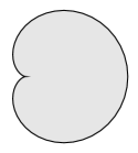
Figure 3: $(1,1)$-hypercycloid: an irrelevant solution to AlgDOP problem

$(ii)$. If $\check{C}$ is $y=x^{4}+x^{2}$, it is convex in some affine chart, hence so is $C$. Since $L_{\infty}$ is tangent to $C$, the affine part of $C$ is homeomorphic to a line dividing ${\mathbb{R}}^{2}$ into two unbounded components.

 

3.3 Cubic factor of $\hat{\Delta}$

In this section we suppose that $\Delta=\Delta_{3}\Delta_{1}$ where $\Delta_{3}$ is an irreducible cubic factor of $\hat{\Delta}$ (As above, $(a,b,c,\hat{\Delta})$ is a solution to the ${\mathbb{C}}$-AlgDOP problem $\Delta=ac-b^{2}$). By the genus formula (3.37), an irreducible cubic curve in ${\mathbb{CP}}^{2}$ is either smooth of genus one (and then depends of one parameter up to projective transformations), or rational with a single singularity of type $A_{1}$ (node) or $A_{2}$ (cusp). In the latter case the curve is projectively rigid.

Let $C$ be the quartic curve defined by $\Delta=0$ and let $C_{3}$ and $C_{1}$ be the respective irreducible components of $C$ (if $\deg\Delta=3$, then $C_{1}=L_{\infty}$).

Lemma 3.13.

$C_{3}$ is rational.

Proof — Otherwise $C_{3}$ has nine flex points. They cannot all be on $C_{1}\cup L_{\infty}$. So, this contradicts to Lemma 3.6.  

By an isomorphism of ${\mathbb{CP}}^{2}$, any rational cubic can by identified either with the nodal cubic $y^{2}=x^{3}-x^{2}$ or with the cuspidal cubic $y^{2}=x^{3}$. The nodal cubic has three flex points lying on the same line and interchangeable by automorphisms of ${\mathbb{CP}}^{2}$. The cuspidal cubic has a single flex point.

Lemma 3.14.

Suppose that $C_{3}$ is a nodal cubic. Then $\hat{\Delta}=\Delta_{3}$, the line $L_{\infty}$ is tangent to $C_{3}$ at a flex point, and $C_{1}$ is the line passing through all the three flex points of $C_{3}$.

Proof — Let $L_{0}$ be the line passing through all the flex points of $C_{3}$. Then $L_{0}\neq L_{\infty}$ by Lemma 3.6(a). Thus, at least two flex points are not on $L_{\infty}$, hence Lemma 3.6(b) implies that a non-trivial component of $\Delta/\hat{\Delta}$ passes through them. Hence, $C_{1}=L_{0}$. and $\hat{\Delta}=\Delta_{3}$.

Suppose that $C_{3}$ has more than one point at infinity. Then there is a point $P$ such that $(C_{3}.L_{\infty})_{P}=1$. Then $P$ is not a flex point by Lemma 3.6. Hence, Riemann-Hurwitz formula for the projection from $P$ implies that there exists a line $L$ through $P$ which is tangent to $C$ at some other point $Q$. If $Q$ were finite, then Lemma 3.7(b) would imply that $C_{1}$ passes through $P$. This is impossible by Bezout’s theorem because $C_{1}$ has already three intersections with $C_{3}$ at the flex points. Thus, $Q\in L_{\infty}$. Applying the same arguments to $Q$, we obtain a contradiction.

Thus, $C_{3}$ has a single point $P$ at the infinity. It remains to show that $P$ is not the node of $C_{3}$. Suppose it is. Choose coordinates $(X:Y:Z)$, $x=X/Z$,$y=Y/Z$, so that $P=(1:0:0)$, the axis $X=0$ is the tangent at a flex point, and the tangents at $P$ are $L_{\infty}$ and the axis $Y=0$. Then, up to rescaling of the coordinates, $C_{3}$ admits a parametrization $x=\xi(t)=(t-1)^{3}/t$, $y=\eta(t)=t$.

So, we have an explicit parametric equation of a component of $\hat{\Delta}$. As we pointed out in Remark 2.27, then we have a system of linear equations on the coefficients of $(a,b,c)$. The rest of the proof is just checking by hand that this system does not have any nonzero solution.

Applying Lemma 3.4(e,g) to the branches of $C_{3}$ at $P$, we obtain $b=\hskip 0.0pt\left[\text{\lower 2.84526pt\hbox{\vbox to12.51918pt{\vfill\hbox{\hbox to0.0pt{\smash{\raise 9.6739pt\hbox{{{$\bullet$}}}}}\hbox to0.0pt{\smash{\raise 4.83694pt\hbox{{{$\bullet$}}{{$\bullet$}}}}}{{$\bullet$}}{{$\circ$}}{{$\circ$}}}\vskip-2.27621pt}}}\right]$ and $c=\hskip 0.0pt\left[\text{\lower 2.84526pt\hbox{\vbox to12.51918pt{\vfill\hbox{\hbox to0.0pt{\smash{\raise 9.6739pt\hbox{{{$\bullet$}}}}}\hbox to0.0pt{\smash{\raise 4.83694pt\hbox{{{$\bullet$}}{{$\circ$}}}}}{{$\bullet$}}{{$\circ$}}{{$\circ$}}}\vskip-2.27621pt}}}\right]$. Let $\gamma$ be the branch of $\hat{\Delta}$ at $P$ tangent to the axis $Y=0$. We have $v_{\gamma}(x,y)=(-1,1)$, hence by Lemma 3.3, $v_{\gamma}(c)-v_{\gamma}(b)=2$. The values of $v_{\gamma}$ on the monomials involved in $b$ and $c$ are $v_{\gamma}(1,xy,y,y^{2})=(0,0,1,2)$. Hence $c_{00}=c_{01}=0$, i.e., $c=c_{02}y^{2}$. It follows that $c_{02}\neq 0$ (otherwise $\Delta$ would be equal to $b^{2}$), so we can assume that $c_{02}=1$.

Thus, the identity $b(\xi,\eta)\dot{\eta}=c(\xi,\eta)\dot{\xi}$ takes the form

$$b_{00}+b_{01}t+b_{02}t^{2}+b_{11}(t^{3}-3t^{2}+3t-1)=t^{2}(2t-3+t^{-2}).$$

Equating the coefficients of $t^{3},t^{2},t,1$, we find $b_{11}=2$, $b_{02}=3$, $b_{01}=-6$, $b_{00}=3$, i.e., $b=3(y-1)^{2}+2xy$. and hence $b(\xi,\eta)=2t^{3}-3t^{2}+1$. Substituting all these into $a(\xi,\eta)\dot{\eta}=b(\xi,\eta)\dot{\xi}$, we obtain

$$a_{20}(t^{4}+\dots+t^{-2})=(2t^{3}-3t^{2}+1)(2t-3+t^{-2})=4t^{4}+\dots+t^{-2}.$$

A contradiction.  

Lemma 3.15.

Suppose that $C_{3}$ is a cuspidal cubic. Then $L_{\infty}$ is tangent to $C_{3}$ at some point $P$. Let $F$ be the flex point of $C_{3}$. Then:
(a) If $P$ is the cusp, then $\hat{\Delta}=\Delta_{3}$ and $F\in C_{1}$.
(b) If $P=F$, then $C_{1}$ is any line. If, moreover, $\hat{\Delta}=\Delta$, then either $F\in C_{1}$ or $C_{1}$ is tangent to $C_{3}$.
(c) If $P$ is not as above, then $\hat{\Delta}=\Delta_{3}$ and $C_{1}$ is the line $(PF)$.

Proof — Let us prove that $L_{\infty}$ is tangent to $C_{3}$. Suppose, it is not. Let us show that in this case $C_{3}\cap L_{\infty}\subset C_{1}$. Indeed, let $Q\in C_{3}\cap L_{\infty}$. If $Q$ is the cusp of $C_{3}$, then $Q\in C_{1}$ by Corollary 3.5(b). If $Q$ is a smooth point of $C_{3}$, then $Q\neq F$ by Lemma 3.6(a) and Riemann-Hurwitz formula for the projection from $Q$ implies that there is a line through $Q$ tangent to $C_{3}$, hence $Q\in C_{1}$ by Lemma 3.7(b). Thus, we have shown that $C_{3}\cap L_{\infty}\subset C_{1}$. Then, since $C_{3}\cap L_{\infty}$ contains at least two points, we conclude that $C_{1}=L_{\infty}$. However this is impossible because $F\not\in L_{\infty}$ by Lemma 3.6(a) and then $F\in C_{1}$ by Lemma 3.6(b). The obtained contradiction shows that $C_{3}$ is tangent to $L_{\infty}$. So, let $P$ be the point where $C_{3}$ is tangent to $L_{\infty}$.

(a) Follows from Lemma 3.6(b).

(b) Suppose that $\hat{\Delta}=\Delta$ and $F\not\in C_{1}$. Let $Q=C_{1}\cap L_{\infty}$. Let $L$ be a line through $Q$ tangent to $C_{3}$ at a finite point. Then $L=C_{1}$ by Lemma 3.7(b).

(c) By Lemma 3.6(b), we have $F\in C_{1}$ and $\hat{\Delta}\neq\Delta_{3}$. Moreover, Riemann-Hurwitz formula for the projection from $P$ implies that there is a line through $P$ tangent to $C_{3}$, hence $P\in C_{1}$ by Lemma 3.7(b).  

By combining Lemmas 3.14 and 3.15 and computing $(a,b,c)$ from linear equations (see Remark 2.27), we summarize as follows.

Proposition 3.16.

Each solution of the ${\mathbb{C}}$-AlgDOP problem where $\hat{\Delta}$ has an irreducible cubic factor is determined by $\hat{\Delta}$ and $\Delta:=ac-b^{2}$ up to rescaling of $(a,b,c)$ except the case $(ii_{5})$. Up to affine transformation of ${\mathbb{C}}^{2}$, all realizable pairs $(\Delta,\hat{\Delta})$ are:

$(i)$ (nodal cubic; see Section 4.8) $\hat{\Delta}=x^{3}+x^{2}-y^{2}$, $\Delta=(3x+4)\hat{\Delta}$;

$(ii_{1})$ (see Section 4.9) $\hat{\Delta}=\Delta=(x-1)(y^{2}-x^{3})$;

$(ii_{2})$ (see Section 4.10) $\hat{\Delta}=\Delta=(2y-3x+1)(y^{2}-x^{3})$;

$(ii_{3})$ $\hat{\Delta}=\Delta=y(y^{2}-x^{3})$;

$(ii_{4})$ $\hat{\Delta}=\Delta=y^{2}-x^{3}$;

$(ii_{5})$ $\hat{\Delta}=y^{2}-x^{3}$, $\Delta=(\alpha x+\beta y+\gamma)\hat{\Delta}$, $(\alpha,\beta,\gamma)\neq(0,0,0)$;

$(ii_{6})$ (Lemma 3.15(c)) $\hat{\Delta}=\Delta=(1+2x-2y)(x^{3}-y^{2}-3xy^{2}+2y^{3})$;

$(ii_{7})$ $\hat{\Delta}=y-x^{3}$, $\Delta=(\alpha x+\beta y)\hat{\Delta}$, $(\alpha,\beta)\neq(0,0)$.

The solution $(i)$ has two real forms. Only one of them provides a bounded solution to the $DOP$ problem. Each of the other solutions has one real form. Only $(ii_{1})$ and $(ii_{2})$ provide bounded solutions to the $DOP$ problem.

Remark 3.17.

The cusp at infinity (Case $(ii_{7})$ leads to a non compact domain. Moreover, because of the form of the measure, it is not possible even in the non compact case.

3.4 Quadratic factor of $\hat{\Delta}$

In this section we suppose that $\Delta=\Delta_{2}\tilde{\Delta}_{2}$ where $\Delta_{2}$ is an irreducible quadratic factor of $\hat{\Delta}$. As above, $(a,b,c,\hat{\Delta})$ is a solution to the ${\mathbb{C}}$-AlgDOP problem $\Delta=\det g=ac-b^{2}$. Let $C$, $C_{2}$ and $\tilde{C}_{2}$ be the corresponding curves in ${\mathbb{CP}}^{2}$, Up to an affine linear transformation of ${\mathbb{C}}^{2}$ there are two cases for $C_{2}$: a hyperbola $xy-1$ and a parabola $y-x^{2}$.

Proposition 3.18.

Let $\Delta=ac-b^{2}=\Delta_{2}\tilde{\Delta}_{2}$ with $\Delta_{2}=xy-1$ and let $\Delta_{2}$ be a factor of $\hat{\Delta}$. Then $(a,b,c,\hat{\Delta})$ is a solution of the ${\mathbb{C}}$-AlgDOP problem if and only if

$$\begin{pmatrix}a&b\\ b&c\end{pmatrix}=\Delta_{2}\begin{pmatrix}\alpha&\beta\\ \beta&\gamma\end{pmatrix}+r\begin{pmatrix}x^{2}&-xy\\ -xy&y^{2}\end{pmatrix},$$

with $(r,\alpha\gamma-\beta^{2})\neq(0,0)$ and $(\alpha,\beta,\gamma)\neq(0,0,0)$, and one of the following cases occurs up to rescaling and exchange of $x$ and $y$:

1. $\hat{\Delta}=\Delta_{2}$.

2. $\alpha=\beta=0$ and $\hat{\Delta}=x\Delta_{2}$; in this case $\Delta=\gamma rx^{2}\Delta_{2}$.

Furthermore, $\deg\Delta=2$ if and only if $\alpha=\gamma=0$ and $\beta=2r$ (then $(a,b,c)=r(x^{2},xy-2,y^{2})$). Otherwise $\deg\Delta=4$.

Proof — By solving the linear equations (3.28) for the coefficients of $a$, $b$, and $c$, we find the announced form of $g$. Then we have

$$\tilde{\Delta}_{2}=(\alpha\gamma-\beta^{2})\Delta_{2}+r(\gamma x^{2}+2\beta xy+\alpha y^{2})$$

whence the non-vanishing conditions $(r,\alpha\gamma-\beta^{2})\neq(0,0)$ and $(\alpha,\beta,\gamma)\neq(0,0,0)$. We also see that $\deg\Delta=4$ unless $\alpha=\gamma=0$ and $\beta=2r$ in which case $\deg\Delta=2$.

If $r=0$, then $\Delta=\Delta_{2}^{2}$, hence $\hat{\Delta}=\Delta_{2}$ (recall that $\hat{\Delta}$ does not have multiple factors). So, from now on we assume that $r\neq 0$.

Case 1. $\alpha\gamma-\beta^{2}\neq 0$ and $(\gamma,\alpha)\neq(0,0)$. Then Then $\tilde{C}_{2}$ is a nonsingular conic such that $C_{2}\cap\tilde{C}_{2}\cap L_{\infty}=\varnothing$, thus $\hat{\Delta}=\Delta_{2}$ by Lemma 3.7 applied to the tangent to $C_{2}$ passing through a point from $\tilde{C}_{2}\cap L_{\infty}$.

Case 2. $\alpha=\gamma=0$ (and hence $\beta\neq 0$). Then we have $\hat{\Delta}_{2}=\beta(\beta-(\beta-2r)xy)$. If $\beta=2r$, we have $\Delta_{2}=\text{const}$, hence $\hat{\Delta}=\Delta_{2}$. Otherwise, plugging the parametrization $x=\xi(t)=t$, $y=\eta(t)=\beta/((\beta-2r)t)$ of $\tilde{C}_{2}$ into $b\dot{\eta}-c\dot{\xi}$, we obtain $-2\beta r/(\beta-2r)$, i.e., the relation (3.28) is not satisfied for $\tilde{C}_{2}$. Thus $\tilde{\Delta}_{2}$ is not a factor of $\hat{\Delta}$.

Case 3. $\alpha\gamma-\beta^{2}=0$. Up to exchange of $x$ and $y$, we may set $\gamma=1$, $\alpha=\beta^{2}$. Then $\tilde{\Delta}_{2}=r(x+\beta y)^{2}$. Plugging $\xi(t)=\beta t$, $\eta(t)=-t$ into (3.28), we obtain $a\dot{\eta}-b\dot{\xi}=\beta(b\dot{\eta}-c\dot{\xi})=-2\beta^{2}(1+(\beta-r)t)^{2}$. Thus $x+\beta y$ can be a factor of $\hat{\Delta}$ if and only if $\beta=0$.  

Up to affine change of coordinates there are three real forms of $xy-1$: a circle (the only one which gives a bounded solution to the DOP problem; see Section 4.3), a hyperbola, and a purely imaginary conic $1+x^{2}+y^{2}$. The latter real solution will be used in the study of the SDOP problem in the case $\Omega={\mathbb{R}}^{2}$ (Section 5).

Proposition 3.19.

Let $\Delta=ac-b^{2}=\Delta_{2}\tilde{\Delta}_{2}$ with $\Delta_{2}=1-x^{2}-y^{2}$ and let $\Delta_{2}$ be a factor of $\hat{\Delta}$. Then $(a,b,c,\hat{\Delta})$ is a solution of the ${\mathbb{R}}$-AlgDOP problem if and only if $\hat{\Delta}=\Delta_{2}$ (up to a constant factor) and, up to rotation,

$$\begin{pmatrix}a&b\\ b&c\end{pmatrix}=\Delta_{2}\begin{pmatrix}\alpha&0\\ 0&\gamma\end{pmatrix}+r\begin{pmatrix}1-x^{2}&-xy\\ -xy&1-y^{2}\end{pmatrix}.$$

where at most one of the numbers $r$, $\alpha+r$, $\gamma+r$ is zero. Furthermore, $\deg\Delta=2$ if and only if $\alpha=\gamma=0$ and $r\neq 0$. Otherwise $\deg\Delta=4$.

Proof — By solving the linear equations (3.28) for the coefficients of $a$, $b$, and $c$, we find the announced form of $g$ but with a matrix $\left(\begin{smallmatrix}\alpha&\beta\\ \beta&\gamma\end{smallmatrix}\right)$. However by rotation we may reduce to the case $\beta=0$. The rest can be easily derived from Proposition 3.18 after a suitable change of variables.  

Proposition 3.20.

Let $\hat{\Delta}=\Delta_{2}\tilde{\Delta}_{2}$ where $\Delta_{2}=y-x^{2}$. Then a solution of ${\mathbb{C}}$-AlgDOP problem with this $\hat{\Delta}$ exists if and only if one of the following cases occurs up to affine linear change of coordinates:

1. (coaxial parabolas; see Section 4.5) $\tilde{\Delta}_{2}=y-\alpha x^{2}-1$, $\alpha\neq 1$;

2. (parabola with a tangent and the axis; see Section 4.6) $\tilde{\Delta}_{2}=y(x-1)$;

3. (parabola with two tangents; see Section  4.7) $\tilde{\Delta}_{2}=(y+1)^{2}-4x^{2}$;

4. $\tilde{\Delta}_{2}$ is $1$, $x$, or $y$.

The real forms are evident (in Case (3) the tangents may be either real or complex conjugate). The only bounded solutions to the DOP problem are the first three cases

Proof — If $\deg\tilde{\Delta}_{2}<2$, everything is realizable. Indeed, by a change of coordinates preserving the parabola, any line can be transformed to one of $x=0$, $y=0$, or $y=1$ (which is (3) with $\alpha=0$), and the system of equations can be easily solved in all the three cases.

Let then $\deg\tilde{\Delta}_{2}=2$. By Lemma 3.7 we know that if $P\in\tilde{C}_{2}\cap L_{\infty}$ but $P\neq\hbox{(0\,:\,1\,:\,0)}$, then $\tilde{C}_{2}$ contains the line passing through $P$ and tangent to $C_{2}$. Thus, if $\tilde{\Delta}_{2}$ is not as required, it can be transformed to one of: $y(y-1)$, $x(x-1)$, $y-x^{2}-1$, $y-2x^{2}$. One easily checks that there are no solutions in these cases.

 

The following proposition is not needed for the classification of compact solutions but it will be helpful in the study of the non-compact case in Section 6.

Proposition 3.21.

Let $(a,b,c,\hat{\Delta})$ be a solution of the ${\mathbb{R}}$-AlgDOP problem. Suppose that $y-x^{2}$ is a factor of $\hat{\Delta}$. Then, for some $\alpha,\beta,\gamma,r,\mu,\nu\in{\mathbb{R}}$,

$$g=(y-x^{2})\begin{pmatrix}\alpha&\beta\\ \beta&\gamma\end{pmatrix}+r\begin{pmatrix}x&2y\\ 2y&4xy\end{pmatrix}+(\lambda+\mu y)\begin{pmatrix}1&2x\\ 2x&4y\end{pmatrix}$$ (3.41)

Up to change of variables, we may suppose that either $r=0$, or $\lambda=\mu=0$. Moreover, up to scaling and change of variables, we have:

1. $\Delta=C(y-x^{2})^{2}$ if and only if one of the following cases occurs

   1. $r=\lambda=\mu=0$, $\alpha\gamma-\beta^{2}\neq 0$;

   2. $\alpha=\gamma=\lambda=\mu=0$, $r=-\beta=1$.

   3. $r=\beta=0$, $-\alpha=\mu=\pm 1$, $-\gamma=4\lambda=4$.

   In these cases $g$ is, respectively,

   $$(y-x^{2})\begin{pmatrix}\alpha&\beta\\ \beta&\gamma\end{pmatrix},\quad\begin{pmatrix}x&y+x^{2}\\ y+x^{2}&4xy\end{pmatrix},\quad\begin{pmatrix}1&2x\\ 2x&4x^{2}\end{pmatrix}\pm\begin{pmatrix}x^{2}&2xy\\ 2xy&4y^{2}\end{pmatrix}.$$

2. $\deg\Delta=3$ if and only if one of the following cases occurs

   1. $\beta=\gamma=r=0$, $\mu=-\alpha=1$, $\lambda=\pm 1$;

   2. $\alpha=\beta=\lambda=\mu=0$, $r=1$, $\gamma\in\{0,1\}$;

   3. $\beta=\gamma=\mu=r=0$, $\lambda=1$, $\alpha=\pm 1$.

3. $\Delta=y-x^{2}$ if and only if $\alpha=\beta=r=\mu=0$, $\lambda=1$, $\gamma\neq-4$;

Proof — By solving the system of linear equations (3.28), we find (3.41). The change of variables $x^{\prime}=x+q$, $y^{\prime}=y+2qx+q^{2}$ transforms the parameters $(r,\lambda,\beta)$ into

$$r^{\prime}=r-2q\mu,\qquad\lambda^{\prime}=\lambda-qr+q^{2}\mu,\qquad\beta^{\prime}=\beta+(2\alpha+4\mu)q.$$ (3.42)

Thus if $\mu\neq 0$, we may assume that $r=0$, and if $\mu=0$ but $r\neq 0$, we may assume that $\lambda=0$. The rest of the proof is a straightforward case by case computation (in case (2iii), when $r=\mu=0$ and $\alpha\neq 0$, we kill $\beta$ using (3.42)). At the final stage we use the variable change $(x,y)\mapsto(px,p^{2}y)$ to normalize the coefficients.  

3.5 All factors of $\hat{\Delta}$ are linear

Lemma 3.22.

Let $(a,b,c,\hat{\Delta})$. $\Delta=ac-b^{2}$, be a solution of the ${\mathbb{C}}$-AlgDOP problem such that $\hat{\Delta}=(1-x^{2})\tilde{\Delta}_{2}$. Then, up to an affine linear transformation, we have

$$g=\begin{pmatrix}a&b\\ b&c\end{pmatrix}=\begin{pmatrix}\alpha(1-x^{2})&\beta(1-x^{2})\\ \beta(1-x^{2})&c(x,y)\end{pmatrix}$$

where either $\alpha=0$ and then $\Delta=\beta^{2}(1-x^{2})^{2}$, or $\beta=0$ and then $\Delta=\alpha(1-x^{2})c(x,y)$.

Moreover, $\hat{\Delta}$ cannot have a factor $x-x_{0}$ with $x_{0}\neq\pm 1$.

Proof — By solving the linear equations (3.28) for the coefficients of $a$, $b$, and $c$, we find the announced form of $g$ but with arbitrary $\alpha$ and $\beta$. However, if $\alpha\neq 0$, then the change of variables $x^{\prime}=x$, $y^{\prime}=\alpha y-\beta x$ kills $\beta$.

Suppose that $x-x_{0}$ is a factor of $\hat{\Delta}$. If $\alpha=0$, then $x_{0}=\pm 1$ because $\Delta=(1-x^{2})^{2}$. If $\beta=0$, then for $(\xi(t),\eta(t))=(x_{0},t)$ we have $a(\xi,\eta)\dot{\eta}-b(\xi,\eta)\dot{\xi}=1-x_{0}^{2}$ whence $x_{0}=\pm 1$ by (3.28).  

The following lemma is very similar to Proposition 3.19. We shall see in Section 4.3 that there is a deep reason for this.

Lemma 3.23.

Let $(a,b,c,\hat{\Delta})$, $\Delta=ac-b^{2}$, be a solution of the ${\mathbb{C}}$-AlgDOP problem such that $\Delta_{3}:=xy(1-x-y)$ divides $\hat{\Delta}$. Then $\hat{\Delta}=\Delta_{3}$ up to constant factor, and

$$g=\begin{pmatrix}a&b\\ b&c\end{pmatrix}=(1-x-y)\begin{pmatrix}\alpha x&0\\ 0&\gamma y\end{pmatrix}+r\begin{pmatrix}x(1-x)&-xy\\ -xy&y(1-y)\end{pmatrix}.$$

where at most one of the numbers $r$, $\alpha+r$, $\gamma+r$ is zero. Furthermore,

1. $\Delta=\Delta_{3}$ if and only if $\alpha=\gamma=0$ and $r=1$;

2. $\Delta=x\Delta_{3}$ if and only if $\gamma+r=0$ and $r(\alpha+r)=1$;

3. $\Delta=y\Delta_{3}$ if and only if $\alpha+r=0$ and $r(\gamma+r)=1$;

4. $\Delta=(1-x-y)\Delta_{3}$ if and only if $r=0$ and $\alpha\gamma=1$;

Proof — By solving (3.28) for parametrizations of the three lines $x=0$, $y=0$, and $x+y=1$, we find the required form of $g$. Hence $\Delta=\Delta_{3}\Delta_{1}$ where

$$\Delta_{1}=(\alpha+r)(\gamma+r)-\gamma(\alpha+r)x-\alpha(\gamma+r)y$$

and we easily derive the assertions (1)–(4) as well as the fact that at most one of $r$, $\alpha+r$, $\gamma+r$ is zero.

Let us show that $\hat{\Delta}=\Delta_{3}$ up to constant factor. If $\alpha=\gamma=0$ or one of $r$, $\alpha+r$, $\gamma+r$ is zero, this follows from the assertions (1)–(4) (recall that $\hat{\Delta}$ does not have multiple factors). So, we assume that $r(\alpha+r)(\gamma+r)\neq 0$ and $(\alpha,\gamma)\neq(0,0)$. Let us show that in this case a parametrization $(x,y)=(\xi(t),\eta(t))$ of the line $\Delta_{1}=0$ does not satisfy condition (3.28).

Indeed, if $\alpha\neq 0$ and $\gamma=0$ (the case $\alpha=0$ and $\gamma\neq 0$ is similar), then $\xi=t$, $\eta=(\alpha+r)/\alpha$, hence $a(\xi,\eta)\dot{\eta}-b(\xi,\eta)\dot{\xi}=\frac{r}{\alpha}(\alpha+r)t$ and the coefficient of $t$ in non-zero. If $\alpha\neq 0$ and $\gamma\neq 0$, then $\xi=(1+\frac{r}{\gamma})t$, $\eta=(1+\frac{r}{\alpha})(1-t)$ and

$$a(\xi,\eta)\dot{\eta}-b(\xi,\eta)\dot{\xi}=\alpha C\big{(}(\gamma+r)t+(\alpha-\gamma)t^{2}\big{)}$$

with $C=r(\alpha+r)(\gamma+r)/(\alpha\gamma^{2})$ and again the coefficient of $t$ is non-zero.  

Proposition 3.24.

Let $\hat{\Delta}$ is a product of linear factors. Then a solution of ${\mathbb{C}}$-AlgDOP problem with this $\hat{\Delta}$ exists if and only if one of the following cases occurs up to affine linear change of coordinates:

1. (square; see Section 4.2) $\hat{\Delta}=(x^{2}-1)(y^{2}-1)$;

2. (triangle; see Section 4.4) $\hat{\Delta}=xy(1-x-y)$;

3. $\hat{\Delta}$ is one of $xy(x+y)$, $y(x^{2}-1)$, $xy$, $x^{2}-1$, $x$, or $1$.

Proof — Follows from Lemmas 3.22–3.23 (to exclude four concurrent lines, one should slightly modify Lemma 3.23).  

By combining Propositions 3.12, 3.16, 3.19, 3.20, and 3.24, we get a proof of Theorem 3.1.

4 The bounded $2$-dimensional models

4.1 Generalities

In this section, we will explore separately the various 2 dimensional compact models. It turns out that for some values (in general half-integer) of the parameters appearing in the measure, one may produce a geometric interpretation, coming in general from Lie groups or symmetric spaces, as it is the case for the one dimensional Jacobi operator (Section 2.1). We do not pretend to present all the possible origins of the various models, but we provide some insight whenever they are at hand and relatively easy to produce. Moreover, these geometric interpretation may lead to natural higher dimensional models for the DOP problem.

Recall that the boundary of $\Omega$ is an algebraic curve of degree at most $4$. When the degree is $4$, this boundary is $\{\Delta=0\}$ where $\Delta$ is the determinant of the matrix $(g^{ij})$. Among the admissible measures, one may chose $\rho(x)=\Delta^{-1/2}$, which corresponds to the Laplace-Beltrami operator associated with the (co-)metric $g$. It turns out that in every such example, this Laplace-Beltrami operator has constant curvature, either $0$ or positive. We did not succeed in proving this fact in the general setting (and we do not even know if is is true in higher dimension; see Remark 2.29 where we also mention a result of Soukhanov [66] in this direction). However, when the boundary has degree less than 4, it is not always true that the curvature is constant (see Section 4.8). But even in this latter case, when the measure has density $\Delta_{1}^{-1/2}$, where $\Delta_{1}$ is the irreducible equation of the boundary (while in this model $\Delta$ has degree 4 and $\Delta_{1}$ degree 3), there exists a natural interpretation coming from a 4-dimensional sphere.

Then, one may interpret the associated model as some quotient of the Euclidean or spherical Laplace operator through some discrete or continuous symmetry subgroups. When the curvature is $0$ (Section 4.7 and Section 4.12), this shows some relation with root systems and the associated Hall polynomials [54], with connection to Hecke algebras. See also Araki [4] and Harish-Chandra [35, 36]. Many other natural geometric interpretations come from spherical functions on rank 2 symmetric spaces (see Helgason [43], Heckman et al. [40, 38, 60, 41]). For references on Dunkl operators, we also refer to Dunkl [22] or to a more recent paper by Rösler [64].

From a general point of view, there is a dictionary linking the angles of the reflection associated with the symmetries and the type of singularities of the boundary of $\Omega$: double points, cusps and tangency points correspond respectively to angles $\pi/2$, $\pi/3$, $\pi/4$.

It turns out that many of the models described above have some nice geometric interpretation in terms of compact homogeneous spaces $M=G/H$: we try to interpret the given operator as the Laplace-Beltrami operator ${\bf\Delta}_{G}$ on $G$ acting on some specific functions $(X,Y):G\mapsto{\mathbb{R}}^{2}$.

In this whole section, the identification will be made with the Laplace operator acting on the $n$-dimensional sphere, on the $n$-dimensional Euclidean space or on some classical Lie group such as $SO(n)$ and $SU(n)$. For the sake of clarity, we recall here some well known formulas and facts on these operators. The general principle is the following. When ${\bf L}$ is a Laplace-Beltrami operator (or more generally any second order differential operator with no 0-order term) on some model space $E$, recall that the associated carré du champ is defined by

$${\bf\Gamma}_{{\bf L}}(f,g)=\frac{1}{2}\Big{(}{\bf L}(fg)-f{\bf L}(g)-g{\bf L}(f)\Big{)}\,,$$

and ${\bf L}$ satisfies the change of variable formula (2.5). Then, we are looking for pairs $(X^{1},X^{2})$ of real functions $E\to{\mathbb{R}}$ such that ${\bf L}(X^{i})=L^{i}(X^{1},X^{2})$, and ${\bf\Gamma}(X^{i},X^{j})=G^{ij}(X^{1},X^{2})$, where $L^{i}$ are some degree 1 polynomials and $G^{ij}$ are degree 2 polynomials in the two variables $(X^{1},X^{2})$. Then, from the change of variable formula (2.5), for any smooth function $\Phi:{\mathbb{R}}^{2}\to{\mathbb{R}}$, one has ${\bf L}\big{(}\Phi(X^{1},X^{2})\big{)}={\bf L}_{1}(\Phi)(X^{1},X^{2})$, where

$${\bf L}_{1}(f)=\sum_{ij}G^{ij}(x)\partial_{ij}f+\sum_{i}L^{i}(x)\partial_{i}f.$$

We shall say that such an operator ${\bf L}_{1}$ is the image measure of ${\bf L}$ through $(X^{1},X^{2})$. Moreover, it is immediate that, if $\mu$ is the reversible measure for ${\bf L}$, then ${\bf L}_{1}$ has reversible measure the image of $\mu$ through $(X^{1},X^{2})$.

Indeed, what is immediate from the study of the various models is the knowledge of ${\bf\Gamma}(X^{i},X^{j})=g^{ij}$ and the density measure $\rho$. From (1.2), it is then immediate that

$$L^{i}(x)=\sum_{j}\partial_{j}g^{ij}+g^{ij}\partial_{j}\log\rho.$$ (4.43)

Through an affine change of coordinates, one is reduced to find two eigenvectors $X^{1}$ and $X^{2}$ of ${\bf L}$ for which ${\bf\Gamma}(X^{i},X^{j})$ satisfy a quadratic relation ${\bf\Gamma}(X^{i},X^{j})=G^{ij}(X^{i},X^{j})$. In this respect, similar problems are studied (although mainly in dimension 1) in the study of isoparametric surfaces (see Cartan [15, 14, 16, 17]).

It can be quite hard to find from which model space a given model comes from. Spectral analysis can be useful: indeed, for any polynomial $P(x,y)$ and whenever $P(X^{1},X^{2})\in{\cal L}^{2}(\mu)$, the spectrum of ${\bf L}_{1}$ is embedded in the discrete spectrum of ${\bf L}$. But, as it happens in Section 4.7 and Section 4.12, it could be that the reversible measure $\mu$ for ${\bf L}$ has infinite mass, and that $X^{1}$ and $X^{2}$ are eigenvectors for ${\bf L}$ which are not in ${\cal L}^{2}(\mu)$. However, whenever ${\bf L}_{1}$ is the image of some geometric operator ${\bf L}$ on some compact model space $E$, the spectrum of ${\bf L}_{1}$ is imbedded in the spectrum of ${\bf L}$. Nevertheless, this could be misleading in some specific situation. For example, on the unit sphere ${\mathbb{S}}^{n}$ imbedded in ${\mathbb{R}}^{n+1}$ with the induced Riemannian metric, the spectrum of the associated Laplace-Beltrami operator ${\bf\Delta}_{{\mathbb{S}}^{n}}$ is $\{-k(k+n-1),k\in{\mathbb{N}}\}$. But then, for any integer $p$, the spectrum of $p^{2}{\bf\Delta}_{{\mathbb{S}}^{n}}$ is included into $\{-k(k+p(n-1),k\in{\mathbb{N}}\}$, which is the spectrum of a sphere of dimension $p(n-1)+1$, and therefore, since in general we know ${\bf L}_{1}$ only up to some scaling factor, we are not even able to determine the dimension of the sphere it may come from (if ever). We already saw this phenomenon in the case of Jacobi operators with parameter $(p,p)$ for which we have two distinct geometric interpretation, one coming from ${\mathbb{S}}^{p}$ and another one coming from ${\mathbb{S}}^{2p-1}$ (Section 2.1).

As mentioned above, for the purpose of the description of our 11 models, we shall mainly use a few model spaces, namely Euclidean, spheres, $SO(n)$ and $SU(n)$. In order to be able to carry the identification described above from these models, it is worth to describe the Laplace-Beltrami (or Casimir) operators for those models, in a simple way leading to the further interpretations. In some cases, it is also useful to extend the operators ${\bf L}$ and ${\bf\Gamma}$ to complex valued functions, and we shall do that without further notice.

If $E_{n}$ is an $n$-dimensional Euclidean space, and $x^{i}$ the coordinates in some orthonormal basis, one has for the Euclidean Laplace operator ${\bf\Delta}_{E_{n}}$:

$${\bf\Delta}_{E_{n}}(x^{i})=0,\;\;~{}{\bf\Gamma}_{E_{n}}(x^{i},x^{j})=\delta^{ij},$$

and the dimension does not appear in these relations, hence we can omit the subscript $n$. These descriptions of course do no depend of the chosen orthonormal basis in $E_{n}$.

On the unit sphere ${\mathbb{S}}^{n}$ imbedded into ${\mathbb{R}}^{n+1}$, and for the restriction to ${\mathbb{S}}^{n}$ of the same Euclidean coordinates $x^{i}$, one has for the Laplace operator ${\bf\Delta}_{{\mathbb{S}}^{n}}$

$${\bf\Delta}_{{\mathbb{S}}^{n}}(x^{i})=-nx^{i},\qquad{\bf\Gamma}_{{\mathbb{S}}^{n}}(x^{i},x^{j})=\delta^{ij}-x^{i}x^{j}.$$ (4.44)

For complex coordinates $z^{j}=x^{j}+ix^{j+n}$, $j=1,\dots,n$, on ${\mathbb{R}}^{2n}$ (here $i=\sqrt{-1}$), one easily derives from (4.44) that

$${\bf\Gamma}_{{\mathbb{S}}^{2n-1}}(z^{j},z^{k})=-z^{j}z^{k},\qquad{\bf\Gamma}_{{\mathbb{S}}^{2n-1}}(z^{j},\bar{z}^{k})=2\delta^{jk}-z^{j}\bar{z}^{k}.$$ (4.45)

As previously, we can write ${\bf\Gamma}_{\mathbb{S}}$ since it does not depend on the dimension. When $F$ is the restriction to the unit sphere in ${\mathbb{R}}^{n+1}$ of some smooth function in the Euclidean space, ${\bf\Delta}_{{\mathbb{S}}^{n}}(F)$ and ${\bf\Gamma}_{{\mathbb{S}}}(F)$ may be computed from the related quantities ${\bf\Delta}_{{\mathbb{E}}}$ and ${\bf\Gamma}_{{\mathbb{E}}}$ in the ambient Euclidean space, since they are the restriction to the sphere of the quantities

$${\bf\Delta}_{{\mathbb{S}}^{n}}(F) ={\bf\Delta}_{{\mathbb{E}}}(F)-(r\partial_{r})^{2}F-(n-1)r\partial_{r}F,$$ (4.46)

$${\bf\Gamma}_{{\mathbb{S}}}(F,G) ={\bf\Gamma}_{{\mathbb{E}}}(F,G)-(r\partial_{r}F)(r\partial_{r}G)$$

where $r\partial_{r}F=\sum_{i}x^{i}\partial_{i}F$. Hence, if $F$ and $G$ are homogeneous of degree $a$ and $b$ respectively, we have

$${\bf\Delta}_{{\mathbb{S}}^{n}}(F)={\bf\Delta}_{{\mathbb{E}}}(F)-a(a+n-1)F,\quad{\bf\Gamma}_{{\mathbb{S}}}(F,G)={\bf\Gamma}_{{\mathbb{E}}}(F,G)-abFG.$$ (4.47)

As mentioned above the spectrum of $-{\bf\Delta}_{{\mathbb{S}}^{n}}$ is $\{k(k+n-1),k\in{\mathbb{N}}\}$. The eigenspace associated with $-k(k+n-1)$ consists of the restriction to the sphere of degree $k$ harmonic homogeneous polynomials (see Stein and Weiss [69]).

Beyond the case of spheres, we shall also use Casimir operators on the semi-simple groups $SU(n)$ and $SO(n)$. Once again, in order to describe them, we consider the entries $x^{ij}$ ($SO(n)$ case) and $z^{ij}$ ($SU(n)$ case) as functions on the group (complex valued in the latter case) and describe the operators through the action of ${\bf L}$ and ${\bf\Gamma}$ on them.

For $SO(n)$, up to some constant, we have,

$${\bf\Delta}_{SO(n)}(x^{ij})=-(n-1)x^{ij},\qquad~{}{\bf\Gamma}_{SO(n)}(x^{kl},x^{pq})=\delta^{kp}\delta^{lq}-x^{kq}x^{pl}.$$ (4.48)

For $SU(n)$ the formulas are similar:

$${\bf\Delta}_{SU(n)}(z^{ij})=-2\frac{(n-1)(n+1)}{n}z^{ij},$$ (4.49)

and also

$${\bf\Gamma}_{SU(n)}(z^{kl},z^{pq})=-2z^{kq}z^{pl}+\tfrac{2}{n}z^{kl}z^{pq},$$ (4.50)

$${\bf\Gamma}_{SU(n)}(z^{kl},\bar{z}^{pq})=\;\;2\delta^{kp}\delta^{lq}-\tfrac{2}{n}z^{kl}\bar{z}^{pq}.$$

In order not to get confused in the notation, we shall use upper case letters $(X,Y)$ instead of $(X^{1},X^{2})$ for the coordinate system in the different $2$-dimensional models $\Omega$, and lower case letters $(x_{i})$ for the coordinates on the geometric model it comes from (we switch also to lower indices because we will not use much summation over repeated indices whereas polynomial expressions we will be widely used).

To conclude this subsection, we give an example of computation of the coefficients of ${\bf\Delta}_{S^{n}}$, $n=p+q-1$, pushed down to ${\mathbb{R}}$ through the function $X=x_{1}^{2}+\dots+x_{p}^{2}$. We shall obtain the Jacobi operator (Section 2.1).

By (2.4) we have

$${\bf\Delta}_{S^{n}}(x_{i}^{2})=2x_{i}{\bf\Delta}_{S^{n}}(x_{i})+2{\bf\Gamma}(x_{i},x_{i}),$$

hence ${\bf\Delta}_{S^{n}}(x_{i}^{2})=2-2(p+q)x_{i}^{2}$ (by (4.44)) whence ${\bf\Delta}_{S^{n}}(X)=2p-2(p+q)X$ by linearity. Further, ${\bf\Gamma}$ is a derivation with respect to each argument, i.e., ${\bf\Gamma}(fg,h)={\bf\Gamma}(h,fg)=f{\bf\Gamma}(g,h)+g{\bf\Gamma}(f,h)$ whence

$${\bf\Gamma}_{{\mathbb{S}}}(x_{i}^{2},x_{j}^{2})=4x_{i}x_{j}{\bf\Gamma}_{{\mathbb{S}}}(x_{i},x_{j})=4x_{i}x_{j}(\delta_{ij}-x_{i}x_{j})$$

(see (4.44)). Hence

$${\bf\Gamma}_{{\mathbb{S}}}(X,X)=\sum_{i,j}{\bf\Gamma}_{{\mathbb{S}}}(x_{i}^{2},x_{j}^{2})=4\sum_{i}x_{i}^{2}-4\sum_{i,j}x_{i}^{2}x_{j}^{2}=4X-4X^{2}$$ (4.51)

This means that the obtained one-dimensional operator ${\bf L}$ reads

$${\bf L}(f(X))=4X(1-X)f^{\prime\prime}(X)+2p-2(p+q)Xf^{\prime}(X).$$

After the change of variable $Y=2X-1$ we obtain $4J_{q/2,p/2}$. All the projections of Laplace operators presented in this section are computed by this scheme.

4.2 The square or rectangle

This is the simplest model. By affine transformation, we may chose the square to be $[-1,1]\times[-1,1]$. The metric is

$$G=\begin{pmatrix}1-X^{2}&0\\ 0&1-Y^{2}\end{pmatrix}$$

and the density of the measure is

$$\rho(X,Y)=C(1-X)^{a-1}(1+X)^{b-1}(1-Y)^{c-1}(1+Y)^{d-1}.$$

This corresponds to the products of dimension $1$ Jacobi polynomials. We recall that for any positive half-integer $p$ and $q$, the one-dimensional Jacobi operator $J_{p,q}$ with reversible measure $(1-X)^{p-1}(1+X)^{q-1}$ can be realized on a $(2p+2q-1)$-dimensional sphere $\{x_{1}^{2}+\ldots+x_{p+q}^{2}=1\}$ through the function $X=2\big{(}x_{1}^{2}+\ldots+x_{2p}^{2}\big{)}-1$. Hence we have

$${\bf\Delta}_{{\mathbb{S}}^{2p+2q-1}}\big{(}h(X)\big{)}=4J_{p,q}(h)(X).$$

Since the boundary is degree four, among the admissible density measures is $\det(G)^{-1/2}$, and the metric is then the Euclidean metric, through the change of coordinates $X=\cos(x_{1}),~{}Y=\cos(x_{2})$. Then, the operator is nothing else than the Laplace operator on ${\mathbb{R}}^{2}$, acting on functions which are invariant under the reflections with respect to the lines $\{x_{1}=k\pi\}$, $\{x_{2}=k^{\prime}\pi\}$, which is the square lattice in ${\mathbb{R}}^{2}$. Of course, this is covered by the first case since when $p=q=1/2$, the sphere is nothing else than the 1-dimensional torus.

Therefore, this square model for half integer values of the coefficients $(a,b,c,d)$ may be seen as images of products of spheres. We already mentioned also the various interpretations coming from compact rank 1 symmetric spaces.

4.3 The circle

We may chose $\Omega$ to be the unit disk in ${\mathbb{R}}^{2}$. In this case, the metric is not unique, and, up to scaling, depends on 2 free parameters. Up to some rotation,

$$G_{a,b,c}=(1-X^{2}-Y^{2})\begin{pmatrix}a&0\\ 0&b\end{pmatrix}+c\begin{pmatrix}1-X^{2}&-XY\\ -XY&1-Y^{2}\end{pmatrix}.$$

Ellipticity imposes $c\geq 0$ (otherwise $G_{a,b,c}^{11}(0,1)<0$), and whenever $c\neq 0$, we may reduce by homogeneity to $c=1$. We concentrate only on this case.

Ellipticity condition also imposes $a>-1$, $b>-1$. When $a,b\neq 0$, the determinant of $G_{a,b,c}$ writes $(1-X^{2}-Y^{2})P_{2}(X,Y)$, where $P_{2}$ has degree $2$ and is irreducible (and is constant whenever $a=b=0$). Comparing Proposition 2.15 and formula (2.15) with the value of the determinant, it is easily seen (see Remark 2.28) that the only admissible measures have density

$$\rho_{p}(X,Y)=C(1-X^{2}-Y^{2})^{p-1}\,.$$

This remains the case even when $ab=0$ (or $c=0$), although in these cases $P_{2}$ is real reducible (resp. $P_{2}=1-X^{2}-Y^{2}$). In complex notation, with $Z=X+iY$, the operator associated with $c=1$ and measure with density $C(1-X^{2}-Y^{2})^{p-1}$ may be described from

$${\bf L}_{p,a,b,1}(X)=-(1+2p+2ap)X,\quad{\bf L}_{p,a,b,1}(Y)=-(1+2p+2bp)Y,$$

$${\bf L}_{p,a,b,1}(Z)=-\big{(}1+2p+(a+b)p\big{)}Z-(a-b)p\bar{Z},$$

$${\bf\Gamma}_{a,b,1}(Z,Z)=(a-b)(1-Z\bar{Z})-Z^{2},$$

$${\bf\Gamma}_{a,b,1}(Z,\bar{Z})=(a+b+2)-(a+b+1)Z\bar{Z},$$

with of course the conjugate values for ${\bf L}_{p,a,b,1}(\bar{Z})$ and ${\bf\Gamma}_{a,b,1}(\bar{Z},\bar{Z})$.

When $a=b=0$, the metric has constant curvature $2c$. This model is well known. For $p=1/2$, the operator corresponds to the Laplace operator on ${\mathbb{S}}^{2}=\{x_{1}^{2}+x_{2}^{2}+x_{3}^{2}=1\}$, acting on functions which are invariant under the symmetry $x_{3}\mapsto-x_{3}$. If one considers the unit disk as a local chart for the upper half-sphere, this is nothing else than the Laplace operator acting on functions of $(x_{1},x_{2})$. The spectrum is then the spectrum of the sphere. The eigenvalues are $\lambda_{k}=-k(k+1)$.

When $p=(n-1)/2$, $n\in{\mathbb{N}},n\geq 3$, $a=b=0$, this still corresponds to a Laplace operator on the sphere ${\mathbb{S}}^{n}$. More precisely, if one considers the Laplace operator ${\bf\Delta}_{{\mathbb{S}}^{n}}$ on the unit sphere ${\mathbb{S}}^{n}=\{x_{1}^{2}+\ldots+x_{n+1}^{2}=1\}$, and a function depending only on $(x_{1},x_{2})=(X,Y)$, one gets

$${\bf\Delta}_{{\mathbb{S}}^{n}}\big{(}f(x_{1},x_{2})\big{)}={\bf L}_{(n-1)/2,0,0,1}(f)(x_{1},x_{2}).$$

It is therefore the image of ${\bf\Delta}_{{\mathbb{S}}^{n}}$ through the projection $x\mapsto(x_{1},x_{2})$.

In this case, one may also get some other interpretation, from spheres ${\mathbb{S}}^{2n-1}$: on the unit sphere ${\mathbb{S}}^{2n-1}\subset{\mathbb{R}}^{2n}$, $n\geq 2$, let $z_{k}$ be the complex functions which are the restrictions to the sphere of the linear forms $z_{k}(x)=x_{k}+ix_{n+k}$. Then, consider the complex function $Z=z_{1}^{2}+\cdots+z_{n}^{2}$. One can see that

$${\bf\Delta}_{{\mathbb{S}}^{2n-1}}(Z)=-4nZ,\qquad{\bf\Gamma}_{{\mathbb{S}}}(Z,Z)=-4Z^{2},\qquad{\bf\Gamma}_{{\mathbb{S}}}(Z,\bar{Z})=8-4Z\bar{Z}.$$

Therefore, passing to the real forms $Z=X+iY$, one has

$${\bf\Gamma}_{{\mathbb{S}}}(X,X)=4(1-X^{2}),\qquad{\bf\Gamma}_{{\mathbb{S}}}(Y,Y)=4(1-Y^{2}),\qquad{\bf\Gamma}_{{\mathbb{S}}}(X,Y)=-4XY.$$

This corresponds to the operator $4{\bf L}_{(n-1)/2,0,0,1}$.

One may also obtain similar forms using $Z=\sum_{i}z_{i}z^{\prime}_{i}$, where $z_{i}$ and $z^{\prime}_{i}$ are defined in a similar way but on the product of two spheres $M={\mathbb{S}}^{2n-1}\times{\mathbb{S}}^{2n-1}$ endowed with the product metric, which leads to $2{\bf L}_{n-1,0,0,1}$. Indeed,

$${\bf\Delta}_{M}(Z)=(2-4n)Z,\qquad{\bf\Gamma}_{M}(Z,Z)=-2Z^{2},\qquad{\bf\Gamma}_{M}(Z,\bar{Z})=4-2Z\bar{Z}.$$

For the other metrics, the situation is more complicated. Still restricting to $c=1$, the condition for the metric to be non-negative on the disk is $a>-1$ and $b>-1$. Even in the case $a=b$, the Laplace operator associated with the metric is no longer a solution to our problem, and one may check that the metric has not constant curvature.

If we restrict our attention to the diagonal case $a=b$, then the equation simplifies. Up to some scaling, the operator may be considered as the sum of the previous operator with $a=b=0$ and $\gamma(x\partial_{y}-y\partial_{x})^{2}$, which corresponds to a circular Brownian motion in the plane. But we may construct this in a more geometric way as follows. For $-1<a<0$, and density measure $(1-X^{2}-Y^{2})^{p-1}$, one may consider a sphere ${\mathbb{S}}^{n}_{r}$ of radius $r$, where $a=-r^{2}/(1+r^{2})$, and dimension $n=2p+1$. Then, we chose $e_{1}$ and $e_{2}$ two vectors in ${\mathbb{R}}^{n+1}$ which are orthogonal and of norm $1$, and consider the complex linear forms $Z_{1}(x)=\langle e_{1},x\rangle+i\langle e_{2},x\rangle$, that we restrict on the sphere ${\mathbb{S}}^{n}_{r}$. It satisfies, for the Laplace operator on the sphere,

$${\bf\Delta}_{{\mathbb{S}}^{n}_{r}}(Z_{1})=-\frac{n}{r^{2}}Z_{1},\;\;\;~{}{\bf\Gamma}_{{\mathbb{S}}_{r}}(Z_{1},Z_{1})=-\frac{1}{r^{2}}Z_{1}^{2},\;\;\;{\bf\Gamma}_{{\mathbb{S}}_{r}}(Z_{1},\bar{Z}_{1})=\frac{1}{r^{2}}(2-Z_{1}\bar{Z}_{1}).$$

Consider now the product ${\mathbb{S}}^{1}\times{\mathbb{S}}^{n}_{r}$, with the product structure and Laplacian ${\bf L}$. With the function on $z=e^{i\theta}$ on ${\mathbb{S}}^{1}$, we look at the function $Z=zZ_{1}$. We have, for the product structure

$${\bf L}(Z)=-\Big{(}\frac{n}{r^{2}}+1\Big{)}Z,\;\;\;~{}{\bf\Gamma}(Z,Z)=-\Big{(}1+\frac{1}{r^{2}}\Big{)}Z^{2},\;\;\;~{}{\bf\Gamma}(Z,\bar{Z})=\frac{2}{r^{2}}+\Big{(}1-\frac{1}{r^{2}}\Big{)}Z\bar{Z}.$$

Then, the image of $\displaystyle\frac{r^{2}}{1+r^{2}}{\bf L}$ through $Z$ is ${\bf L}_{p,a,a,1}$ for $a=-r^{2}/(r^{2}+1)$ and $p=(n-1)/2$. However, the case $a\neq b$ remains mysterious.

This model has an immediate $d$-dimensional generalization. On the unit ball in ${\mathbb{R}}^{n}$, one may consider the operator corresponding to the co-metric

$$(1-|x|^{2})D(a_{1},\ldots,a_{n})+(g_{0}^{ij}(x)),$$ (4.52)

where $|x|$ denotes the Euclidean norm, $(g_{0}^{ij})=(\delta^{ij}-x_{i}x_{j})$ corresponds to the projection of the spherical metric of ${\mathbb{S}}^{n}$ onto a hyperplane, and $D(a_{1},\ldots,a_{n})$ is any diagonal matrix. In fact, it is quite easy to check with this co-metric the boundary condition $\sum_{j}g^{ij}\partial_{j}P=-2(a_{i}+1)x_{i}P$, where $P=1-|x|^{2}$ is the equation of the boundary. The condition for the metric to be non negative on the unit ball is again that $a_{i}>-1$ for any $i$. Again, when $D(a_{1},\ldots,a_{n})=0$, the choice of the measure $(1-|x|^{2})^{(q-1)/2}$ corresponds to a Laplace operator on the $(n+q)$-sphere. Furthermore, adding squares of infinitesimal rotations in various directions with different coefficients provides a larger class of matrices $(g^{ij})$ solutions of the DOP problem for the boundary $|x|^{2}=1$.

4.4 The triangle

By affine transformation, one may reduce to the case where the triangle is delimited by the lines $X=0$, $X+Y=1$, $Y=0$, such that the domain $\Omega$ is the 2-dimensional simplex $\{X\geq 0,Y\geq 0,X+Y\leq 1\}$. Then,the metric depends again on three parameters

$$G_{a,b,c}=(1-X-Y)\begin{pmatrix}aX&0\\ 0&bY\end{pmatrix}+c\begin{pmatrix}X(1-X)&-XY\\ -XY&Y(1-Y)\end{pmatrix}.$$

The density of the measure also depends on three parameters

$$\rho_{p,q,r}(X,Y)=CX^{p-1}Y^{q-1}(1-X-Y)^{r-1}\,,$$

which leads to a family of operators ${\bf L}^{p,q,r}_{a,b,c}$, for which

$${\bf L}^{p,q,r}_{a,b,c}(X)=-\big{(}(a+c)(r+p)+cq\big{)}X-apY+(a+c)p$$

and a similar form for $Y$ but exchanging $X$ with $Y$, $p$ with $q$, and $a$ with $b$.

One can check that the affine linear symmetries of the triangle correspond to simultaneous permutations of $(p,q,r)$ and $(b+c,a+c,c)$ (cf. Lemma 3.23), for example, the mapping $(X,Y)\mapsto(1-X-Y,\,Y)$ transforms ${\bf L}_{a,b,c}^{p,q,r}$ into ${\bf L}_{a-b,c+b,-b}^{r,q,p}$ which is ${\bf L}_{a_{1},b_{1},c_{1}}^{p_{1},q_{1},r_{1}}$ with $(p_{1},q_{1},r_{1})=(r,q,p)$ and $(b_{1}+c_{1},a_{1}+c_{1},c_{1})=(c,a+c,b+c)$.

This model is closely related to the circle one. We first observe that if we take the circle model in ${\mathbb{R}}^{2}$ with coordinates $(x,y)$, and let the operator (divided by $4$) act on functions of $X=x^{2}$, $Y=y^{2}$, we find the operator on the triangle acting on the variable $(X,Y)$ (the simplex is clearly the image of the disk under $(x,y)\mapsto(x^{2},y^{2})$). We obtain in this way the complete family of metrics, but only the measures $\rho_{1/2,\,1/2,\,r}$ which are the image measures of the measures on the unit disk with density $(1-X^{2}-Y^{2})^{r-1}$.

For other measures $\rho_{p,q,r}$, provided $p$, $q$ are half-integer numbers, one may use the $n$-dimensional model on the unit ball (4.52). As for the circle case, we restrict our study to $c=1$. Setting $m=2p$ and $n=2p+2q$, consider the operator ${\bf L}^{\mathbb{B}}_{p,q,r,a,b}$ on the unit ball in ${\mathbb{R}}^{n}$ given by the metric (4.52) and the measure $(1-|x|^{2})^{r-1}$ where $a_{1}=\ldots=a_{m}=a$ and $a_{m+1}=\ldots=a_{n}=b$. Let $X=\sum_{i=1}^{m}x_{i}^{2}$, $Y=\sum_{i=m+1}^{n}x_{i}^{2}$. Then its image of ${\bf L}^{\mathbb{B}}_{p,q,r,a,b}$ through $(X,Y)$ is $4{\bf L}^{p,q,r}_{a,b,1}$, as easily checked comparing for both cases ${\bf L}(X)$, ${\bf L}(Y)$, ${\bf\Gamma}(X,X)$, ${\bf\Gamma}(X,Y)$, and ${\bf\Gamma}(Y,Y)$.

Therefore, we see that the triangle case may be interpreted, at least for half integers values of the measure parameters, as images of the unit ball operators, in exactly the same way that one dimensional non symmetric Jacobi operators may be obtained from spheres.

Once again, those operator have an immediate $n$-dimensional extension on the $d$-dimensional simplex $\{x_{i}\geq 0,i=1,\ldots,n,~{}\sum_{i}x_{i}\leq 1\}$, with the (co)-metric

$$G^{ij}=\delta_{ij}\Big{(}\alpha_{i}x_{i}\big{(}1-x_{1}-\dots-x_{n}\big{)}+1\Big{)}-x_{i}x_{j}$$

where $\alpha_{i}$ are constants.

For half-integers $p$, $q$, $r$, let us consider the unit sphere in ${\mathbb{R}}^{n}$, $n=2p+2q+2r$, where a point in ${\mathbb{R}}^{n}$ is represented as $({\bf x}_{1},{\bf x}_{2},{\bf x}_{3})\in{\mathbb{R}}^{2p}\times{\mathbb{R}}^{2q}\times{\mathbb{R}}^{2r}$. Then, as we mentioned in Section 4.3, the operator ${\bf L}^{\mathbb{B}}_{p,q,r,0,0}$ is the image of ${\bf\Delta}_{{\mathbb{S}}^{n-1}}$ under the projection on the first $2p+2q$ coordinates. By composing it with the mapping of $\mathbb{B}^{2p+2q}$ onto the triangle, we obtain an interpretation of $4{\bf L}^{p,q,r}_{0,0,1}$ as the image of ${\bf\Delta}_{{\mathbb{S}}^{n-1}}$ through $(X,Y)=(\|{\bf x}_{1}\|^{2},\,\|{\bf x}_{2}\|^{2})$. In particular, for $p=q=r=1/2$ this is the quotient of ${\mathbb{S}}^{2}$ by the reflections in the three coordinate planes. See also Remark 4.3 in Section 4.5.

Remark 4.1.

In the same way that we gave another interpretation on the circle coming from complex representations, one may give other interpretations on the triangle in some particular case. For example, on ${\mathbb{S}}^{5}$, consider the complex linear forms $z_{1}=x_{1}+ix_{2}$, $z_{2}=x_{3}+ix_{4}$, $z_{3}=x_{5}+ix_{6}$ restricted to the sphere, and the function

$$Z=z_{1}\bar{z}_{2}+z_{2}\bar{z}_{3}+z_{3}\bar{z}_{1}.\$$

which maps ${\mathbb{S}}^{5}$ onto the triangle in ${\mathbb{C}}$ with vertices $1$, $\omega$, $\omega^{2}$ where $\omega=e^{2\pi i/3}$. One may check that, for the Laplace operator ${\bf\Delta}_{{\mathbb{S}}^{5}}$ on the sphere, one has

$${\bf\Delta}_{{\mathbb{S}}^{5}}(Z)=-12Z,\quad{\bf\Gamma}_{{\mathbb{S}}}(Z,Z)=4\bar{Z}-4Z^{2},\quad{\bf\Gamma}_{{\mathbb{S}}}(Z,\bar{Z})=4-4Z\bar{Z},$$

which corresponds to the change of variables $Z=1-\frac{3}{2}(X+Y)+i\frac{\sqrt{3}}{2}(Y-X)$, i.e., $X=\frac{1}{3}(1+\omega Z+\omega^{2}\bar{Z})$, $Y=\frac{1}{3}(1+\omega^{2}Z+\omega\bar{Z})$. Then the image of $\frac{1}{4}{\bf\Delta}_{{\mathbb{S}}^{5}}$ under $(X,Y)$ is ${\bf L}^{1,1,1}_{0,0,1}$.

4.5 The coaxial parabolas.

Up to affine transforms, the domain may be bounded by the two parabolas $Y=X^{2}-1$ and $Y=a(1-X^{2})$ with $a>-1$. This forms a one-parameter family up to affine transformations, but may be reduced to a single model via some non-linear transformation.

The (co)-metric is

$$G_{a}=\begin{pmatrix}1-X^{2}&-2XY\\ -2XY&-4Y(1+Y)\end{pmatrix}+4a\begin{pmatrix}0&0\\ 0&1-X^{2}+Y\end{pmatrix}.$$

If $a\neq 0$, it is unique up to rescaling but if $a=0$, it extends to a one-parameter family that we present at the end of this subsection.

When $a\neq 0$, the boundary has degree $4$, and therefore the Laplace operator associated with the metric is an admissible solution, corresponding to the measure $\det(G_{a})^{-1/2}$. It turns out that the associated metric has scalar curvature equal to $2$, and therefore the operator is locally a spherical Laplacian.

In fact, the (non-affine) change of coordinates $X=X_{1}$, $Y=(a+1)Y_{1}+a(1-X_{1}^{2})$, allows us to reduce, up to a scaling parameter, to the case $a=0$, and then $\Omega=\{X^{2}-1<Y<0\}$ – the domain is bounded by the parabola $Y=X^{2}-1$ and the axis $Y=0$.

Even though the boundary has no longer degree 4 in this case, the Laplace operator is still an admissible solution. In fact, the determinant of the metric is still equal to the reduced equation of the boundary even in this case. This particular model is known in the literature as the parabolic biangle (see Koornwinder and Schwartz [50]).

For symmetry reasons, we prefer to consider the case $a=1$, in which case

$$G_{1}=\begin{pmatrix}1-X^{2}&-2XY\\ -2XY&4(1-X^{2}-Y^{2})\end{pmatrix}.$$

When the density of the measure is $\det(G_{1})^{-1/2}$, the operator may be directly seen as the image of the Laplace operator on ${\mathbb{S}}^{2}=\{x_{1}^{2}+x_{2}^{2}+x_{3}^{2}=1\}\subset{\mathbb{R}}^{3}$ through $(X,Y)$, where $X=x_{3}$ and $Y=2x_{1}x_{2}$. Then, the associated operator is nothing else than the spherical Laplace operator acting on functions which are invariant under the reflections in the hyperplanes $\{x_{1}=x_{2}\}$ and $\{x_{1}=-x_{2}\}$ (the angle between them is $\pi/2$, which corresponds to the ordinary double points of the boundary of the domain).

One easily checks (see Remark 2.28) that all admissible measure densities are

$$\rho=(1-X^{2}+Y)^{p-1}(a(1-X^{2})-Y)^{q-1}.$$ (4.53)

Then we obtain an operator ${\bf L}_{p,q,a}$ for which we have

$${\bf L}_{p,q,a}(X)=-2(p+q)X,\qquad~{}{\bf L}_{p,q,a}(Y)=-(2+4(p+q))Y+4(ap-q),$$

When $p$ and $q$ are half-integer and $a=1$, this operator is an image of the Laplace operator on a sphere ${\mathbb{S}}^{n}\subset{\mathbb{R}}^{n+1}$, $n=2p+2q$, by the functions $X=x_{n+1}$, $Y=x_{1}^{2}+\dots x_{m}^{2}-x_{m+1}^{2}-\dots-x_{n}^{2}$ where $m=2p$. Using formulae (4.44), it is easily checked that they give the required values for ${\bf L}_{p,q,1}(X),{\bf L}_{p,q,1}(Y)$, ${\bf\Gamma}_{1}(X,X)$, ${\bf\Gamma}_{1}(X,Y)$, and ${\bf\Gamma}_{1}(Y,Y)$.

Although the general case may be reduced to $a=0$, this latter case offers a more general admissible family of (co)-metrics, namely

$$G^{\prime}_{\alpha}=G_{0}+\alpha\begin{pmatrix}1-X^{2}+Y&0\\ 0&0\end{pmatrix}$$

which is positive definite in the domain $X^{2}-1<Y<0$ for $\alpha\geq-1$. In the special case $\alpha=-1$ we have

$$G^{\prime}_{-1}=-Y\begin{pmatrix}1&2X\\ 2X&4Y(1+Y)\end{pmatrix}.$$

The curvature of the metric associated with $G^{\prime}_{\alpha}$ is $2(1+\alpha+2\alpha Y)/(1+\alpha+\alpha Y)^{2}$, so it is non-constant for $\alpha\neq 0$. For the measure density (4.53) (with $a=0$), we obtain the operator ${\bf L}^{\prime}_{p,q,\alpha}$ with

$${\bf L}^{\prime}_{p,q,\alpha}(X)=-2((1+\alpha)p+q)X,\qquad{\bf L}^{\prime}_{p,q,\alpha}(Y)=-(2+4(p+q))Y-4q.$$

Remark 4.2.

When $q=1/2$, the operator ${\bf L}^{\prime}_{p,\,1/2,\,\alpha}$ is the image of the operator ${\bf L}_{p,\alpha,0,1}$ on the unit disk (see Section 4.3) under the mapping $(X,Y)\mapsto(X,-Y^{2})$. However, as we already pointed out in Section 4.3, we do not know any geometric interpretation for this operator when $\alpha\neq 0$, and when $\alpha=0$ we get the same models as above up to change of coordinates.

Remark 4.3.

The mapping $(X,Y)\mapsto(X^{2},-Y)$ transforms ${\bf L}^{\prime}_{p,q,\alpha}$ to the operator $4L^{1/2,\,q,p}_{\alpha,0,1}$ on the triangle (cf. Section 4.4).

4.6 The parabola with the axis and a tangent.

Notice that the axis cuts the line at infinity at the same point that the parabola. Then, up to affine transformation, we may chose the domain $\Omega$ delimited by the curves

$$Y=X^{2},\quad~{}Y=0,\quad~{}X=1.$$

Up to scaling, there is just one (co)-metric which is a solution of the problem:

$$G=4\begin{pmatrix}X(1-X)&2Y(1-X)\\ 2Y(1-X)&4Y(X-Y)\end{pmatrix}.$$

Once again, the boundary has degree $4$, and the Laplace operator corresponding to the associated metric is a solution, which corresponds to a metric with constant scalar curvature equal to 2 (that is why we chosed this normalization of the metric), and therefore it may be realized on a unit sphere ${\mathbb{S}}^{2}\subset{\mathbb{R}}^{3}$. In the general case the measure density is $(X^{2}-Y)^{p-1}Y^{q-1}(1-X)^{r-1}$, $p,q,r>0$, $p+q>1/2$. It provides a family of operators ${\bf L}_{p,q,r}$ for which

$${\bf L}_{p,q,r}(X) =4(2p+2q-1)-4(2p+2q+r-1)X,$$

$${\bf L}_{p,q,r}(Y) =16qX-8(2p+2q+r)Y.$$

The Laplace operator corresponds to ${\bf L}_{1/2,1/2,1/2}$, and is the image of ${\bf\Delta}_{{\mathbb{S}}^{2}}=\{x_{1}^{2}+x_{2}^{2}+x_{3}^{2}\}=1$ through $(X,Y)$ where $X=x_{1}^{2}+x_{2}^{2}$ and $Y=4x_{1}^{2}x_{2}^{2}$. These are functions on the sphere invariant under the symmetries with respect to the hyperplanes $\{x_{1}=0\}$, $\{x_{2}=0\}$, $\{x_{3}=0\}$, and $\{x_{1}=\pm x_{2}\}$. The fundamental domain on the sphere for this group action is a triangle with two $\pi/2$ angles, and one $\pi/4$ angle, which corresponds to the two nodes and one tacnode of $\partial\Omega$.

One can check that ${\bf L}_{1/2,\,q,r}$ is the image of the operator $\frac{4}{a+c}{\bf L}_{a,a,c}^{q,q,r}$ on the triangle (see Section 4.4) under the mapping $(x,y)\mapsto(X,Y)=(x+y,4xy)$. Thus each model for ${\bf L}_{a,a,c}^{q,q,r}$ yields a model on $\Omega$ with $p=1/2$. In particular, ${\bf L}_{1/2,\,q,r}$ is the image of the Laplace orerator on the unit sphere in ${\mathbb{R}}^{2q}\times{\mathbb{R}}^{2q}\times{\mathbb{R}}^{2r}$ under the composition

$$({\bf x}_{1},{\bf x}_{2},{\bf x}_{3})\mapsto\big{(}\|{\bf x}_{1}\|^{2},\|{\bf x}_{2}\|^{2}\big{)}\mapsto\big{(}\|{\bf x}_{1}\|^{2}+\|{\bf x}_{1}\|^{2},\;4\,\|{\bf x}_{1}\|^{2}\,\|{\bf x}_{2}\|^{2}\big{)}.$$

For $m\geq 2$ and $c\in\{1,2,4,8\}$, we may construct the operator as an image of a sphere of an appropriate dimension, namely, of the unit sphere in ${\mathbb{R}}^{2cm+2r}$. For those values of $c$, we may construct $c$ orthogonal transformations $\ell_{i}$ on ${\mathbb{R}}^{c}$ such that $\ell_{1}({\bf u}),\dots,\ell_{c}({\bf u})$ form an orthonormal basis for any ${\bf u}\in{\mathbb{R}}^{c}$, with $\|{\bf u}\|=1$. This is done through the complex, quaternionic or octionionic multiplications (say from the left) by the basis elements of the algebra, which provides orthonormal transformations of the space which satisfy the required conditions (although in the octonionic case it is not just a simple application of the algebra rule due to the non-associativity of the product), see Conway and Smith [18]. Indeed, this property fails for higher order Cayley-Dickson algebras. For any $m$, the operators $\ell_{i}$ lift to ${\mathbb{R}}^{m}\otimes{\mathbb{R}}^{c}$ into orthogonal transformations such that $\ell_{1}({\bf x}),\dots,\ell_{c}({\bf x})$ are pairwise orthogonal for any ${\bf x}\in{\mathbb{R}}^{m}\otimes{\mathbb{R}}^{c}$.

Let $n=2cm+2r$. We consider a point in ${\mathbb{R}}^{n}$ as a triple of vectors $({\bf x},{\bf y},{\bf z})$ with ${\bf x},{\bf y}\in{\mathbb{R}}^{m}\otimes{\mathbb{R}}^{c}$ and ${\bf z}\in{\mathbb{R}}^{2r}$. Then we consider $X=\|{\bf x}\|^{2}+\|{\bf y}\|^{2}$ and

$$Y=4\Big{(}\|{\bf x}\|^{2}\|{\bf y}\|^{2}-\sum_{i=1}^{c}({\bf x}\cdot\ell_{i}({\bf y}))^{2}\Big{)}$$

where ${\bf x}\cdot{\bf y}$ denotes the usual scalar product in ${\mathbb{R}}^{cm}$, and $\|{\bf x}\|^{2}={\bf x}\cdot{\bf x}$ (if $m=1$,then $Y=0$; this is why we imposed the restriction $m\geq 2$).

It may be checked that the restriction of the functions $X$ and $Y$ to the unit sphere in ${\mathbb{R}}^{n}$ satisfy the relations required for ${\bf\Gamma}(X,X)$, ${\bf\Gamma}(X,Y)$ and ${\bf\Gamma}(Y,Y)$. Indeed, once we have remarked that $X$ and $Y$ are homogeneous with degree respectively $2$ and $4$ in ${\mathbb{R}}^{n}$, and for this value of $X$, by (4.47) everything boils down to verify that, for the Euclidean operator ${\bf\Gamma}_{{\mathbb{E}}}$ in ${\mathbb{R}}^{n}$, one has ${\bf\Gamma}_{{\mathbb{E}}}(Y,Y)=16XY$, which is quite easy to check. Then, one also checks that

$${\bf\Delta}_{{\mathbb{S}}^{n-1}}(X)=4cm-2nX,\quad~{}{\bf\Delta}_{{\mathbb{S}}^{n-1}}(Y)=8c(m-1)X-4(n+2)Y,$$

wich corresponds to ${\bf L}_{p,q,r}$ with $2p=c+1$ and $2q=c(m-1)$ (recall that $n=2cm+2r$).

4.7 The parabola with two tangents

Here, the domain $\Omega$ is delimited by the equations

$$Y=X^{2},\quad~{}Y=2X-1,\quad~{}Y=-2X-1.$$

With this boundary, up to scaling, the (co)-metric is unique and is

$$G=\begin{pmatrix}Y+1-2X^{2}&2X(1-Y)\\ 2X(1-Y)&4(2X^{2}-Y-Y^{2})\end{pmatrix}.$$

Once again, the boundary has degree $4$, the Laplace operator corresponding to this (co)-metric is a solution, and has constant curvature $0$. The general density measure is $(X^{2}-Y)^{p-1}(Y-2X+1)^{q-1}(Y+2X+1)^{r-1}$ with $p,q,r>0$, $p+q>1/2$, $p+r>1/2$. For such measure we get an operator ${\bf L}_{p,q,r}$ with

$${\bf L}_{p,q,r}(X) =2(r-q)-2(2p+q+r-1)X,$$

$${\bf L}_{p,q,r}(Y) =-2(2p-1)+4(r-q)X-2(2p+2q+2r-1)Y.$$

When $p=q=r=1/2$, this corresponds to the image of a 2-dimensional Euclidean Laplacian, constructed from the root system $B_{2}$ as follows. Consider in ${\mathbb{R}}^{2}$, with canonical basis $(e_{1},e_{2})$, the 4 roots $\lambda_{j}=\pm\sqrt{2}e_{i}$, and the 4 roots $\mu_{j}=\pm\sqrt{2}e_{i}\pm\sqrt{2}e_{j}$ (the factor $\sqrt{2}$ is there to fit with the final values of $X$ and $Y$). Then, let

$$X(x,y)=\frac{1}{4}\sum_{j=1}^{4}\exp(i\lambda_{j}\cdot(x,y))=\big{(}\cos(\sqrt{2}x)+\cos(\sqrt{2}y)\big{)}/2,$$

$$Y(x,y)=\frac{1}{4}\sum_{j=1}^{4}\exp(i\mu_{j}\cdot(x,y))=\cos(\sqrt{2}x)\cos(\sqrt{2}y).$$

Then, it is directly checked that ${\bf\Gamma}_{{\mathbb{R}}^{2}}(X,X)$, ${\bf\Gamma}_{{\mathbb{R}}^{2}}(X,Y)$, ${\bf\Gamma}_{{\mathbb{R}}^{2}}(Y,Y)$, ${\bf\Delta}_{{\mathbb{R}}^{2}}(X)$, ${\bf\Delta}_{{\mathbb{R}}^{2}}(Y)$ satisfy the relations required for ${\bf L}_{1/2,\,1/2,\,1/2}$. This is just one example of the family of Jack polynomials associated with root systems (see MacDonald [55]). Following Koornwinder [45, 46], one may find other representations for symmetric rank 2 spaces with restricted root systems $B_{2}$ (which include for example $SO(5)$ and $SO(n+2)/SO(n)$). For a reference on this model, see also Sprinkhuizen-Kuyper [68]. For the sake of completeness, we give below some naive representations of those models coming from the Laplace-Beltrami operator on $SO(n)$ described in (4.48). One may find more complete descriptions of those models in Doumerc’s thesis [21]. Moreover, this allows us to show how to deal in a convenient way with matrix operators.

For a given operator on square matrices in dimension $n$, such as the one described in (4.48) or (4.49) and (4.50), one may consider the image of the operator on the spectrum, determined by the coefficients $a_{0},\dots,a_{n-1}$ of the characteristic polynomial $P(\lambda)=\det(M-\lambda\,\textmd{Id}\,)$. Of course, for small values of $n$, one may perform computations by hand, but it is perhaps worth to describe general methods.

The first task is to compute the various derivatives with respect to the entries $M_{ij}$ of $M$ of the various coefficients of $P(\lambda)$. One may start from the comatrix $\hat{M}=\hat{M}_{ij}$ for which $\hat{M}^{t}=\det(M)M^{-1}$ (where $M^{t}$ is the transposed of $M$) and satisfies $\partial_{M_{ij}}\hat{M}_{ik}=0$. Together with $\partial_{M_{ij}}M^{-1}_{kl}=-M^{-1}_{ki}M^{-1}_{jl}$, we get $\partial_{M_{ij}}\log\det(M)=M^{-1}_{ji}$ (which is valid on the dense domain where $\det(M)\neq 0$).

Now, for an operator on matrices satisfying ${\bf L}(M_{ij})=-\mu M_{ij}$ and ${\bf\Gamma}(M_{ij},M_{kl})=\delta_{ik}\delta_{jl}-M_{il}M_{kj}$, denoting $M(\lambda)$ the matrix $M-\lambda\,\textmd{Id}\,$, the previous formulae combined with the change of variable formula (2.5) leads to

$${\bf L}\big{(}\log P(\lambda)\big{)}= -\mu\,\textmd{trace}\,\big{(}M(0)M(\lambda)^{-1}\big{)}-\textmd{trace}\,\big{(}M(\lambda)^{-1}M^{t}(\lambda)^{-1}\big{)}$$

$$+\Big{(}\textmd{trace}\,\big{(}M(0)M(\lambda)^{-1}\big{)}\Big{)}^{2}$$

$${\bf\Gamma}\Big{(}\log\big{(}P(\lambda_{1})\big{)},\,\log\big{(}P(\lambda_{2})\big{)}\Big{)}= \;\textmd{trace}\,\Big{(}M^{t}(\lambda_{1})^{-1}M(\lambda_{2})^{-1}\Big{)}$$

$$\,-\textmd{trace}\,\Big{(}M(\lambda_{1})^{-1}M(0)M(\lambda_{2})^{-1}M(0)\Big{)}.$$

For the special case of $SO(n)$ where $\mu=n-1$ and $M^{t}=M^{-1}$, denoting $a_{1},\dots,a_{n}$ the eigenvalues of $M$, one has

$$\textmd{trace}\,\big{(}M(0)M(\lambda)^{-1}\big{)}=\sum\frac{a_{i}}{a_{i}-\lambda}=\sum\Big{(}1+\frac{\lambda}{a_{i}-\lambda}\Big{)}=n-\lambda\frac{P^{\prime}(\lambda)}{P(\lambda)}\,,$$

$$\textmd{trace}\,\big{(}M(\lambda)^{-1}M^{t}(\lambda)^{-1}\big{)}=\sum\frac{1}{(a_{i}-\lambda)(a_{i}^{-1}-\lambda)}$$

$$\qquad=\frac{1}{1-\lambda^{2}}\sum\Big{(}1+\frac{\lambda}{a_{i}-\lambda}+\frac{\lambda}{a_{i}^{-1}-\lambda}\Big{)}=\frac{1}{1-\lambda^{2}}\Big{(}n-2\lambda\frac{P^{\prime}(\lambda)}{P(\lambda)}\Big{)}\,.$$

Putting this into the previous formula, we obtain

$${\bf\Delta}_{SO(n)}\big{(}\log P(\lambda)\big{)}=-\frac{n\lambda^{2}}{1-\lambda^{2}}+\lambda\frac{P^{\prime}(\lambda)}{P(\lambda)}\Big{(}\frac{1+\lambda^{2}}{1-\lambda^{2}}-n\Big{)}+\Big{(}\lambda\frac{P^{\prime}(\lambda)}{P(\lambda)}\Big{)}^{2}\,.$$

Similarly,

$${\bf\Gamma}_{SO(n)}\big{(}\log P(\lambda_{1}),\,\log P(\lambda_{2})\big{)}= \frac{1}{1-\lambda_{1}\lambda_{2}}\Big{(}n\lambda_{1}\lambda_{2}-\lambda_{1}\frac{P^{\prime}(\lambda_{1})}{P(\lambda_{1})}-\lambda_{2}\frac{P^{\prime}(\lambda_{2})}{P(\lambda_{2})}\Big{)}$$

$$+\frac{1}{\lambda_{1}-\lambda_{2}}\Big{(}\lambda_{1}^{2}\frac{P^{\prime}(\lambda_{1})}{P(\lambda_{1})}-\lambda_{2}^{2}\frac{P^{\prime}(\lambda_{2})}{P(\lambda_{2})}\Big{)}$$

(if $\lambda_{1}=\lambda_{2}=\lambda$, the second term is $\partial_{\lambda}(\lambda^{2}P^{\prime}/P)$). Using (2.5) with $\Phi=\exp$, this leads to the very simple formulas

$${\bf\Delta}_{SO(n)}\big{(}P(\lambda)\big{)} =-(n-1)\lambda P^{\prime}+\lambda^{2}P^{\prime\prime},$$ (4.54)

$${\bf\Gamma}_{SO(n)}\big{(}P(\lambda),P(\lambda)\big{)} =\lambda^{2}\Big{(}\big{(}nP^{2}-2\lambda PP^{\prime}\big{)}/(1-\lambda^{2})+PP^{\prime\prime}-(P^{\prime})^{2}\Big{)}.$$

For $n=4$, we write $P(\lambda)=\lambda^{4}+X\lambda^{3}+Y\lambda^{2}+X\lambda+1$. Plugging this expression to the right hand side of (4.54) and comparing the coefficients of powers of $\lambda$ with those in the expansions

$${\bf\Delta}(P)={\bf\Delta}(X)\lambda+{\bf\Delta}(Y)\lambda^{2}+\dots\,,$$

$${\bf\Gamma}(P,P)={\bf\Gamma}(X,X)\lambda^{2}+2{\bf\Gamma}(X,Y)\lambda^{3}+\big{(}2{\bf\Gamma}(X,X)+{\bf\Gamma}(Y,Y)\big{)}\lambda^{4}+\dots$$

one gets

$${\bf\Delta}_{SO(4)}(X)=-3X,\qquad{\bf\Delta}_{SO(4)}(Y)=-4Y.$$

and

$${\bf\Gamma}_{SO(4)}(X,X)=4-X^{2}+2Y,$$

$${\bf\Gamma}_{SO(4)}(X,Y)=6X-XY,$$

$${\bf\Gamma}_{SO(4)}(Y,Y)=8+4X^{2}-2Y.$$

From this, we see that ${\bf L}_{3/2,\,1/2,\,1/2}$ is the image of $2{\bf\Delta}_{SO(4)}$ through $(X_{1},Y_{1})$ where $4X_{1}=X$ and $4Y_{1}=Y-2$.

For $SO(5)$, setting $P(\lambda)=\lambda^{5}+X\lambda^{4}+Y\lambda^{3}+Y\lambda^{2}+X\lambda+1$, and $X=4X_{2}+1$, $Y=4X_{2}+4Y_{2}+2$, one sees with the same method that the image of $2{\bf\Delta}_{SO(5)}$ through $(X_{2},Y_{2})$ is ${\bf L}_{3/2,\,3/2,\,1/2}$.

One may also project ${\bf\Delta}_{SO(n)}$ on any $m\times s$ submatrix $\hat{M}$ (it is obvious from formulae (4.48) that the operator projects). It is less obvious a priori (but still easy to check using (4.48)) that it also projects on the square $s\times s$ matrices $N=\hat{M}^{t}\hat{M}$, and produces on the entries $N_{ij}$ of those matrices the operator defined by ${\bf\Delta}_{SO(n)}(N_{ij})=2m\delta_{ij}-2nN_{ij}$ and

$${\bf\Gamma}_{SO(n)}(N_{ij},N_{kl})=N_{ik}\delta_{jl}+N_{il}\delta_{jk}+N_{jk}\delta_{il}+N_{jl}\delta_{ik}-2\big{(}N_{ik}N_{jl}+N_{il}N_{jk}\big{)}.$$

Again, this projects on the spectrum of such matrices. In particular, when $s=2$, $m=2r+1$, and $n=2q+2r+2$ for positive half-integers $p$ and $q$, one may chose as variables $\textmd{trace}\,(N)=X+1$ and $4\det(N)=Y+2X+1$, and then the image of $\frac{1}{2}{\bf\Delta}_{SO(n)}$ through $(X,Y)$ is ${\bf L}_{1,q,r}$. For $r=0$ (thus $m=1$), the image is obviously degenerate, and concentrated on the boundary $\{Y+2X+1=0\}$, while for $q=0$ (thus $n=m+1$), it concentrates on $\{Y-2X+1=0\}$, as would do the image measure when $r\to 0$ or $q\to 0$ respectively.

Remark 4.4.

The singularities of $\Omega$ correspond to the angles $(\frac{\pi}{2},\frac{\pi}{4},\frac{\pi}{4})$. This is a Euclidean triangle which can be obtained by folding a square along the diagonal. This corresponds to the mapping $[-1,1]^{2}\to\Omega$ given by $(X,Y)\mapsto\big{(}\frac{1}{2}(X+Y),XY\big{)}$ which maps the lines $X\pm 1=0$ and $Y\pm 1=0$ to the line $Y\pm 2X+1$ and the diagonal $X=Y$ to $Y=X^{2}$. This mapping transforms the product of Jacobi operators $J_{q,r}\times J_{q,r}$ (see Section 4.2) to $\frac{1}{2}{\bf L}_{1/2,\,q,r}$. In particular, ${\bf L}_{1/2,\,q,r}$ can be interpreted in this way as an appropriate projection of ${\bf\Delta}_{{\mathbb{S}}^{n}\times{\mathbb{S}}^{n}}$.

Similarly, if we fold the triangle with angles $(\frac{\pi}{2},\frac{\pi}{4},\frac{\pi}{4})$ along its axis of symmetry, we obtain a triangle with the same angles. This corresponds to the 2-to-1 mapping $\Omega\to\Omega$ given by $(X,Y)\mapsto(Y,4X^{2}-2Y-1)$. Under this mapping, the parabola $\{Y=X^{2}\}$ is mapped to the line $\{Y-2X+1=0\}$, the both lines $\{Y\pm 2X+1=0\}$ are mapped to the parabola $\{Y=X^{2}\}$, and the axis $\{X=0\}$ is mapped to the line $\{Y+2X+1=0\}$. This mapping transforms ${\bf L}_{p,q,q}$ into $2{\bf L}_{q,p,1/2}$. In particular, the above model on $SU(4)$ is transformed into ${\bf L}_{1/2,\,3/2,\,1/2}$, the model of ${\bf L}_{1,q,q}$ via $SU(4q+2)$ is transformed into ${\bf L}_{q,\,1,\,1/2}$, and the model coming from $J_{p,p}\times J_{p,p}$ is transformed into ${\bf L}_{p,\,1/2,\,1/2}$.

4.8 The nodal cubic

In this situation, we may choose the equation of the boundary to be $Y^{2}=X^{2}(1-X)$. There is a unique metric up to scaling

$$G=\begin{pmatrix}4X(1-X)&2Y(2-3X)\\ 2Y(2-3X)&4X-3X^{2}-9Y^{2}\end{pmatrix}.$$

The boundary has degree 3, and in this situation the measure density $\rho(x)=\det(G)^{-1/2}$ is not an admissible measure (it does not satisfy equationı (2.15), as one may check directly). Also, the metric has a non constant curvature. The general form of the density measure is $\rho_{p}(X,Y)=\big{(}X^{2}(1-X)-Y^{2}\big{)}^{p-1}$, for which we have

$${\bf L}(X)=-2(6p+1)X+8p\,,\qquad{\bf L}(Y)=-6(3p+1)Y\,.$$

It turns out that for $p=1/2$, the operator may be interpreted from a $3$-dimensional sphere, through a projection which is very close to the Hopf fibration. Indeed, on the unit sphere ${\mathbb{S}}^{3}=\{x_{1}^{2}+x_{2}^{2}+x_{3}^{2}+x_{4}^{2}=1\}$, consider the functions $X=x_{1}^{2}+x_{2}^{2}$ and $Y=\big{(}x_{1}^{2}-x_{2}^{2}\big{)}x_{3}+2x_{1}x_{2}x_{4}$. We may check directly that they satisfy the required equations on ${\bf\Delta}_{{\mathbb{S}}^{3}}(X)$, ${\bf\Delta}_{{\mathbb{S}}^{3}}(Y)$, ${\bf\Gamma}_{{\mathbb{S}}^{3}}(X,X)$, ${\bf\Gamma}_{{\mathbb{S}}^{3}}(X,Y)$, and ${\bf\Gamma}_{{\mathbb{S}}^{3}}(Y,Y)$.

To understand which functions on the sphere are of the form $f(X,Y)$, one may represent the sphere in complex notation as $\{|z_{1}|^{2}+|z_{2}|^{2}=1\}$, where $(z_{1},z_{2})\in{\mathbb{C}}^{2}$, that we write in polar coordinates as $z_{j}=\rho_{j}\exp(i\theta_{j})$. We then see that

$$(X,Y)=\big{(}|z_{1}|^{2},\,\textmd{Re}\,(z_{1}^{2}\bar{z}_{2})\big{)}=\big{(}\rho_{1}^{2},\,\rho_{1}^{2}\rho_{2}\cos(2\theta_{1}-\theta_{2})\big{)}.$$

Then $(X,Y)$ is invariant under

$$(z_{1},z_{2})\mapsto(e^{i\theta}z_{1},e^{2i\theta}z_{2}).$$

Moreover, the quotient of the sphere under this action can be identified with the image $\Omega_{1}=F({\mathbb{S}}^{3})$ of the sphere under the mapping $F:{\mathbb{S}}^{3}\to{\mathbb{R}}_{+}\times{\mathbb{C}}$, $(z_{1},z_{2})\mapsto(|z_{1}|^{2},z_{1}^{2}\bar{z}_{2})=(t,z)$. The functions $t=\rho_{1}^{2}$ and $r=|z|=\rho_{1}^{2}\rho_{1}$ satisfy the relation $r^{2}=t^{2}(1-t)$, and therefore $\Omega_{1}$ is the surface of revolution, with axis ${\mathbb{R}}\times\{0\}\subset{\mathbb{R}}\times{\mathbb{C}}$, whose meridional section is $\partial\Omega$ placed in the real half-plane $\{(t,z)\mid\textmd{Im}\,\,z=0\}$; see Figure 4. So, $\Omega$ is the quotient of $\Omega_{1}$ by the symmetry $(t,z)\mapsto(t,\bar{z})$.

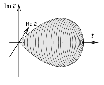
Figure 4: The surface of revolution over the nodal cubic

This construction admits the following generalization for some other values of the measure parameter. Namely, for $p=c/2$ where $c\in\{1,2,4,8\}$ (with $c=1$ corresponding to the considered model on ${\mathbb{S}}^{3}$). We shall use an interpretations similar to the one described in Section 4.6. Let us write a point in ${\mathbb{R}}^{3c+1}$ as $({\bf u},{\bf v},{\bf w})$, with ${\bf u},{\bf v}\in{\mathbb{R}}^{c}$ and ${\bf w}=(w_{0},w_{1},\dots,w_{c})\in{\mathbb{R}}^{c+1}$. Consider then $X=\|{\bf u}\|^{2}+\|{\bf v}\|^{2}$. For these values of $c$, as seen above, there exist $c$ orthogonal transformations $\ell_{k}$ in ${\mathbb{R}}^{c}$ such that $\{\ell_{1}({\bf v}),\ell_{2}({\bf v}),\dots,\ell_{c}({\bf v})\}$ is an orthonormal basis for any unit vector ${\bf v}\in{\mathbb{R}}^{c}$. Then, on ${\mathbb{R}}^{2c}$, one considers the bilinear functions $B_{k}({\bf u},{\bf v})=2{\bf u}\cdot\ell_{k}({\bf v})$, $k=1,\dots,c$, for which it is immediate that $\sum_{j=1}^{c}B_{j}^{2}=4\|{\bf u}\|^{2}\|{\bf v}\|^{2}$. Let also $B_{0}({\bf u},{\bf v})=\|{\bf u}\|^{2}-\|{\bf v}\|^{2}$. Then $\sum_{i=0}^{c}B_{i}^{2}=X^{2}$. For the Euclidean Laplacian on ${\mathbb{R}}^{2c}$, one has

$${\bf\Delta}_{\mathbb{E}}B_{i}=0,\qquad{\bf\Gamma}_{\mathbb{E}}(B_{i},B_{j})=4\delta_{ij}(\|{\bf u}\|^{2}+\|{\bf v}\|^{2}),\qquad i,j=0,\dots,c.$$

We then consider the function $Y=\sum_{i=0}^{c}w_{i}B_{i}$. For the Euclidean Laplace operator in ${\mathbb{R}}^{3c+1}$, one easily checks that ${\bf\Gamma}_{\mathbb{E}}(X,Y)=4Y$ and that

$${\bf\Gamma}_{\mathbb{E}}(Y,Y)=X^{2}+4X\|{\bf w}\|^{2}=X^{2}+4X(1-X).$$

The comparison (4.47) of spherical Laplace operator and the Euclidean one shows that the restrictions of $X$, $Y$, and the Laplace operator on the unit sphere in ${\mathbb{R}}^{3c+1}$ satisfy the required relations for ${\bf L}_{p}$ with $2p=c$.

It is perhaps worth to observe that in the above construction, the bilinear functions $B_{0},B_{1},\dots,B_{c}$, considered as functions on ${\mathbb{R}}^{2c}$ are harmonic and satisfy ${\bf\Gamma}_{\mathbb{E}}(B_{i},B_{i})=4\delta_{ij}(\|{\bf u}\|^{2}+\|{\bf v}\|^{2})$, and $\sum_{i}B_{i}^{2}=(\|{\bf u}\|^{2}+\|{\bf v}\|^{2})^{2}$ . Their restriction to ${\mathbb{S}}^{2c-1}$ satisfy then the same relations (up to some factor $4$) than the coordinates on a unit sphere ${\mathbb{S}}^{c}$. Any construction performed on those spheres may be then carried to ${\mathbb{S}}^{2c-1}$, just replacing $X_{i}$ by $B_{i}$.

4.9 The cuspidal cubic with one secant line

We may choose the boundary equation to be $(X^{3}-Y^{2})(X-1)=0$. Up to scaling, the associated metric is unique and we have

$$G=\begin{pmatrix}4X(1-X)&6Y(1-X)\\ 6Y(1-X)&9(X^{2}-Y^{2})\end{pmatrix}.$$

Since the boundary has degree 4, the Laplace operator associated with this metric belongs to the admissible solutions and we may check that the associated metric has constant scalar curvature $2$ and therefore may be realized from the unit sphere ${\mathbb{S}}^{2}$.

The general density measure is $\rho_{p,q}=(X^{3}-Y^{2})^{p-1}(1-X)^{q-1}$, $p>1/6$, for which we have for the associated operator ${\bf L}_{p,q}$

$${\bf L}_{p,q}(X)=-2(6p+2q-1)X+2(6p-1),\qquad{\bf L}_{p,q}(Y)=-3(6p+2q)Y.$$

For the Laplacian case, ${\bf L}_{1/2,\,1/2}$ is the image of ${\bf\Delta}_{{\mathbb{S}}^{2}}$ through

$$X=x_{1}^{2}+x_{2}^{2},\qquad Y=x_{1}\big{(}x_{1}^{2}-3x_{2}^{2}\big{)}.$$

The functions $F(X,Y)$ are the functions on the unit sphere which are invariant under $x_{3}\mapsto-x_{3}$ and such that the projection $z=x_{1}+ix_{2}=\rho e^{i\theta}$ on the hyperplane $\{x_{3}=0\}$ depend only on $\rho$ and $\cos(3\theta)$. These are the functions which are invariant under symmetries through the hyperplanes $H=\{x_{2}=0\}$ and the two hyperplanes having an angle $\pm\pi/3$ with $H$. The fundamental domain for these symmetries on the sphere is a triangle with angles $(\pi/3,\pi/2,\pi/2)$, which correspond to one cusp and two double points.

For the other density measures, we may consider the unit sphere in ${\mathbb{R}}^{3c+2}\times{\mathbb{R}}^{2q}$ where $2p=c+1$. For a point $({\bf u},{\bf v})\in{\mathbb{R}}^{3c+2}\times{\mathbb{R}}^{2q}$, we set $X=\|{\bf u}\|^{2}$ and we chose for $Y$ some homogeneous degree 3 harmonic polynomial $P({\bf u})$. Then, the required formulae for ${\bf L}_{p,q}(X)$, ${\bf L}_{p,q}(Y)$, ${\bf\Gamma}(X,X)$, ${\bf\Gamma}(X,Y)$ and ${\bf\Gamma}(Y,Y)$ are satisfied as soon as ${\bf\Gamma}_{\mathbb{E}}(Y,Y)=9\|{\bf u}\|^{4}$, where ${\bf\Gamma}_{\mathbb{E}}$ denotes the Euclidean operator ${\bf\Gamma}$.

This problem has been studied by Cartan [15] where he proved that such polynomials exist only for $c=0,1,2,4,8$. Beyond the case $c=0$ (the above example), this corresponds respectively to real, complex, quaternionic and octonionic structures. Such a function (for $c=1,2,4,8$ ) may be for example represented as follows: consider a Hermitian $3\times 3$ matrix with trace $0$ and respectively real, complex, quaternionic, or octonionic entries. On this space of matrices, one may consider the Euclidean structure given by $X=\|M\|^{2}=\textmd{trace}\,(M^{*}M)$, and, for this structure, the function $Y:M\mapsto 3\sqrt{6}\det(M)$, satisfies $\|M\|^{2}=\textmd{trace}\,(M^{2})$, as one may check by direct computation. The case $p=0$ corresponds to diagonal matrices.

Remark 4.5.

The determinant of a $3\times 3$ Hermitian matrix over ${\mathbb{H}}$ or ${\mathbb{O}}$, in fact, does not make much troubles. Indeed, only two terms of its expansion depend on the order of multiplication: $M_{12}M_{23}M_{31}$ and $M_{13}M_{32}M_{21}$. So, we can choose any order for one of them and take the conjugate value for the other one.

4.10 The cuspidal cubic with one tangent

We may choose the boundary equation to be

$$(X^{3}-Y^{2})(2Y-3X+1))=0$$

(one can write the second factor in the form $2(Y-1)-3(X-1)\,$). Then, up to scaling, there is a unique solution

$$G=2\begin{pmatrix}4(X+Y-2X^{2})&6(Y-2XY+X^{2})\\ 6(Y-2XY+X^{2})&9(X-Y)(X+2Y)\end{pmatrix}.$$

The boundary having degree $4$, the density measure $\det(G)^{-1/2}$ belongs to the admissible solutions. Therefore, the Laplace operator associated with this (co)-metric is an admissible solution. The scalar curvature is $2$, and therefore we may realize this Laplace operator as an image of the spherical Laplacian ${\bf\Delta}_{{\mathbb{S}}^{2}}$.

The general density measure is $\rho=(X^{3}-Y^{2})^{p-1}(2Y-3X+1)^{q-1}$, $p>1/6$, $q>0$, $p+q>1/2$. For this measure we have

$${\bf L}_{p,q}(X)=\;-8(6p+3q-2)X+4(6p-1),$$

$${\bf L}_{p,q}(Y)=-12(6p+3q-1)Y+6(6p+1)X.$$

In the case $p=q=1/2$, which corresponds to the Laplace operator, one may see that the operator is the image of a two-dimensional sphere, where $X$ is a degree $4$ polynomial and $Y$ has degree $6$. Indeed, it is worth to represent $X$ and $Y$ as

$$X=-\tfrac{1}{3}(t_{1}t_{2}+t_{2}t_{3}+t_{3}t_{1})\qquad\text{and}\qquad Y=\tfrac{1}{2}t_{1}t_{2}t_{3}$$ (4.55)

with $t_{1}+t_{2}+t_{3}=0$, which reflects the fact that $X^{3}-Y^{2}$ (up to scaling) is the discriminant of the polynomial $T^{3}-3XT+2Y$.

A solution is given by $t_{i}=3x_{i}^{2}-1$, and one may check that all the relations concerning ${\bf L}_{1/2,\,1/2}(X)$, ${\bf L}_{1/2,\,1/2}(Y)$, ${\bf\Gamma}(X,X)$, ${\bf\Gamma}(X,Y)$ and ${\bf\Gamma}(Y,Y)$ are satisfied for this choice (on the $2$-sphere $x_{1}^{2}+x_{2}^{2}+x_{3}^{2}=1$).

From this representation, it is clear that $X$ and $Y$ are invariant under the symmetries through the hyperplanes $\{x_{i}=0\}$ and $\{x_{i}=x_{j}\}$. The fundamental domain for those reflexions is a triangle on the sphere, defined by the hyperplane coordinates, cut along its three medians, with angles $\pi/2,\pi/3,\pi/4$. This corresponds to one double point, one cusp and one tangency point.

In the case when $p=1/2$ and $q$ is a positive half-integer, we may take a unit sphere in ${\mathbb{R}}^{n}$, $n=6q$, whose elements we represent by triples $({\bf x}_{1},{\bf x}_{2},{\bf x}_{3})$ with ${\bf x}_{j}\in{\mathbb{R}}^{2q}$. and consider $X$ and $Y$ given by (4.55) but with $t_{j}=3\|{\bf x}_{j}\|^{2}-1$, $j=1,2,3$. Then, for the spherical Laplace operator on ${\mathbb{S}}^{n-1}$ one can check that ${\bf\Gamma}(X,X)$, ${\bf\Gamma}(X,Y)$ and ${\bf\Gamma}(Y,Y)$, ${\bf L}_{p,q}(X)$ and ${\bf L}_{p,q}(Y)$ satisfy the required equations. It is certainly worth to mention that this model may also be seen as the image of the triangle model (Section 4.4) on the triangle $\{(s_{1},s_{2},s_{3})\in{\mathbb{R}}^{3}\mid s_{1}+s_{2}+s_{3}=1,~{}s_{i}\geq 0\}$ through the transformation $X=s_{1}s_{2}+s_{2}s_{3}+s_{3}s_{1},~{}Y=s_{1}s_{2}s_{3}$.

For $p=1$ and a positive half-integer $q$, one may consider the following model. For $({\bf x}_{1},{\bf x}_{2},{\bf x}_{3})\in{\mathbb{R}}^{n}$, $n=6+6q$, ${\bf x}_{j}\in{\mathbb{R}}^{2+2q}$, we consider the $3\times 3$ symmetric matrix $M_{ij}=({\bf x}_{i}\cdot{\bf x}_{j})-\frac{1}{3}\delta_{ij}$. Then the restriction of this matrix to the unit sphere in ${\mathbb{R}}^{n}$ has trace $0$, and one considers its characteristic polynomial $P(\lambda)=\det(\lambda\,\textmd{Id}\,-M)$. Write $P(\lambda)=\lambda^{3}-\frac{1}{3}\lambda X-\frac{2}{27}Y$. Then the image of the operator ${\bf\Delta}_{{\mathbb{S}}^{n-1}}$ is ${\bf L}_{p,q}$.

This is case $c=1$ of a construction which works for $c=\dim_{{\mathbb{R}}}{\mathbb{K}}$ where ${\mathbb{K}}$ is ${\mathbb{R}}$, ${\mathbb{C}}$, or ${\mathbb{H}}$. In each of these three cases we consider $({\bf x}_{1},{\bf x}_{2},{\bf x}_{3})$ with ${\bf x}_{j}\in{\mathbb{K}}^{m}$, $m\geq 3$, and define $M$, $X$, and $Y$ as above but with ${\bf x}\cdot{\bf y}$ understood as the Hermitiant product $\sum_{j=1}^{m}x_{i}\bar{y}_{i}$ (see also Remark 4.5). Then the projection of ${\bf\Delta}_{{\mathbb{S}}^{n-1}}$, $n=3cm$, yields ${\bf L}_{p,q}$ with $2p=c+1$ and $2q=c(m-2)$ (recall that $c\in\{1,2,4\}$ and $m\geq 3$). It could be interesting to generalize this construction for the octonions. A computation shows that literally the same formulas do not lead to the desired result.

4.11 The swallow tail

This is a degree $4$ algebraic curve, whose, up to affine transformations, we may chose the equation to be

$$4\,X^{2}-27\,X^{4}+16\,Y-128\,Y^{2}-144\,X^{2}Y+256\,Y^{3}=0.$$

This is the discriminant in $T$ of the polynomial $T^{4}-T^{2}+XT+Y$. Once again, the metric is unique up to scaling, and we have

$$G=\begin{pmatrix}2-8Y-9X^{2}&-X(12Y+1)\\ -X(12Y+1)&\frac{3}{2}X^{2}-16Y^{2}+4Y\end{pmatrix}.$$

The boundary having degree $4$, the measure density $\det(G)^{-1/2}$ is an admissible solution, and for this measure, the corresponding Laplace operator has constant scalar curvature $2$, and therefore the operator may be represented on the unit sphere ${\mathbb{S}}^{2}$.

The general measure density is $\rho=\det(G)^{p-1}$, $p>1/6$. For it we have

$${\bf L}_{p}(X)=-6(6p-1)X,\qquad{\bf L}_{p}(Y)=-4(12p-1)Y+4p-1.$$

In the Laplace-Beltrami case

$${\bf L}_{1/2}(X)=-12X,\qquad{\bf L}_{1/2}Y=1-20Y,$$

which corresponds for $X$ to be an eigenvector of degree $3$ and $Y-1$ to be an eigenvector of degree $4$.

Taking in account that the boundary is a discriminant, we should look for

$$-X=t_{1}t_{2}t_{3}+t_{2}t_{3}t_{4}+t_{3}t_{4}t_{1}+t_{4}t_{1}t_{2},\qquad Y=t_{1}t_{2}t_{3}t_{4},$$

on the variety given by

$$t_{1}+t_{2}+t_{3}+t_{4}=0,\qquad\sum_{i<j}t_{i}t_{j}=-1.$$

Since $\sum t_{i}^{2}=\big{(}\sum t_{i}\big{)}^{2}-2\sum t_{i}t_{j}$, this variety is the intersection of a sphere ${\mathbb{S}}^{3}$ of radius $\sqrt{2}$ with the hyperplane $\{\sum t_{i}=0\}$, which is again a sphere with radius $\sqrt{2}$.

To compute the image of ${\bf\Delta}_{\Sigma}$ through $(X,Y)$, we introduce the following orthogonal coordinates on the plane $\sum t_{i}=0$:

$$\begin{matrix}t_{1}=(x_{1}+x_{2}+x_{3})/\sqrt{2}\,,\quad&t_{3}=(-x_{1}+x_{2}-x_{3})/\sqrt{2}\,,\\ t_{2}=(x_{1}-x_{2}-x_{3})/\sqrt{2}\,,\quad&t_{4}=(-x_{1}-x_{2}+x_{3})/\sqrt{2}\,\end{matrix}$$

where the scaling factor $\sqrt{2}$ is chosen so that the unit 2-sphere ${\mathbb{S}}^{2}$ in ${\mathbb{R}}^{3}$ with coordinates ${\bf x}=(x_{1},x_{2},x_{3})$ is mapped onto $\Sigma$. In these coordinates we have $X=2\sqrt{2}\,x_{1}x_{2}x_{3}$ and $Y=\frac{1}{2}(x_{1}^{4}+x_{2}^{4}+x_{3}^{4})-\frac{1}{4}\|{\bf x}\|^{4}$, thus the restriction of $Y$ to ${\mathbb{S}}^{2}$ is $\frac{1}{2}(x_{1}^{4}+x_{2}^{4}+x_{3}^{4})-\frac{1}{4}$. Then the image of ${\bf\Delta}_{{\mathbb{S}}^{2}}$ through $(X,Y)$ can be easily computed using (4.47) and the result will be ${\bf L}_{1/2}$.

For other values of $p$, the discriminant form of the boundary suggests that one looks at Hermitian $4\times 4$ matrices $M$ with vanishing trace, restricted on the sphere $\textmd{trace}\,(M^{*}M)=2$, embedded with the induced spherical structure, in the real and complex cases, and look at the induced operator on the characteristic polynomial $P(\lambda)=\lambda^{4}-\lambda^{2}+\lambda X+Y$. Then the image of $\Delta_{S^{2+6c}}$ ($c=1$ for ${\mathbb{R}}$ and $c=2$ for ${\mathbb{C}}$) through $(X,Y)$ is ${\bf L}_{p}$ with $2p=c+1$. The quaternionic case is left to the reader as an exercise ([8] can be used as a hint).

Observe also that the mapping $(X,Y)\mapsto(X^{2},Y)$ transforms all these models into some models for the cuspidal cubic with tangent (indeed, the spherical triangle with angles $(\frac{\pi}{2},\frac{\pi}{3},\frac{\pi}{3})$ folded along its axis of symmetry yields a triangle with the angles $(\frac{\pi}{2},\frac{\pi}{3},\frac{\pi}{4})$).

4.12 The deltoid

In this case, up to affine transformation, we may choose the boundary equation to be

$$(X^{2}+Y^{2})^{2}+18(X^{2}+Y^{2})-8X^{3}+24XY^{2}-27=0.$$

There is a unique metric $g$ up to scaling, which is

$$G=\begin{pmatrix}9+6X+Y^{2}-3X^{2}&-2Y(2X+3)\\ -2Y(2X+3)&9-6X+X^{2}-3Y^{2}\end{pmatrix}.$$

For the density measure $\rho=\det(G)^{p-1}$, $p>1/6$, we have

$${\bf L}_{p}(X)=-2(6p-1)X,\qquad{\bf L}_{p}(Y)=-2(6p-1)Y.$$

The operator looks simpler in complex variables: setting $Z=X+iY$, one gets

$${\bf\Gamma}(Z,Z)=12\bar{Z}-4Z^{2},\qquad{\bf\Gamma}(Z,\bar{Z})=18-2Z\bar{Z},\qquad{\bf\Gamma}(\bar{Z},\bar{Z})=12Z-4\bar{Z}^{2},$$

and

$${\bf L}_{p}(Z)=-2(6p-1)Z,\qquad{\bf L}_{p}(\bar{Z})=-2(6p-1)\bar{Z}.$$

Under this form, it is easier to check the eigenvalues for ${\bf L}_{p}$, since the action of the operator on the highest degree term of a polynomial is diagonal, and we see that, for any degree $p$, the highest degree part of any eigenvector is a monomial, say $Z^{q}\bar{Z}^{r}$, and the same use of complex variables gives that the eigenvalue corresponding to a polynomial whose highest degree term is $Z^{p}\bar{Z}^{q}$ is $-3(q+r)(q+r+4p+2)-(q-r)^{2}$.

Once again, as it is the case whenever the boundary is degree $4$, the density measure $\det(G)^{-1/2}$ is an admissible solution, and this corresponds to a Laplace operator for a metric which has zero scalar curvature. We may represent this operator from a Euclidean Laplacian in dimension 2. For this choice of the measure, one has ${\bf L}_{1/2}(Z)=-4Z$, and if we identify ${\mathbb{R}}^{2}$ with the complex plane ${\mathbb{C}}$, one may represent this using

$$Z=e^{2i(1\cdot z)}+e^{2i(\omega\cdot z)}+e^{2i(\bar{\omega}\cdot z)},$$

where $z=x+iy\in{\mathbb{C}}$, $1$, $\omega$, $\bar{\omega}$ are the three third roots of unity (solution of $z^{3}=1$) and $z_{1}\cdot z_{2}$ is the Euclidean scalar product $\textmd{Re}\,(z_{1}\bar{z}_{2})$. One may directly check the ${\bf L}_{1/2}$ is the image of ${\bf\Delta}_{{\mathbb{R}}^{2}}$ through $Z$. (The interior of the deltoid is indeed the image of ${\mathbb{R}}^{2}$ through $Z$.) Moreover, the function $Z$ is invariant under the symmetries with respect to the lines

$$D_{1}=\{\textmd{Im}\,(z)=0\},\qquad D_{2}=\{te^{i\pi/3},t\in{\mathbb{R}}\},\qquad D_{3}=\{ae^{i\pi/6}+te^{2i\pi/3}\},$$

with $a=\pi/\sqrt{3}$. Those three lines determine a equilateral triangle $(ABC)$ in the plane, and any function which has those symmetries is also invariant under all the symmetries with respect to the lines of the triangular lattice generated by $A,B,C$ (that is all the lines parallel to $D_{1}$, $D_{2}$, $D_{3}$ which are distant from $ka$, $k\in{\mathbb{N}}$). (This group of symmetries is the affine Weyl group associated with the root system $A_{2}$.

The deltoid is then the image of the boundary of the triangle $(ABC)$ through $Z$, and it is not hard to see that the restriction of $Z$ to $(ABC)$ is injective. Then, the functions of the form $F(Z)$ are nothing else than the functions which are invariant under the symmetries of the triangular lattice, and ${\bf L}_{1/2}$ is just ${\bf\Delta}$ acting on functions invariant under the affine Weyl group associated with $A_{2}$.

As usual, this model extends to rank 2 symmetric spaces with restricted root system $A_{2}$. For a study of this case, see also Koornwinder [47, 48]. Indeed, it is perhaps worth to notice that the boundary equation is the discriminant of the polynomial $T^{3}-ZT^{2}+\bar{Z}T+1$, putting forward the interest of representing $Z$ as $\lambda_{1}+\lambda_{2}+\lambda_{3}$ where $|\lambda_{i}|=1$ and $\lambda_{1}\lambda_{2}\lambda_{3}=1$. In particular, one may consider the Casimir operator on $SU(3)$. Indeed, if $Z$ denotes the trace of a $SU(3)$ matrix, due to the fact that eigenvalues $(\lambda_{1},\lambda_{2},\lambda_{3})$ satisfy $|\lambda_{i}|=1$, $\lambda_{1}\lambda_{2}\lambda_{3}=1$, one sees that the characteristic polynomial $P(\lambda)$ writes $P(\lambda)=-\lambda^{3}+Z\lambda^{2}-\lambda\bar{Z}+1$. Then, using formulae (4.49) and (4.50), one sees that

$${\bf\Delta}_{SU(3)}Z=-\tfrac{16}{3}Z,\qquad{\bf\Delta}_{SU(3)}\bar{Z}=-\tfrac{16}{3}\bar{Z},$$

and

$${\bf\Gamma}_{SU(3)}(Z,Z)=\tfrac{4}{3}(3\bar{Z}-Z^{2}), ~{}{\bf\Gamma}_{SU(3)}(Z,Z)=\tfrac{4}{3}(3Z-\bar{Z}^{2}),$$

$${\bf\Gamma}_{SU(3)}(Z,\bar{Z}))=\tfrac{2}{3}({Z\bar{Z}}-9),$$

which shows that ${\bf L}_{3/2}$ is the image of $3{\bf\Delta}_{SU(3)}$ through $Z$.

It is worth to observe that this operator preserves the functions which are symmetric under the conjugacy $Z\mapsto\bar{Z}$. Indeed, choosing as new variables $X=Z+\bar{Z}$ and $Y=Z\bar{Z}$, one gets for the cometric ${\bf\Gamma}$ in those variables

$$\begin{pmatrix}1+X-X^{2}+Y&\frac{1}{2}X+X^{2}-2Y-\frac{3}{2}XY\\ \frac{1}{2}X+X^{2}-2Y-\frac{3}{2}XY&Y-3XY-3Y^{2}+X^{3}\end{pmatrix}$$

with

$${\bf L}X=-\lambda X,\qquad{\bf L}(Y)=1-(2\lambda+1)Y.$$

The determinant of this matrix is, up to some constant, $(4X-Y^{2})(4X^{3}-3Y^{2}-12XY-6Y+1)$, which corresponds to a domain delimited by a parabola and a cuspidal cubic which have a double tangent at their intersection points (and is a degree 5 curve). This domain is the image of the deltoid domain through the map $(X,Y)$. We may now describe a two parameters family of orthogonal polynomials associated with this domain, but with a weighted degree $\deg(X^{p}Y^{q})=2p+q$. For the associated Laplace operator, this corresponds to the 2 dimensional Euclidean Laplacian associated with the symmetries of the root system $G_{2}$.

5 The full ${\mathbb{R}}^{2}$ case

In this Section, we consider the case where $\Omega={\mathbb{R}}^{2}$, and concentrate on the SDOP problem. From the one dimensional models and the tensorization procedure, we already know that Gaussian measures provide such orthogonal polynomials, with the two-dimensional Ornstein-Uhlenbeck operator as associated diffusion operator. We shall prove in this section the following

Theorem 5.1.

If $({\mathbb{R}}^{2},G,\rho dx)$ is a solution of the SDOP problem, then, up to an affine change of coordinates, one has $\rho=\frac{1}{2\pi}\exp(-\frac{1}{2}(X^{2}+Y^{2}))$, and

$$G=\begin{pmatrix}a+\mu X^{2}&-\mu XY\\ -\mu XY&c+\mu Y^{2}\end{pmatrix},$$

where $a$ and $c$ are positive real numbers. The corresponding operator ${\bf L}$ is a sum of the general Ornstein-Uhlenbeck operator

$$L_{a,c}=a(\partial^{2}_{X}-X\partial_{X})+c(\partial^{2}_{Y}-Y\partial_{Y})$$

and a squared rotation $\mu(Y\partial_{X}-X\partial_{Y})^{2}$.

In this situation, we do not have boundary equation to restrict the analysis of the (co-)metric $(G^{ij})$. We therefore look for $3$ polynomials $G^{11},G^{12},G^{22}$ of degree at most $2$ in the variables $(X,Y)$ with $\Delta=G^{11}G^{22}-(G^{12})^{2}>0$ on $\mathbb{R}^{2}$ and for a function $h$ such that for the measure $d\rho=e^{h}dXdY$, the polynomials of $(X,Y)$ are dense in ${\cal L}^{2}(\rho,\mathbb{R}^{2})$. From (2.18), there exists $L_{X}$ and $L_{Y}$ affine forms in $\mathbb{R}^{2}$ such that

$$\partial_{X}h=\frac{G^{22}L_{X}-G^{12}L_{Y}}{\Delta},~{}\partial_{Y}h=\frac{-G^{12}L_{X}+G^{11}L_{Y}}{\Delta}$$ (5.56)

Let us first show that $\Delta$ has degree at most $2$. If $\Delta$ is of degree $4$, and since $\Delta>0$ on $\mathbb{R}^{2}$, there is at least a cone in which, for some constant $c$, $\Delta\geq c(X^{2}+Y^{2})^{2}$ at infinity and $d\rho$ cannot integrate any polynomial. Hence $\Delta$ is of degree at most $3$ and since it is positive on $\mathbb{R}^{2}$, $\Delta$ is of an even degree, thus of degree $2$ or zero.

5.1 Case where $\Delta$ is degree 2

Let us first consider the case where $\Delta$ is complex irreducible. From the form of the measure (Proposition 2.15), we know that

$$h=\log\rho=-P-\alpha\log\Delta,$$ (5.57)

where $P$ is a polynomial with degree at most $2$. The terms of highest degrees in $P$ is a positive definite quadratic form. Indeed, otherwise the measure $\rho\,dx$ would not integrate the polynomials. Thus $\deg P=2$.

Let us show that $\alpha=0$. Indeed, suppose that $\alpha\neq 0$. Then by Proposition 2.17 $(G^{11},G^{12},G^{22},\Delta)$ is a solution of the ${\mathbb{R}}$-AlgDOP problem (see Definition 3.2). Since $\deg\Delta=2$ and $\Delta\neq 0$ on ${\mathbb{R}}^{2}$, up to affine linear transformation, we have either $\Delta=X^{2}+Y^{2}+1$ or $\Delta=X^{2}+1$. Then Proposition 3.19 and Lemma 3.22 imply that

$$G=\begin{pmatrix}1+X^{2}&XY\\ XY&1+Y^{2}\end{pmatrix}\qquad\text{or}\qquad G=\begin{pmatrix}1+X^{2}&0\\ 0&1\end{pmatrix}$$

(we do the change of coordinates $X=ix$, $Y=iy$ in the corresponding solution in Proposition 3.19 and Lemma 3.22). Thus condition (2.15) takes the form

$$(1+X^{2})\,\partial_{X}P+XY\,\partial_{Y}P=L_{X},\qquad XY\,\partial_{X}P+(1+Y^{2})\,\partial_{Y}P=L_{Y},$$

or, respectively,

$$(1+X^{2})\,\partial_{X}P=L_{X},\qquad\,\partial_{Y}P=L_{Y},$$

with $\deg L_{X}\leq 1$ and $\deg L_{Y}\leq 1$. One easily checks that in both cases this is possible only when $P$ is a constant which contradicts the condition $\deg P=2$. Thus $\alpha=0$.

Recall that the highest order homogeneous component of $P$ is a positive definite quadratic form. Hence by an affine change of coordinates we may reduce to the case $P=(X^{2}+Y^{2})/2$. Then condition (2.15) reads

$$G^{11}X+G^{12}Y=L_{X},\qquad G^{21}X+G^{22}Y=L_{Y},\qquad$$

with $\deg L_{X}\leq 1$ and $\deg L_{Y}\leq 1$. This is a linear system on the coefficients of $G^{ij}$. By solving it, we obtain, up to a scalar factor,

$$G=\begin{pmatrix}a+Y^{2}&b-XY\\ b-XY&c+X^{2}\end{pmatrix},$$

with some constant positive definite matrix $\begin{pmatrix}a&b\\ b&c\end{pmatrix}$ and the associated operator is the sum of the general Ornstein-Uhlenbeck operator

$$L_{a,b,c}=a\partial^{2}_{X}+2b\,\partial_{X}\partial_{Y}+c\partial^{2}_{Y}-(aX+bY)\partial_{X}-(bX+cY)\partial_{Y}$$

and a plane squared rotation $(Y\partial_{X}-X\partial_{Y})^{2}$.

With a further rotation, one may reduce to the case where $b=0$.

5.2 $\Delta$ is constant

We can boil down to $\Delta=1$. Our aim is to prove in this section that $G^{ij}$ are constant – in this case (5.56) implies that $P$ is of degree 2 which corresponds to Ornstein-Uhlenbeck operators. Suppose that $G$ is non-constant. Then one of $G^{11}$, $G^{22}$ is non-constant. Let it be $G^{11}$.

Since $\Delta=1$, we have $G^{11}G^{22}=(G^{12}-i)(G^{12}+i)$. If $G^{11}$ is irreducible, then $G^{11}=\lambda(G^{12}\pm i)$, which is impossible since $G^{11}$ is real. Therefore, $G^{11}=l_{1}l_{2}$ with $\deg l_{1}=\deg l_{2}=1$. Since $G^{11}>0$ on ${\mathbb{R}}^{2}$, the only solution is $G^{11}=(l_{a}+\alpha)(l_{a}+\bar{\alpha})$ where $l_{a}$ is a nonzero real linear form and $\alpha$ is a non-real complex number. Similarly, $G^{22}=(l_{c}+\gamma)(l_{c}+\bar{\gamma})$, where $l_{c}$ is a real linear form, and if $l_{c}$ is nonzero, then $\gamma$ is a non-real complex number. Hence, changing if necessary the sign of $l_{c}+\gamma$, we have

$$G^{12}+i=(l_{a}+\alpha)(l_{c}+\gamma),\qquad G^{12}-i=(l_{a}+\bar{\alpha})(l_{c}+\bar{\gamma}).$$

We know that $(l_{a}+\alpha)(l_{c}+\gamma)\pm i$ is a real polynomial. Hence all its homogeneous forms are real, in particular, its linear form is real, i.e., $\alpha l_{c}+\gamma l_{a}=\bar{\alpha}l_{c}+\bar{\gamma}l_{a}$ whence

$$(\alpha-\bar{\alpha})l_{c}=(\bar{\gamma}-\gamma)l_{a}.$$

Since $\alpha$ is non-real, we obtain $l_{c}=\nu l_{a}$ for some real number $\nu$. From now on we denote $l_{a}$ just by $l$. So, we have

$$\begin{pmatrix}G^{11}&G^{12}\\ G^{12}&G^{22}\end{pmatrix}=\begin{pmatrix}l^{2}+(\alpha+\bar{\alpha})l+\alpha\bar{\alpha}&\nu l^{2}+c\,l+b\\ \nu l^{2}+c\,l+b&\nu^{2}l^{2}+\nu(\gamma+\bar{\gamma})l+\gamma\bar{\gamma}\end{pmatrix},$$

where $l$ is some real non zero linear form, $\nu$, $c=(\alpha\nu+\gamma)$, $b=\alpha\gamma-i$ are real numbers whereas $\alpha$ and $\gamma$ some non-real complex numbers.

Assume first that $\nu\neq 0$. Then one may reduce to the case $c=0$ through a translation, and eventually to the case that $\nu=\alpha\bar{\alpha}=\gamma\bar{\gamma}=1$, $b=0$, through a linear change of coordinates. In this case, the determinant is easy to compute and the only solution, up to a change of $Y$ into $-Y$ and an exchange of $X$ and $Y$, is

$$\begin{pmatrix}G^{11}&G^{12}\\ G^{12}&G^{22}\end{pmatrix}=\begin{pmatrix}l^{2}+\sqrt{2}\,l+1&l^{2}\\ l^{2}&l^{2}-\sqrt{2}\,l+1\end{pmatrix}.$$

Let us show that then the measure $\rho\,dx$ cannot be integrable.

We know from Proposition 2.15 that $\rho=\exp(P)dx$, where $P$ is some polynomial of degree at most $4$. By (2.18) we have

$$\begin{pmatrix}G^{11}&G^{12}\\ G^{12}&G^{22}\end{pmatrix}\begin{pmatrix}\partial_{X}P\\ \partial_{Y}P\end{pmatrix}=\begin{pmatrix}l_{X}+c_{X}\\ l_{Y}+c_{Y}\end{pmatrix},$$

where $l_{X}$ and $l_{Y}$ are linear forms, and $c_{X}$ and $c_{Y}$ are constants.

From this, we get

$$\begin{pmatrix}\partial_{X}P\\ \partial_{Y}P\end{pmatrix}=\begin{pmatrix}G^{22}&-G^{12}\\ -G^{12}&G^{11}\end{pmatrix}\begin{pmatrix}l_{X}+c_{X}\\ l_{Y}+c_{Y}\end{pmatrix}.$$

Writing $P=P_{4}+P_{3}+P_{2}+P_{1}+P_{0}$ where $P_{k}$ is homogeneous of degree $k$, one sees from this equation that $(\partial_{X}+\partial_{Y})P_{4}=0$. Since the measure has to be integrable, this also requires that $(\partial_{X}+\partial_{Y})P_{3}=0$. But, looking precisely at $(\partial_{X}+\partial_{Y})P_{3}$, we see that it is equal to $-\sqrt{2}\,l(l_{X}-l_{Y})$, thus $l_{X}-l_{Y}=0$. From this, one sees that $\partial_{X}P_{4}=\partial_{Y}P_{4}=0$, and hence $P_{4}=0$. This implies that $P_{3}=0$ too (since once again the measure has to be finite). We have

$$\partial_{X}P_{3}=(c_{X}-c_{Y})l^{2}-\sqrt{2}\,l\,l_{X},\qquad-\partial_{Y}P_{3}=(c_{X}-c_{Y})l^{2}-\sqrt{2}\,l\,l_{Y},$$

thus $P_{3}=0$ implies $l_{X}=l_{Y}=\frac{\sqrt{2}}{2}(c_{X}-c_{Y})l$. Since $\partial_{X}P_{2}=l_{X}-\sqrt{2}\,c_{X}l$ and $\partial_{Y}P_{2}=l_{Y}+\sqrt{2}\,c_{Y}l$, we obtain $\partial_{X}P_{2}=-\partial_{Y}P=-\frac{\sqrt{2}}{2}(c_{X}+C_{Y})l$ whence $(\partial_{X}+\partial_{Y})P_{2}=0$. Therefore $P_{2}$ is a degenerate quadratic form, and $\exp(P)$ is non integrable on ${\mathbb{R}}^{2}$.

In the case where $\nu=0$ with the same argument, we boil down to

$$\begin{pmatrix}G^{11}&G^{12}\\ G^{12}&G^{22}\end{pmatrix}=\begin{pmatrix}l^{2}+1&l\;\\ l&1\;\end{pmatrix}.$$

The same reasoning shows that the measure may not be integrable on ${\mathbb{R}}^{2}$.

6 Non compact cases with boundaries.

(1)                (2)            (3)         (4)          (5)        (6)      (7)

In this section, we again consider the SDOP problem, which is perhaps not enough to describe all the possible solutions of the general DOP problem (although we have no example of solution of the latter beyond the cases described here).

We describe all the possible models, but we do not give any geometric interpretation, and do not detail for which values of the parameters appearing in the measure the polynomials are dense in ${\cal L}^{2}(\mu)$. However, in all the cases described below, it is indeed the case for at least some values of these parameters. Moreover, one could give a geometric construction for many models as images of Ornstein-Uhlenbeck operators in some Euclidean space, associated with Gaussian measures.

Following the results of Section 2, we reduce to the cases where every factor $\Delta_{p}$ appearing in the boundary satisfies the fundamental equations (2.22). We also need, for the measure $d\mu=e^{h}dx$, that ${\cal L}^{2}(\mu)$ contains every polynomial. Hence in any case, we have to look for the existence of such a measure, which will turn out to be the main restriction. We indeed require more, namely that polynomials are dense in ${\cal L}^{2}(\mu)$. We know from Proposition 2.15 the general form of the measure. In addition to the boundary terms, there appear in $h$ a polynomial term $P$ which will be crucial when integrating the polynomials on the domain (see previous section) . This constraint will help us to restrict the number of cases for the metric $(G)$. Moreover, if the determinant $\Delta$ of $(G)$ has no multiple factors and the domain contains an open cone, the degree of $\Delta$ is at most $3$. When there are multiple factors, the same kind of analysis can be undergone.

The algebraic analysis undergone in Section 3 still holds, and produces the following list of possible boundaries.

1. $\partial\Omega=\{Y^{2}-X^{3}=0\}$. In this case, the general metric is given by

   $$G=\alpha\begin{pmatrix}4X^{2}&6XY\\ 6XY&9Y^{2}\end{pmatrix}+\beta\begin{pmatrix}4X&6Y\\ 6Y&9X^{2}\end{pmatrix}+\gamma\begin{pmatrix}4Y&6X^{2}\\ 6X^{2}&9XY\end{pmatrix}$$

   Here, the determinant $\Delta$ is $36(X^{3}-Y^{2})\big{(}(\alpha\beta-\gamma^{2})X-\alpha\gamma Y+\beta^{2}\big{)}$. By Corollary 2.25 we have $\deg\Delta\leq 3$, hence $\alpha=\gamma=0$, and by homogeneity we may restrict to $\beta=1$. Since $\Delta>0$ in the interior of the domain $\Omega$, one sees that the domain must be $X^{3}>Y^{2}$. This leads to measures on the domain $X^{3}>Y^{2}$ of the form

   $$d\mu_{a,b}=C_{a,b}(X^{3}-Y^{2})^{a-1}\exp(-bX)\,dXdY,\quad a>1/6,\;\;b>0..$$

2. $\partial\Omega=\{Y-X^{2}=0\}$. Then $\Delta=(Y-X^{2})\Delta_{1}$ where, by Corollary 2.25, either $\Delta_{1}$ is proportional to $(Y-X^{2})$, or $\deg\Delta_{1}\leq 1$.

   1. $\Delta=c(Y-X^{2})^{2}$. In this case, the general metric is given in Proposition 3.21(1). We may show that there is no finite measure solution for the problem.

   2. $\deg\Delta=3$ (cf. Proposition 3.21(2)). The metric for which there exist a measure solution for the problem may be written as

      $$G=\begin{pmatrix}1+\alpha(Y-X^{2})&2X\\ 2X&4Y\end{pmatrix},\qquad\alpha>0.$$ (6.58)

      We have $\det G=4(Y-X^{2})(1+\alpha Y)$, this is why we impose the condition $\alpha>0$. By a change of coordinates $X\mapsto cX,Y\mapsto c^{2}Y$, we may reduce to $\alpha=1$. The existence of a finite measure solution imposes $\Omega=\{Y>X^{2}\}$ and measures to be

      $$(Y-X^{2})^{a-1}\exp\big{(}-bY\big{)}dXdY,\quad a,b>0.$$

   3. $\Delta$ has degree $2$. The only metric for which there exists a measure solution is (6.58) with $\alpha=0$. This is a limit case of the previous one. Notice that any measure of the form $(Y-X^{2})^{a-1}\exp\big{(}-bY+cY\big{)}dXdY$ with $a,b>0$ is admissible in this case. However we may reduce to $c=0$ by $(X,Y)\mapsto(X+q,Y+2qX+q^{2})$ which is an isometry of $(\Omega,g)$.

3. $\Omega$ is bounded by $\{Y-X^{2}=0\}$ and a line. Up to an affine linear transformation, it is enough to consider the following three cases for the line.

   1. $\partial\Omega\subset\{Y(Y-X^{2})=0\}$. Then the metric is (3.41) with $\beta=\gamma=\lambda=0$. If $\Delta$ has a multiple factor, then $r=0$. One can check that a finite admissible measure does not exist.

      If there are no multiple factors of $\Delta$, then the integrability condition implies $\deg\Delta=3$ (see Corollary 2.25). This occurs only for $\alpha=\mu=0$, hence

      $$G=r\begin{pmatrix}X&2Y\\ 2Y&4XY\end{pmatrix}.$$

      This matrix is positive definite in $\Omega=\{rX>0$ and $0<Y<X^{2}\}$. The admissible measures for $r>0$ are

      $$C\,Y^{a-1}(X^{2}-Y)^{b-1}\,\exp(-cX),\quad a,b,c>0,\quad a+b>1/2.$$

   2. $\partial\Omega\subset\{X(Y-X^{2})=0\}$. The metric is (3.41) with $\lambda=0$, $\alpha=-\mu$, $\beta=-2r$. We have always $\deg\Delta=4$, and a multiple factor $X^{2}$ appears only if $\alpha=\mu=0$. One can check that a finite admissible measure does not exist.

   3. $\partial\Omega\subset\{Y(Y-X^{2}+\varepsilon)=0\}$, $\varepsilon=\pm 1$. In the case $\varepsilon=1$, the metric is $G^{\prime}_{\alpha}$ computed in Section 4.5. We have $\deg\Delta=3$ only for $\alpha=0$, and a multiple factor $Y^{2}$ appears only for $\alpha=-1$. One can check that a finite admissible measure does not exist when $\Omega$ is unbounded. The case $\varepsilon=-1$ is similar.

4. $\partial\Omega=\{X=0\}$. In this case, $G^{11}$ and $G^{12}$ are multiples of $X$. The integrability condition implies that $\deg Q\geq 2$ in (2.17). Then (2.16) implies the sum of the degrees of distinct irreducible factors of $\Delta$ is at most $2$. Since $X$ divides $\Delta$, the other factor (if exists) is linear, and the non-vanishing of $\Delta$ on $\Omega$ implies that it is a function of $X$. Thus $\deg_{Y}\Delta=0$. Then (2.16) implies $\deg\Delta=\deg_{X}\Delta\leq 3$. Let us write $G^{11}=(a_{1}+a_{0}Y)X$, $G_{12}=(b_{1}+b_{0}Y)X$, $G^{22}=c_{2}+c_{1}Y+c_{0}Y^{2}$ where $a_{k}$, $b_{k}$, $c_{k}$ are polynomials in $X$ of degree $\leq k$. Since $G$ is positive definite on $\Omega$, we have $a_{1}+a_{0}Y>0$ when $x>0$, whence $a_{0}=0$ and $a_{1}\neq 0$. Further, $\deg_{Y}\Delta=0$ implies $Xa_{1}c_{0}-X^{2}b_{0}^{2}=0$ (the coefficient of $Y^{2}$).

   1. $b_{0}\neq 0$. Then $a_{1}c_{0}=Xb_{0}^{2}$, hence up to scaling, we have $a_{1}=X$ and $c_{0}=b_{0}^{2}$. By equating the coefficient of $Y$ to zero, we deduce that $G^{22}=\tilde{c}_{2}+(b_{1}+b_{0}Y)^{2}$ where $\tilde{c}_{2}$ is a polynomial in $X$ of degree $\leq 2$. The change $(X,Y)\mapsto(X,Y+pX+q)$ transforms $b_{1}$ into $b_{1}-qb_{0}+p(1-b_{0})X$, thus we may reduce to $G^{11}=X^{2}$, $G^{12}=Xl_{b}$, $G^{22}=\tilde{c}_{2}l_{b}^{2}$ where $\deg_{Y}\tilde{c}_{2}=0$, and $l_{b}=Y$ or $l_{b}=\beta X+Y$. Then $\Delta=X^{2}\tilde{c}_{2}(X)$. Since $\deg\Delta\leq 3$, we have $\deg\tilde{c}_{2}\leq 1$. The case $l_{b}=\beta Y$ contradicts Corollary 2.19, thus $l_{b}=\beta X+Y$ with $\beta\neq 0$. One checks that there is no integrable measure solution.

   2. $b_{0}=0$. Then, since $a_{1}\neq 0$ and $\deg_{Y}\Delta=0$, we have $c_{0}=c_{1}=0$, thus $G$ depends on $X$ only. Note that the change of coordinates $(X,Y)\mapsto(X,Y+pX)$ transforms $b_{1}$ into $b_{1}+pa_{1}$.

      1. $\deg a_{1}=1$. Then, up to change of coordinates and rescaling, we may assume $a_{1}=X+\alpha_{0}$ and $b_{1}=\text{const}$, hence $\deg\Delta\leq 3$ implies $\deg c_{2}\leq 1$ but then Corollary 2.19 implies $\deg\Delta\leq 2$, i.e., $c_{2}=\text{const}$. One checks that there is no integrable measure solution.

      2. $\deg a_{1}=0$. Then, by the aforementioned change of coordinates and rescaling, we may achieve that $a_{1}=1$ and $b_{1}=\beta_{1}X$. Then the condition $\deg\Delta\leq 3$ implies $b_{1}=0$. One easily checks that the only measure solution is the product of Laguerre and Hermite polynomials.

5. $\partial\Omega\subset\{XY=0\}$. The boundary equations imply $G^{11}$ and $G^{12}$ are multiples of $X$ while $G^{12}$ and $G^{22}$ are multiples of $Y$. Hence the metric is

   $$G=\begin{pmatrix}Xl_{a}&-\beta XY\\ -\beta XY&Yl_{c}\end{pmatrix},\qquad l_{a},l_{c}\in{\cal P}_{1}^{2},$$

   thus $\Delta=XY(l_{a}l_{c}-\beta^{2}XY)$. By Corollary 2.19 we have $\deg_{X}\Delta\leq 2$ and $\deg_{Y}\Delta\leq 2$, whence $\deg_{X}l_{a}l_{c}\leq 1$ and $\deg_{Y}l_{a}l_{c}\leq 1$. The integrability condition combined with (2.16) implies that the sum of the degrees of the irreducible factors of of $\Delta$ is at most $3$. Therefore, since $l_{a}l_{c}-\beta XY$ cannot be a square of a polynomial of degree $1$, it is either affine linear or divisible by $X$ or by $Y$. The ellipticity also implies that $l_{a}$ and $l_{c}$ cannot be identically zero. Hence, up to scaling and exchange of $X$ and $Y$, one of the following cases occurs:

   1. $l_{a}=1$, $\beta=0$. A computation shows that a measure solution exists only when $l_{c}=\text{const}$. This corresponds to the product of Laguerre polynomials.

   2. $l_{a}=\alpha+\alpha_{1}X$, $l_{c}=\gamma+\gamma_{1}Y$, and:

      1. $\alpha_{1}\gamma_{1}-\beta^{2}=0$. If $\beta=0$, then $\alpha_{1}\gamma_{1}=0$, thus we fall into Case (5i). So, we may assume that $\alpha_{1}=1$ and $\gamma_{1}=\beta^{2}$. Then a long but routine case-by-case consideration shows that there is no measure solution.

      2. $l_{a}=X$: no measure solution.

   3. $l_{a}=\alpha+\alpha_{1}Y$, $l_{c}=\gamma+\gamma_{1}X$, and:

      1. $\alpha_{1}\gamma_{1}-\beta^{2}=0$. As in (5ii.a), we may assume $(\alpha_{1},\gamma_{1})=(1,\beta^{2})$, thus

         $$G=\begin{pmatrix}X(\alpha+Y)&-\beta XY\\ -\beta XY&(\gamma+\beta^{2}X)Y\end{pmatrix},\qquad\alpha,\gamma\geq 0,\;\;(\alpha,\gamma)\neq(0,0).$$

         A measure solution exists when $\beta>0$, $\Omega=({\mathbb{R}}_{+})^{2}$. It is

         $$CX^{p-1}Y^{q-1}\exp(-\lambda\beta X-\lambda Y),\qquad C,p,q,\lambda>0.$$

         The curvature is non-constant.

      2. $l_{a}=Y$: no measure solution.

6. $\partial\Omega=\{X^{2}=1\}$. Lemma 3.22 combined with the condition that $G^{11}>0$ on $\Omega$ (since ${\bf L}$ is elliptic) implies that, up to scaling and change of coordinates, we may assume $G^{11}=1-X^{2}$ and $G^{12}=0$. Then (2.15) reads $G^{22}\partial_{Y}\log\rho\in{\cal P}_{1}^{2}$. Hence the integrability condition implies that $\deg_{Y}G^{22}=0$. We also see from (2.16) that the sum of the degrees of the irreducible factors of $\Delta$ is $\leq 2$, hence $G^{22}=(X-1)^{r}(X+1)^{s}$ with $r+s\leq 2$. One easily checks that a measure solution exists only when $G^{22}$ is constant, and it is a product of Hermite and Jacobi polynomials. Notice however that the coordinate change $(X,Y)\mapsto(X,Y+\beta X)$ transforms the (co)metric into

   $$(1-X^{2})\begin{pmatrix}1&\beta\\ \beta&\beta^{2}\end{pmatrix}+\begin{pmatrix}0&0\\ 0&\gamma\end{pmatrix}.$$

7. $\partial\Omega\subset\{XY(1-X)=0\}$. The metric solution is (up to homothety and affine change)

   $$G=\begin{pmatrix}X(1-X)&0\\ 0&Y(\alpha X+\beta Y+\gamma)\end{pmatrix}.$$

   Except in the case $\alpha=0$, the curvature is non constant, and the additional factor in $\Delta$: $\alpha X+\beta Y+\gamma$ does not satisfy the boundary equation. The only case when there is a measure solution on the domain is $\alpha=\beta=0$, which is a product of Jacobi and Laguerre polynomials.

8. $\partial\Omega\subset\{XY-1\}$. We see from Proposition 3.18 that $\deg\Delta<4$ only when $(G^{11},G^{12},G^{22})=(X^{2},\,XY-2,\,Y^{2})$. One easily checks that there is no measure solution.

7 Two fold covers, surfaces of revolution, etc.

7.1 Simple double covers

For many examples in dimension $2$, with domain $\Omega$ described by the equation $P(X,Y)\geq 0$, one may look at models in dimension $3$ given by the equation $Z^{2}\leq P(X,Y)$. It turns out that, in every case where no cusp or double tangent appears in $\partial\Omega$, this provides a new domain in dimension $3$ which is again a solution of the problem. This is therefore the case for the circle, the triangle, the double parabola and the double point cubic.

Those new three dimensional models present the same pathology than the circle and triangle models in dimension 2: the metric is not in general unique up to scaling, the curvature is not constant (except for specific values of the parameters). In fact, in those models, the boundary of the domain has degree at most $4$, whereas the maximal degree of the boundary in general is $6$. The Laplace operator associated with the metric does not in general belong to the admissible operators.

For example, if one starts with the nodal cubic described in Section 4.8, one gets for the metric, up to scaling,

$$G=\begin{pmatrix}4X(1-X)&2Y(2-3X)&2Z(2-3X)\\ 2Y(2-3X)&4X-3X^{2}-9Y^{2}-(9+a)Z^{2}&aYZ\\ 2Z(2-3X)&aYZ&4X-3X^{2}-(9+a)Y^{2}-9Z^{2}\end{pmatrix}.$$

For the double cover of the triangle, however, one gets a unique metric up to scaling, which is

$$G=\begin{pmatrix}4X(1-X)&-4XY&2Z(1-3X)\\ -4XY&4Y(1-Y)&2Z(1-3Y)\\ 2Z(1-3X)&2Z(1-3Y)&X+Y-X^{2}-XY-Y^{2}-9Z^{2}\end{pmatrix},$$

which has no constant curvature. For the double cover of the square $[-1,1]\times[-1,1]$ we get

$$G=\begin{pmatrix}a(1-X^{2})&0&-aXZ\\ 0&b(1-Y^{2})&-bYZ\\ -aXZ&-bYZ&b(X^{2}-Z^{2}-1)+a(Y^{2}-Z^{2}-1)\end{pmatrix}.$$

We did not try to push the analysis of these models any further, but this shows that one may construct in higher dimension some models which are not direct extensions of the 2 dimensional models, and that the higher dimension analysis of the problem seems much more complex.

7.2 Weighted double covers

One can observe that in all bounded solutions in dimension 2 except four of them, the domain $\Omega$ is of the form $y^{2}-x^{r}(1-x)^{s}=0$, or $(ay^{2}-x^{r})(by^{2}-(1-x)^{s})=0$. We may consider the domains in ${\mathbb{R}}^{d+1}$ of the form

$$\prod_{k}\Big{(}a_{k}z^{2}-\prod_{l}F_{k,l}(x_{1},\dots,x_{d})^{p_{k,l}}\Big{)}=0.$$ (7.59)

An easy consequence of Theorem 2.21 is that if such a domain admits a solution to the SDOP problem, then its intersection with the hyperplane $z=0$ admits at least a solution of the algebraic counterpart of the DOP problem (the ${\mathbb{R}}$-AlgDOP problem according to the terminology of Section 3).

The following is a complete list of all bounded domains in ${\mathbb{R}}^{3}$ of the form (7.59) which admit a solution of the DOP problem. We do not include the direct products of plane domains by a segment (in these cases all admissible metrics are also direct products). In the angular brackets we indicate the dimension of the set ${\cal G}$ of admissible metrics (by Theorem 2.21 it is always an open cone in a linear subspace of the space of metrics); “S.R.” means “surface of revolution”.

1. $\langle 2\rangle$: $xy(1-x)(1-y)-z^{2}$;

2. $\langle 3\rangle$: $(xy-z^{2})(1-x)(1-y)$ (same as (3j));

3. $\langle 2\rangle$: $(xy^{2}-z^{2})(1-x)(1-y)$;

4. $\langle 2\rangle$: $(xy(1-x)-z^{2})(1-y)$;

5. $\langle 4\rangle$: $(xy-z^{2})\big{(}(1-x)(1-y)-z^{2}\big{)}$ (S.R.);

6. $\langle 12\rangle$: $1-x^{2}-y^{2}-z^{2}$ (S.R.),

7. $\langle 2\rangle$: $(1-x^{2}-y^{2})^{2}-z^{2}$ (S.R., same as (4j) with $a=c$ and $b=d$);

8. $\langle 1\rangle$: $xy(1-x-y)-z^{2}$;

9. $\langle 4\rangle$: $xy(1-x-y-z^{2})$ (same as (4f));

10. $\langle 6\rangle$: $xy((1-x-y)^{2}-z^{2})$ (tetrahedron);

11. $\langle 2\rangle$: $xy((1-x-y)^{3}-z^{2})$ (same as (8c));

12. $\langle 7\rangle$: $(xy-z^{2})(1-x-y)$ (S.R.);

13. $\langle 1\rangle$: $(xy^{2}-z^{2})(1-x-y)$;

14. $\langle 1\rangle$: $(x-z^{2})(y-az^{2})(1-x-y)$, $a\neq 0$, $a>-1$ ($a=1$ $\Rightarrow$ same as (4d));

15. $\langle 1\rangle$: $x(y^{2}-4z^{2})(1-x-y+z^{2})$;

16. $\langle 3\rangle$: $(xy-z^{2})(1-x-y+z^{2})$ (same as (6d));

17. $\langle 3\rangle$: $(xy-z^{2})((1-x-y)^{2}-4z^{2})$ (same as (1b));

18. $\langle 1\rangle$: $(x-az^{2})(y-bz^{2})(1-x-y-z^{2})$, $ab\neq 0$, $a+b>-1$;

19. $\langle 1\rangle$: $(x-y^{2})(1-x-ay^{2})-z^{2}$, $a\neq 0$, $a>-1$ ($a=1$ $\Rightarrow$ $\dim{\cal G}=2$);

20. $\langle 2\rangle$: $x(1-x-y^{2})-z^{2}$;

21. $\langle 5\rangle$: $x(1-x-y^{2}-z^{2})$ (S.R.);

22. $\langle 1\rangle$: $x((1-x-y^{2})^{2}-z^{2})$ (same as (3g) with $a=1$);

23. $\langle 3\rangle$: $(x-z^{2})(1-x-y^{2})$;

24. $\langle 4\rangle$: $(x^{2}-z^{2})(1-x-y^{2})$ (same as (3b));

25. $\langle 2\rangle$: $(x^{3}-z^{2})(1-x-y^{2})$ (same as (8b));

26. $\langle 2\rangle$: $(x-az^{2})(1-x-y^{2}-z^{2})$, $a\neq 0$, $a>-1$;

27. $\langle 3\rangle$: $(x^{2}-4z^{2})(1-x-y^{2}+z^{2})$ (same as (6c));

28. $\langle 1\rangle$: $(x-ay^{2}-cz^{2})(1-x-by^{2}-dz^{2})$, $abcd\neq 0$, $a+b>0$, $c+d>0$
    (if $a=b$ and $c=d$, then $\dim{\cal G}=2$, same as (2b), and S.R.);

29. $\langle 2\rangle$: $y(x^{2}-y)(1-x-z^{2})$;

30. $\langle 2\rangle$: $y(x^{2}-y)((1-x)^{2}-z^{2})$;

31. $\langle 1\rangle$: $y(x^{2}-y)((1-x)^{3}-z^{2})$;

32. $\langle 2\rangle$: $(x^{2}-y)(1-x)(y-z^{2})$;

33. $\langle 2\rangle$: $(x^{2}-y)(1-x)(y^{2}-z^{2})$;

34. $\langle 2\rangle$: $y(1-x)(x^{2}-y-z^{2})$;

35. $\langle 2\rangle$: $(x^{2}-y)(y(1-x)-z^{2})$;

36. $\langle 1\rangle$: $y\big{(}(x^{2}-y)(1-x)-z^{2}\big{)}$;

37. $\langle 1\rangle$: $y\big{(}(x^{2}-y)(1-x)^{2}-z^{2}\big{)}$;

38. $\langle 2\rangle$: $y((1-x)^{2}-z^{2})(x^{2}-y-z^{2})$;

39. $\langle 1\rangle$: $(x^{2}-y-z^{2})((x-1)^{2}-z^{2})(y+z^{2})$;

40. $\langle 2\rangle$: $(1+y-2x)(1+y+2x-z^{2})(x^{2}-y)$;

41. $\langle 2\rangle$: $(1+y-2x)((1+y+2x)^{2}-z^{2})(x^{2}-y)$;

42. $\langle 3\rangle$: $(1+y-2x)(1+y+2x)(x^{2}-y-z^{2})$ (same as (4i));

43. $\langle 3\rangle$: $\big{(}(1+y-2x)(1+y+2x)-z^{2}\big{)}(x^{2}-y)$ (same as (3i));

44. $\langle 1\rangle$: $(1+y-2x)(1+y+2x+z^{2})(x^{2}-y-z^{2})$;

45. $\langle 2\rangle$: $\big{(}(1+y-2x)(1+y+2x)-4z^{2}\big{)}(x^{2}-y+z^{2})$ (S.R.);

46. $\langle 2\rangle$: $x^{2}-x^{3}-y^{2}-z^{2}$ (S.R.);

47. $\langle 2\rangle$: $(x^{3}-y^{2}-z^{2})(1-x)$ (S.R.);

48. $\langle 2\rangle$: $(x^{3}-y^{2})(1-x-z^{2})$ (same as (4g));

49. $\langle 2\rangle$: $(x^{3}-y^{2})((1-x)^{2}-z^{2})$ (same as (3d));

50. $\langle 1\rangle$: $(x^{3}-y^{2})((1-x)^{3}-z^{2})$;

51. $\langle 1\rangle$: $(x^{3}-y^{2}-z^{2})(2y-3x+1)$;

52. $\langle 2\rangle$: $(x^{3}-y^{2})(2y-3x+1-z^{2})$;

53. $\langle 2\rangle$: $(x^{3}-y^{2})((2y-3x+1)^{2}-z^{2})$;

7.3 Surfaces of revolution

Each bounded two-dimensional solution admitting an axial symmetry (thus all of them except the cubic with a tangent and the parabola with the axis and a tangent) provides a three-dimensional solution obtained by rotation around the axis of symmetry. This observation has the following higher-dimensional generalization.

Proposition 7.1.

Let $\Omega$ be a domain in ${\mathbb{R}}^{n}$ which is symmetric with respect to the coordinate hyperplanes $x_{i}=0$, $i=1,\dots,m$, and let $\widetilde{\Omega}\in{\mathbb{R}}^{d_{1}}\times\dots\times{\mathbb{R}}^{d_{m}}\times{\mathbb{R}}^{n-m}$ be given by

$$\widetilde{\Omega}=\big{\{}({\bf x}_{1},\dots,{\bf x}_{m},{\bf y})\;\big{|}\;\big{(}\|{\bf x}_{1}\|,\dots,\|{\bf x}_{m}\|,{\bf y}\big{)}\in\Omega\big{\}}.$$

Then $\widetilde{\Omega}$ admits a solution of the SDOP problem if and only if so does $\Omega$.

Proof — The “only if” statement easily follows from Theorem 2.21. Let us prove the “if” statement. By induction, it is enough to do it for $m=1$. Let $(\Omega,g,\rho)$ be a solution to the SDOP problem. We may assume that $g$ is invariant under the symmetry because otherwise we replace $g$ by its sum with its image under the symmetry (here the positive definiteness of $g$ is crusial). Then $g^{ij}$ is even (resp. odd) with respect to $x_{1}$ if $1$ occurs even (resp. odd) number of times in the pair $(i,j)$, i. e., $g^{ij}=h^{ij}(x_{1}^{2},x_{2},\dots,x_{d})$ when $i=j=1$ or $2\leq i\leq j$, and $g^{1j}=x_{1}h^{1j}(x_{2},\dots,x_{d})$ for $j\geq 2$. To simplify the notation, we assume that $n=3$ and $d_{1}=2$, and we denote the coordinates in ${\mathbb{R}}^{3}$ and in ${\mathbb{R}}^{2}\times{\mathbb{R}}^{2}$ by $(x,y_{1},y_{2})$ and $(x_{1},x_{2},y_{1},y_{2})$ respectively. The general case is similar. So, we have

$$g(x,y_{1},y_{2})=\begin{pmatrix}h^{11}(x^{2},y_{1},y_{2})&xh^{12}(y_{1},y_{2})&xh^{13}(y_{1},y_{2})\\ *&h^{22}(x^{2},y_{1},y_{2})&h^{23}(x^{2},y_{1},y_{2})\\ *&*&h^{33}(x^{2},y_{1},y_{2})\end{pmatrix}.$$

Let us set

$$\tilde{g}(x_{1},x_{2},y_{1},y_{2})=\begin{pmatrix}h^{11}&0&x_{1}h^{12}&x_{1}h^{13}\\ 0&h^{11}&x_{2}h^{12}&x_{2}h^{13}\\ *&*&h^{22}&h^{23}\\ *&*&*&h^{33}\end{pmatrix}.$$

where the $x^{2}$ in the arguments of $h^{ij}$ is replaced by $x_{1}^{2}+x_{2}^{2}$. Since $\partial\Omega$ is symmetric, its reduced equation is of the form $F(x^{2},y_{1},y_{2})=0$. By (2.22) we have

$$x\Big{(}2h^{11}\partial_{1}F+h^{12}\partial_{2}F+h^{13}\partial_{3}F\Big{)} =S^{1}F$$

$$2x^{2}h^{i1}\partial_{1}F+h^{i2}\partial_{2}F+h^{i3}\partial_{3}F =S^{i}F,\qquad i=2,3,$$

where the arguments of $F$ and $\partial_{j}F$ are $(x^{2},y_{1},y_{2})$. The domain $\Omega$ is connected and symmetric with respect to the plane $x=0$. Hence $\Omega\cap\{x=0\}$ is non-empty. Therefore $x$ cannot divide $F$ because $F$ is a factor of $\det(g)$ and $g$ is non-degenerate on $\Omega$. It follows that $S^{1}=cx$ for some constant $c$, hence we can cancel the both sides of the first equation by $x$. Then the result follows from Theorem 2.21 because the left hand sides of (2.22) for $\tilde{g}$ are the same as for $g$ except that the first equation is replaced by two equations with $x_{1}$ or $x_{2}$ standing instead of the factor $x$, and the arguments of $F$ and $\partial_{j}F$ in all the equations are $(x_{1}^{2}+x_{2}^{2},y_{1},y_{2})$.  

Aknowledgment. The authors thank an anonymous referee for valuable remarks on a previous version of this paper.

References

- [1] P. S. Alexandrov, Combinatorial topology, vol 1,2 and 3, Dover Publications, Inc. Mineola, NY, 1998 (reprint of 1956, 1957 and 1960).
- [2] M. Álvarez de Morales, L. Fernández, T. E. Pérez, and M.A. Piñar, A matrix Rodrigues formula for classical orthogonal polynomials in two variables, J. Approx. Theory 157 (2009), no. 1, 32–52.
- [3] G. E. Andrews, R. Askey, and R. Roy, Special functions, Encyclopedia of Mathematics and its Applications, vol. 71, Cambridge University Press, Cambridge, 1999.
- [4] S. Araki, On root systems and an infinitesimal classification of irreducible symmetric spaces, J. Math. Osaka City University 13 (1962), 1–34.
- [5] D. Bakry and X. Bressaud, Diffusion with polynomials eigenvectors via finite subgroups of O(3), Annales de la faculté des sciences de Toulouse. Math. (sér. 6) 25 (2016), no. 2–3, 683–721.
- [6] D. Bakry, I. Gentil, and M. Ledoux, Analysis and geometry of Markov diffusion operators, Grund. Math. Wiss., vol. 348, Springer, Berlin, 2013.
- [7] D. Bakry and O. Mazet, Characterization of Markov semigroups on associated to some families of orthogonal polynomials, Séminaire de Probabilités XXXVII, vol. Lecture Notes in Math. 1832, Springer, Berlin, 2003, pp. 60–80.
- [8] D. Bakry and M. Zani, Dyson processes associated with associative algebras: the Clifford case, Geometric aspects of functional analysis. Proceedings of the Israel seminar (GAFA) 2011–2013, Cham: Springer, 2014, pp. 1–37 (English).
- [9] Ch. Berg and J. P. R. Christensen, Density questions in the classical theory of moments, Ann. Inst. Fourier (Grenoble) 31 (1981), no. 3, vi, 99–114. MR 638619 (84i:44006)
- [10] S. Bochner, Über Sturm-Liouvillesche Polynomsysteme, Math. Z. 29 (1929), no. 1, 730–736. MR 1545034
- [11] B. L. J. Braaksma and B. Meulenbed, Jacobi polynomials as spherical harmonics, Nederl. Akad. Wetensch. Proc. Ser. A 71 = Indag. Math. 30 (1968), 384–389.
- [12] E. Brieskorn and H. Knörrer, Plane algebraic curves, Springer-Verlag Berlin Heidelberg, 1986.
- [13] H. C. Brinkman and F. Zernike, Hypersphärische Funktionen und die in sphärischen Bereichen orthogonalen Polynome, Nederl. Akad. Wetensch. Proc 38 (1935), 161–173.
- [14] E. Cartan, Familles de surfaces isoparamétriques dans les espaces à courbure constante, Annali di Mat. 17 (1938), 177–191.
- [15] , Sur des familles remarquables d’hypersurfaces isoparamétriques dans les espaces sphériques., Math. Zeitschrift 45 (1939), 335–367.
- [16] , Sur quelques familles remarquables d’hypersurfaces, C.R. Congrès Math. Liège, 1939, pp. 30–41.
- [17] , Sur des familles d’hypersurfaces isoparamétriques des espaces sphériques à 5 et à 9 dimensions, Revista Univ. Tucuman 1, Serie A (1940), 5–22.
- [18] J. H. Conway and D. A. Smith, On quaternions and octonions: their geometry, arithmetic, and symmetry., A K Peters, Ltd., Natick, MA, 2003.
- [19] A. Dijksma and T. H. Koornwinder, Spherical harmonics and the product of two Jacobi polynomials, Nederl. Akad. Wetensch. Proc. Ser. A 74 = Indag. Math. 33 (1971), 191–196. MR 0291519 (45 #610)
- [20] A. Dimca, On the de Rham cohomology of a hypersurface complement, Amer. J. Math. 113 (1991), no. 4, 763–771.
- [21] Y. Doumerc, Matrix Jacobi process, Ph.D. thesis, Université Toulouse 3, 2005.
- [22] C. Dunkl, Differential–difference operators associated to reflection groups, Trans. Amer. Math. Soc. 311 (1989), no. 1, 167–183.
- [23] C. Dunkl and Y. Xu, Orthogonal polynomials of several variables, Encyclopedia of Mathematics and its Applications, vol. 81, Cambridge University Press, Cambridge, 2001.
- [24] C. F. Dunkl, Reflection groups and orthogonal polynomials on the sphere, Math. Z. 197 (1988), no. 1, 33–60. MR 917849 (89b:42016)
- [25] A. Dvurečenskij, P. Lahti, and K. Ylinen, The uniqueness question in the multidimensional moment problem with applications to phase space observables, Rep. Math. Phys. 50 (2002), no. 1, 55–68. MR 1939941 (2003j:44010)
- [26] L. Fernández, T. E. Pérez, and M. A. Piñar, Classical orthogonal polynomials in two variables: a matrix approach, Numer. Algorithms 39 (2005), no. 1-3, 131–142. MR 2137747 (2006a:42036)
- [27] B. Fornberg, A practical guide to pseudospectral methods, Cambridge University Press, 1998.
- [28] G.-M. Greuel, C. Lossen, and E. I. Shustin, Introduction to singularities and deformations, Springer-Verlag Berlin Heidelberg, 2007.
- [29] P. A. Griffiths, On the periods of certain rational integrals: I, II, Ann. of Math. 90 (1969), 460–495, 496–541.
- [30] B.-Y. Guo, J. Shen, and L.-L. Wang, Optimal spectral-Galerkin methods using generalized Jacobi polynomials, J. Sci. Comput. 27 (2006), 305–322.
- [31] , Generalized Jacobi polynomials/functions and their applications, Appl. Numer. Math. 59 (2009), 1011–1028.
- [32] B.-Y. Guo, Z.-S. Wan, and L.-L. Wang, Jacobi pseudospectral method for fourth order problems, J. Comput. Math. 24 (2006), no. 4, 481–500.
- [33] W. Hahn, Über Orthogonalpolynome, die -Differenzengleichungen genügen, Math. Nachr. 2 (1949), 4–34. MR 0030647 (11,29b)
- [34] P. Hall, The bootstrap and edgeworth expansion, Springer series in Statistics, Springer-Verlag, New York, 1992.
- [35] Harish-Chandra, Spherical functions on a semisimple Lie group i, American Journal of Math. 80 (1958), 241–310.
- [36] , Spherical functions on a semisimple Lie group ii, American Journal of Math. 80 (1958), 553–613.
- [37] G. J. Heckman, Root systems and hypergeometric functions. II, Compositio Math. 64 (1987), no. 3, 353–373. MR 918417 (89b:58192b)
- [38] , Root sytems and hypergeometric functions i, Compositio Math. 64 (1987), 353–373.
- [39] , An elementary approach to the hypergeometric shift operators of Opdam, Invent. Math. 103 (1991), no. 2, 341–350. MR 1085111 (92i:33012)
- [40] G. J. Heckman and E. M. Opdam, Root sytems and hypergeometric functions i, Compositio Math. 64 (1987), 329–352.
- [41] G. J. Heckman and H. Schlichtkrull, Harmonic analysis and special functions on symmetric spaces, Academic Press, 1994.
- [42] G. J. Heckmann, Dunkl operators, Séminaire Bourbaki 828, 1996–97, vol. Astérisque, SMF, 1997, pp. 223–246.
- [43] S. Helgason, Groups and geometric analysis, Perspectives in Mathematics, vol. 16, Academic Press, New York, 1984.
- [44] T. Koornwinder, The addition formula for Jacobi polynomials and spherical harmonics, SIAM J. Appl. Math. 25 (1973), 236–246, Lie algebras: applications and computational methods (Conf., Drexel Univ., Philadelphia, Pa., 1972). MR 0346212 (49 #10938)
- [45] , Orthogonal polynomials in two variables which are eigenfunctions of two algebraically independent partial differential operators. I, Nederl. Akad. Wetensch. Proc. Ser. A 77 = Indag. Math. 36 (1974), 48–58.
- [46] , Orthogonal polynomials in two variables which are eigenfunctions of two algebraically independent partial differential operators. II, Nederl. Akad. Wetensch. Proc. Ser. A 77 = Indag. Math. 36 (1974), 59–66.
- [47] , Orthogonal polynomials in two variables which are eigenfunctions of two algebraically independent partial differential operators. III, Nederl. Akad. Wetensch. Proc. Ser. A 77 = Indag. Math. 36 (1974), 357–369.
- [48] , Orthogonal polynomials in two variables which are eigenfunctions of two algebraically independent partial differential operators. IV, Nederl. Akad. Wetensch. Proc. Ser. A 77 = Indag. Math. 36 (1974), 370–381.
- [49] , Two-variable analogues of the classical orthogonal polynomials, Theory and application of special functions, Proc. Advanced Sem., Math. Res. Center, Univ. Wisconsin, Madison, Wis., vol. 35, Academic Press, New York, 1975.
- [50] T. Koornwinder and A. L. Schwartz, Product formulas and associated hypergroups for orthogonal polynomials on the simplex and on a parabolic biangle, Constr. Approx. 13 (1997), 537–567.
- [51] H. L. Krall and I. M. Sheffer, Orthogonal polynomials in two variables, Ann. Mat. Pura Appl. 76 (1967), 325–376.
- [52] Vik. S. Kulikov, A remark on classical Pluecker’s formulae, Annales de la faculté des sciences de Toulouse. Math. (sér. 6) 25 (2016), no. 5, 959–967.
- [53] S. Lefschetz, Algebraic topology, American Mathematical Society Colloquium Publications, vol. 27, American Mathematical Society, New York, 1942.
- [54] I. G. Macdonald, Symmetric functions and orthogonal polynomials, University Lecture Series, vol. 12, American Mathematical Society, Providence, RI, 1998.
- [55] , Orthogonal polynomials associated with root systems, Séminaire Lotharingien de Combinatoire, vol. 45, Université Louis Pasteur, Strasbourg, 2000.
- [56] O. Mazet, Classification des semi–groupes de diffusion sur associés à une famille de polynômes orthogonaux, Séminaire de probabilités XXXI Lecture Notes in Mathematics (J. Azéma et al, ed.), vol. 1655, Springer–Verlag, 1997, pp. 40–53.
- [57] B. Meyer, On the symmetries of spherical harmonics, Canadian J. Math. 6 (1954), 135–157. MR 0059406 (15,525b)
- [58] J. Milnor, Singular points of complex hypersurfaces, Ann. Math. Studies, Princeton University Press, 1968.
- [59] A. F. Nikiforov, S. K. Suslov, and V. B. Uvarov, Classical orthogonal polynomials of a discrete variable, Springer Series in Computational Physics, Springer–Verlag, Berlin, 1991.
- [60] E. M. Opdam, Root systems and hypergeometric functions, III, IV, Compositio Math. 67 (1988), 21–49, 191–209.
- [61] L. Pontrjagin, The general topological theorem of duality for closed sets, Ann. Math 35 (1934), no. 4, 904–914.
- [62] N. Privault, Random Hermite polynomials and Girsanov identities on the Wiener space, Infin. Dimens. Anal. Quantum Probab. Relat. Top. 13 (2010), no. 4, 663–675.
- [63] M. Rösler, Generalized Hermite polynomials and the heat equation for Dunkl operators, Comm. in Math. Phys. 192 (1998), no. 3, 519–542.
- [64] , Dunkl operators: theory and applications, Orthogonal polynomials and special functions (Leuven, 2002). Lecture Notes in Mathematics, vol. 1817, Springer, Berlin, 2003.
- [65] T. O. Sherman, The Helgason Fourier transform for compact Riemannian symmetric spaces of rank one, Acta Mathematica 164 (1990), no. 1-2, 73–144.
- [66] L. Soukhanov, On the phenomena of constant curvature in the diffusion-orthogonal polynomials, arXiv:1409.5332v1, 2014.
- [67] , Diffusion-orthogonal polynomial systems of maximal weighted degree, Ann. de la fac. des sciences de Toulouse. Math. 26 (2017), no. 2, 511–518.
- [68] I. G. Sprinkhuizen-Kuyper, Orthogonal polynomials in two variables. A further analysis of the polynomials orthogonal over a region bounded by two lines and a parabola, SIAM J. Math. Anal. 7 (1976), 501–518.
- [69] E. M. Stein and G. Weiss, Introduction to Fourier analysis on Euclidean spaces, Princeton Mathematical Series, vol. 32, Princeton University Press, 1971.
- [70] P. K. Suetin, Orthogonal polynomials in two variables (translated from the 1988 Russian original by E. V. Pankratiev), Analytical Methods and Special Functions, vol. 3, Gordon and Breach Science Publishers, Amsterdam, 1999.
- [71] G. Szegő, Orthogonal polynomials, fourth ed., American Mathematical Society, Providence, R.I., 1975, American Mathematical Society, Colloquium Publications, Vol. XXIII. MR 0372517 (51 #8724)
- [72] F. Trèves, Topological vector spaces, distributions and kernels, Academic Press, 1967.
- [73] W. T. M. Verkley, A spectral model for two-dimensional incompressible fluid flow in a circular basin. I, J. Comput. Phys 136 (1997), no. 1, 110–114.
- [74] , A spectral model for two-dimensional incompressible fluid flow in a circular basin. II, J. Comput. Phys 136 (1997), no. 1, 115–131.
- [75] L. Vinet and A. Zhedanov, Generalized Bochner theorem: characterization of the Askey-Wilson polynomials, J. Comput. Appl. Math. 211 (2008), no. 1, 45–56. MR 2386827 (2009c:33026)
- [76] R. J. Walker, Algebraic curves, Princeton Mathematical Series, vol. 13, Princeton University Press, 1950.
- [77] P. Williams, Jacobi pseudospectral method for solving optimal control problems, Journal of Guidance, Control and Dynamics 27 (2004), no. 2, 293–297.