Twisted rods, helices and buckling solutions in three dimensions

1 Introduction

The study of slender elastic structures is an archetypical problem in continuum mechanics, dynamical systems and bifurcation theory, with a rich history dating back to Euler’s seminal work in the 18th century. These filamentary elastic structures have widespread applications in engineering and biology, examples of which include cables, textile industry, DNA experiments, collagen modelling etc [1, 2]. One is typically interested in the equilibrium configurations of these rod-like structures, their stability and dynamic evolution and all three questions have been extensively addressed in the literature, see for example [3, 4, 5, 6] and more recently [7, 8, 9]. However, it is generally recognized that there are still several open non-trivial questions related to three-dimensional analysis of rod equilibria, inclusion of topological and positional constraints and different kinds of boundary conditions.

In this paper, we study three different problems in the analysis of rod equilibria ordered in terms of increasing complexity. All three problems focus on naturally straight, inextensible, unshearable rods with kinetic symmetry, subject to terminal loads and controlled end-rotation. The first problem is centered around the stability of the trivial solution or the unbuckled solution in three dimensions (3D), subject to a terminal load and controlled end-rotation with three different types of boundary conditions. This can be regarded as a generalization of the recent two-dimensional analysis of three classical elastic strut problems in [7]. We work with the Euler angle formulation for the rod geometry and work away from polar singularities; this excludes rods with self-intersection or self-contact but still accounts for a large class of physically relevant configurations in an analytically tractable way [3, 10, 11]. We study the stability of the trivial solution for (i) purely Dirichlet conditions for the Euler angles, (ii) mixed Dirichlet-Neumann conditions for the Euler angles and (iii) purely Neumann conditions for Euler angles. We study stability largely in terms of the positivity of the second variation of a rod energy within the Kirchhoff rod model, that is quadratic in the strain variables, as has been extensively used in the literature [3, 4, 8, 9]. In the Dirichlet case, we optimize the stability estimates in our previous work in [10], i.e., we compute the critical force $F=F_{c}$ such that the trivial solution is locally stable, in the nonlinear sense, for all forces $F<F_{c}$ and unstable for $F>F_{c}$. We analytically compute eigenfunctions and the corresponding eigenvalues for the second variation operator, followed by bifurcation diagrams for the Euler angles in three dimensions, as a function of the applied load. The second variation analysis only gives insight into local stability i.e. stability with respect to small perturbations. In Proposition 1, we obtain global stability results for the trivial solution, in the presence of Dirichlet boundary conditions, valid for large perturbations within an explicitly defined class.

Neumann boundary conditions pose new challenges for traditional methods in stability analysis [8]. We analyze the stability of the trivial solution in 3D, subject to a terminal load and imposed twist, for Dirichlet-Neumann and Neumann-Neumann conditions. We do not appeal to conjugate-point type methods but directly work with the second variation of the rod-energy, without introducing boundary terms. The second variation is then simply a measure of the energy difference between the perturbed state and the trivial solution, for small perturbations, and we deduce conditions for the positivity of the energy difference leading to local stability. In particular, we obtain explicit stability estimates in terms of the material constants, applied force, twist and bypass the problems encountered in conjugate-point type methods for Neumann boundary conditions [8].

The second problem concerns the stability of helical rod equilibria in 3D, subject to a terminal load in the vertical direction. We explicitly construct a family of helical equilibria of the rod-energy, following the methods in [12], for given values of the applied force and material/elastic constants. We then study the corresponding second variation of the rod-energy and analytically demonstrate that such non-trivial equilibria are stable for a range of compressive and tensile forces. In addition to a static stability analysis, we numerically study the dynamic evolution of these helices using a simple gradient-flow model for the rod-energy, based on the principle that the system evolves along a path of decreasing energy. Although, it would be more realistic to solve Kirchhoff nonlinear dynamic equations [2, 13], we believe that the gradient flow model is simpler and yet preserves the qualitative features of the dynamic evolution. The stable helices, of course, remain stable with time but the unstable helices demonstrate interesting unwinding patterns, as a function of the imposed boundary conditions for the Euler angles.

The third problem focuses on the static and dynamic equilibria of the localized buckling solutions reported in [13]. We numerically find that these solutions are unstable, by computing negative eigenvalues of the Hessian operator associated with the quadratic rod-energy. We, further, adopt a gradient flow model for the dynamical evolution of these unstable equilibria and the evolution proceeds along a path of decreasing energy and reveals a variety of different spatio-temporal patterns, again strongly dependent on the boundary conditions for the Euler angles. The numerical algorithm accounts for integral isoperimetric constraints on the evolution and can be adapted to include a larger class of integral constraints. In all cases, we use a combination of variational techniques, analysis and numerical computations to study the static and dynamic stability of rod equilibria, ranging from the trivial solution to non-trivial helical solutions and finally buckled solutions. The analytical methods are transparent, simply rely on variational inequalities and are independent of any numerics, making them of independent interest for one-dimensional boundary-value problems. The numerics have new features, see Section 6, are guided by the analysis and collectively, these methods offer new insight into the interplay of boundary conditions, terminal loads and stability in the analysis of rod equilibria.

The paper is organized as follows. In Section 2, we review the Kirchhoff rod model; in Section 3, we analyze three different boundary-value problems for the trivial unbuckled solution in 3D. In Section 4, we analytically and numerically study the static stability and dynamic evolution of prototypical helical equilibria in 3D and in Section 5, we focus on the localized buckling solutions reported in [13]. In Section 6, we present a discretization of the gradient flow method and illustrate the incorporation of nonlinear integral constraints into the algorithm. In Section 7, we outline our conclusions and future perspectives.

2 The Kirchhoff Rod Model

We work with a thin Kirchhoff rod whose geometry is fully described by its centreline along with a frame that describes the orientation of the material cross-section at each point of the centreline [14, 15, 16, 2, 3]. We work in the thin filament approximation so that all physically relevant quantities are attached to the central axis and although this approximation does not describe cross-sectional deformations, it is suitable for long-scale geometrical and physical descriptions of slender filamentary structures [12, 3]. The rod is inextensible, unshearable, uniform and isotropic by assumption [3, 14]. Our methods can be generalized to extensible, anisotropic rods but we focus on simple and generic cases to illustrate our methods [10].

We denote the centreline by a space-curve, ${\bf r}(s)=\left(x(s),y(s),z(s)\right):{\mathbb{R}}\to{\mathbb{R}}^{3}$, and the framing is described by an orthonormal set of directors, $\left\{{\bf d}_{i}(s)\right\}$, $i=1,2,3$, where $s$ is the arc-length along the rod. In particular, ${\bf d}_{3}$ is the tangent unit-vector to the rod axis and inextensibility requires that

$$\frac{d{\bf r}}{ds}={\bf d}_{3},$$ (1)

where $s\in\left[0,L\right]$ and $L$ is the fixed length of the rod [14, 15, 2, 12, 16]. The orientation of the basis, $\left\{{\bf d}_{i}(s)\right\}$, changes smoothly relative to a fixed basis, $\left\{{\bf e}_{i}\right\}$, and this change is described by

$$\frac{d{\bf d}_{i}}{ds}=\mathbf{\kappa}\times{\bf d}_{i}\quad i=1,2,3$$ (2)

where

$$\mathbf{\kappa}=\left(\kappa_{1},\kappa_{2},\kappa_{3}\right)$$

is the strain vector; $\kappa_{1},\kappa_{2}$ contain information about bending or curvature and $\kappa_{3}$ is the physical twist [10, 11].

We adopt the Euler angle formulation and use a set of Euler angles, $\Theta(s)=\left(\theta(s),\phi(s),\psi(s)\right)$, to describe the orientation of the director basis [3, 10]. The Euler angles are taken to be twice differentiable by assumption, i.e., $\Theta\in C^{2}\left([0,L];{\mathbb{R}}^{3}\right)$. Further, we always take $0<\theta<\pi$, i.e., we avoid the polar singularities at $\theta=0$ and $\theta=\pi$ since a lot of our mathematical machinery fails at the polar singularities [3]. This restriction necessarily excludes rods with self-contact but still accounts for a large class of physically relevant rod configurations, as we shall see in the subsequent sections. The tangent vector, ${\bf d}_{3}$, is given by

$${\bf d}_{3}=\left(\sin\theta\cos\phi,\sin\theta\sin\phi,\cos\theta\right)$$ (3)

and the rod configuration can then be recovered from (1); there are explicit expressions for ${\bf d}_{1},{\bf d}_{2}$ but we do not need them here [3]. The strain components are given in terms of the polar angles by

$$\kappa_{1}=-\phi_{s}\sin\theta\cos\psi+\theta_{s}\sin\psi$$

$$\kappa_{2}=\phi_{s}\sin\theta\sin\psi+\theta_{s}\cos\psi$$

$$\kappa_{3}=\psi_{s}+\phi_{s}\cos\theta$$ (4)

where $\theta_{s}=\frac{d\theta}{ds}$ etc.

The isotropic rod, under consideration, obeys linear constitutive stress-strain relations and has an isotropic, quadratic strain energy given by

$$V[\theta,\phi,\psi]:=\int_{0}^{1}\frac{A}{2}\left(\theta_{s}^{2}+\phi_{s}^{2}\sin^{2}\theta\right)+\frac{C}{2}\left(\psi_{s}+\phi_{s}\cos\theta\right)^{2}+\mathbf{F}L^{2}\cdot{\bf d}_{3}~{}ds$$ (5)

where the rod-length $L$ has been scaled away, $A,C>0$ are the bending and twist elastic constants respectively with $\frac{C}{A}\in\left[\frac{2}{3},1\right]$ and $\mathbf{F}$ is an external terminal load [13]. We note that there are anisotropic rod energies with additional effects and constraints in the literature but the simple energy in (5) is regarded as adequate for a large class of experiments in biology and engineering [1]. We are interested in modelling the rod equilibria, or equivalently the critical points of the energy (5) given by classical solutions of the associated Euler-Lagrange equations:

$$A\theta_{ss}=A\phi_{s}^{2}\sin\theta\cos\theta-C\phi_{s}\sin\theta(\psi_{s}+\phi_{s}\cos\theta)+\frac{\partial}{\partial\theta}\left(\mathbf{F}L^{2}\cdot{\bf d}_{3}\right)$$

$$\frac{d}{ds}\left[A\phi_{s}\sin^{2}\theta+C\cos\theta\left(\psi_{s}+\phi_{s}\cos\theta\right)\right]=\frac{\partial}{\partial\phi}\left(\mathbf{F}L^{2}\cdot{\bf d}_{3}\right)$$

$$\psi_{s}+\phi_{s}\cos\theta=\Gamma$$ (6)

where $\Gamma$ is a constant for $0\leq s\leq 1$, depending on $(\mathbf{F},A,C,L)$. In what follows, we analyze the stability of prototypical rod equilibria under a variety of boundary conditions: Dirichlet conditions (clamped), Neumann conditions (pinned), mixed conditions (Dirichlet for some Euler angles and Neumann for others), with and without isoperimetric constraints of the form

$${\bf r}_{i}(1)={\bf r}_{i}(0)$$ (7)

for some $i=1,2,3$. If ${\bf r}(1)={\bf r}(0)$ i.e. if ${\bf r}_{i}(1)={\bf r}_{i}(0)$ for all $i$, then we would have a closed rod, which is outside the scope of this paper. The isoperimetric constraints translate into integral constraints for the Euler angles as shown below:

$$x(1)=x(0)\Rightarrow\int_{0}^{1}\sin\theta\cos\phi~{}ds=0$$

$$y(1)=y(0)\Rightarrow\int_{0}^{1}\sin\theta\sin\phi~{}ds=0$$

$$z(1)=z(0)\Rightarrow\int_{0}^{1}\cos\theta~{}ds=0.$$ (8)

3 Boundary conditions and the stability of the ground state

Our first example concerns a naturally straight Kirchhoff rod, initially aligned along the ${\bf\hat{x}}$-axis, subject to controlled end-rotation and a terminal force, $\mathbf{F}=F{\bf\hat{x}}$, at the end $s=1$. This example builds on our previous work in [10, 11] and our aim is to improve the previous results and carefully study the effect of boundary conditions on the stability of the unbuckled straight state. A sample unbuckled ground state configuration can be seen in Figure 1.

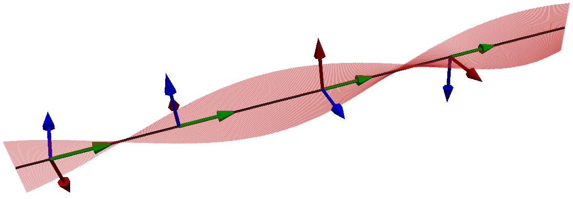
Figure 1: Unbuckled twisted ground state with $L=1$ and $M=1$. We plot the three directors $\mathbf{d}_{1}$ (red), $\mathbf{d}_{2}$ (blue) and the tangent $\mathbf{d}_{3}$ (green). Furthermore we emphasize the twist of the rod by a red ribbon which corresponds to $\mathbf{d}_{1}$.

With $\mathbf{F}=F{\bf\hat{x}}$, the rod-energy in (5) becomes

$$V[\theta,\phi,\psi]:=\int_{0}^{1}\frac{A}{2}\left(\theta_{s}^{2}+\phi_{s}^{2}\sin^{2}\theta\right)+\frac{C}{2}\left(\psi_{s}+\phi_{s}\cos\theta\right)^{2}+FL^{2}\sin\theta\cos\phi~{}ds.$$ (9)

In particular, $F>0$ corresponds to a compressive force and $F<0$ corresponds to a tensile force. It is trivial to note that the unbuckled state, represented by the following triplet of Euler angles,

$$\Theta_{0}(s)=\left(\frac{\pi}{2},0,2\pi Ms\right)$$ (10)

is a solution of the Euler-Lagrange equations in (2). We investigate the stability of $\Theta_{0}$ for three different boundary-value problems

$$\textrm{Dirichlet:}\Rightarrow\theta(0)=\theta(1)=\frac{\pi}{2}$$

$$\qquad\phi(0)=\phi(1)=0$$

$$\qquad\qquad\psi(0)=0\quad\psi(1)=2\pi M,$$ (11)

$$\textrm{Neumann:}\Rightarrow\theta_{s}(0)=\theta_{s}(1)=0$$

$$\qquad\phi_{s}(0)=\phi_{s}(1)=0$$

$$\qquad\qquad\psi(0)=0\quad\psi(1)=2\pi M,$$ (12)

and

$$\textrm{Mixed:}\Rightarrow\theta(0)=\theta(1)=\frac{\pi}{2}$$

$$\qquad\phi_{s}(0)=\phi_{s}(1)=0$$

$$\qquad\qquad\psi(0)=0\quad\psi(1)=2\pi M.$$ (13)

We first present some energy estimates that are useful for a global and local stability analysis of $\Theta_{0}$. Our first result concerns the energy difference between an arbitrary configuration of Euler angles, $\Theta=(\theta,\phi,\psi)$, and the unbuckled state, $\Theta_{0}=\left(\frac{\pi}{2},0,2\pi Ms\right)$. We can write $\Theta$ as

$$\Theta(s)=\left(\theta(s),\phi(s),\psi(s)\right)$$

$$\theta(s)=\frac{\pi}{2}+\alpha(s)\quad 0\leq s\leq 1$$

$$\phi(s)=\beta(s)\quad 0\leq s\leq 1$$

$$\psi(s)=2\pi Ms+\gamma(s)\quad\gamma(0)=\gamma(1)=0,$$ (14)

since $\psi$ is subject to Dirichlet conditions in all three boundary-value problems, (3)-(3). Further, $-\frac{\pi}{2}<\alpha<\frac{\pi}{2}$ since $\theta$ does not encounter the polar singularities by assumption. The functions, $\alpha$ and $\beta$, measure the deviation of $(\theta,\phi)$ from the unbuckled state and are not subject to any end-point constraints, since the choice of end-point constraints will depend on the choice of the boundary-value problem in (3)-(3).

From (3), it is straightforward to check that

$$\left(\psi_{s}+\phi_{s}\cos\theta\right)^{2}=4\pi^{2}M^{2}+\left(\gamma_{s}-\beta_{s}\sin\alpha\right)^{2}+4\pi M\left(\gamma_{s}-\beta_{s}\sin\alpha\right).$$ (15)

Therefore, using (3), (15) and $\gamma(0)=\gamma(1)=0$, we find that

$$2\left(V[\theta,\phi,\psi]-V\left[\frac{\pi}{2},0,2\pi Ms\right]\right)=$$

$$=\int_{0}^{1}A\left(\beta_{s}^{2}\cos^{2}\alpha+\alpha_{s}^{2}\right)+C\left(\gamma_{s}-\beta_{s}\sin\alpha\right)^{2}-4\pi MC\beta_{s}\sin\alpha+2FL^{2}\left(\cos\alpha\cos\beta-1\right)~{}ds.$$ (16)

Equation (3) is valid for all triplets of Euler angles provided they do not encounter the polar singularities. Local stability analysis requires us to only focus on small perturbations about $\Theta_{0}$. In this case, we consider perturbations, $\Theta_{\epsilon}=\left(\theta_{\epsilon},\phi_{\epsilon},\psi_{\epsilon}\right)$, where $0<{\epsilon}\ll 1$ is a small parameter and

$$\Theta_{\epsilon}(s)=\left(\theta_{\epsilon}(s),\phi_{\epsilon}(s),\psi_{\epsilon}(s)\right)$$

$$\theta_{\epsilon}(s)=\frac{\pi}{2}+{\epsilon}\alpha(s)\quad 0\leq s\leq 1$$

$$\phi_{\epsilon}(s)={\epsilon}\beta(s)\quad 0\leq s\leq 1$$

$$\psi_{\epsilon}(s)=2\pi Ms+{\epsilon}\gamma(s)\quad\gamma(0)=\gamma(1)=0,$$ (17)

for all $0\leq s\leq 1$. Then, using Taylor expansions and neglecting terms of order $\varepsilon^{3}$ and higher, (3) simplifies to

$$2\left(V[\theta_{\epsilon},\phi_{\epsilon},\psi_{\epsilon}]-V\left[\frac{\pi}{2},0,2\pi Ms\right]\right)=$$

$$={\epsilon}^{2}\int_{0}^{1}A\left(\alpha_{s}^{2}+\beta_{s}^{2}\right)+C\gamma_{s}^{2}-4\pi MC\alpha\beta_{s}-FL^{2}\left(\alpha^{2}+\beta^{2}\right)~{}ds+O(\varepsilon^{3}).$$ (18)

The second variation of the rod-energy about $\Theta_{0}$ is simply given by the right-hand side of (3) i.e. [10, 11]

$$\frac{d^{2}}{d{\epsilon}^{2}}V[\theta_{\epsilon},\phi_{\epsilon},\psi_{\epsilon}]|_{{\epsilon}=0}=\int_{0}^{1}A\left(\alpha_{s}^{2}+\beta_{s}^{2}\right)+C\gamma_{s}^{2}-4\pi MC\alpha\beta_{s}-FL^{2}\left(\alpha^{2}+\beta^{2}\right)~{}ds.$$ (19)

3.1 Dirichlet problem

We first consider the boundary-value problem (3). Then $\alpha$ and $\beta$ in (3) must vanish at the end-points. Whilst studying the static stability of $\Theta_{0}$ under Dirichlet conditions, we frequently use Wirtinger’s integral inequality cited below [17, 11].

Proposition 1

For every continuously differentiable function, $u:[0,1]\to{\mathbb{R}}$ with $u(0)=u(1)=0$, we have

$$\int_{0}^{1}\left(\frac{du}{ds}\right)^{2}~{}ds\geq\pi^{2}\int_{0}^{1}u^{2}(s)~{}ds.$$ (20)

Proposition 2

The unbuckled state, $\Theta_{0}$, has lower energy than all triplets of Euler angles, $\Theta=\left(\theta,\phi,\psi\right)$, subject to the boundary conditions in (3), provided that

$$\min_{s\in\left[0,1\right]}\cos^{2}\alpha>\frac{4MC}{A}$$ (21)

$${\rm max}\,\{FL^{2},0\}<A\pi^{2}\min_{s\in\left[0,1\right]}\cos^{2}\alpha-4\pi^{2}MC.$$

Proof: We analyze the energy difference expression in (3). Firstly, we note that

$$\cos\alpha\geq 1-\frac{\alpha^{2}}{2}$$

and hence

$$F<0\Rightarrow 2FL^{2}\left(\cos\alpha\cos\beta-1\right)>0$$

$$F>0\Rightarrow 2FL^{2}\left(\cos\alpha\cos\beta-1\right)\geq-FL^{2}\left(\alpha^{2}+\beta^{2}\right)\qquad 0\leq s\leq 1.$$ (22)

Secondly, we use Young’s inequality and ${\rm sin}^{2}\alpha\leq\alpha^{2}$ to deduce that

$$\int_{0}^{1}\beta_{s}\sin\alpha~{}ds\leq\frac{1}{\delta}\int_{0}^{1}\alpha^{2}~{}ds+\delta\int_{0}^{1}\beta_{s}^{2}~{}ds$$ (23)

for any positive real number $\delta$. We choose $\delta=\frac{1}{\pi}$, substitute (3.1) and (23) into (3) to obtain

$$2\left(V[\theta,\phi,\psi]-V\left[\frac{\pi}{2},0,2\pi Ms\right]\right)\geq$$

$$\geq\int_{0}^{1}A\left(\beta_{s}^{2}\cos^{2}\alpha+\alpha_{s}^{2}\right)-4\pi^{2}MC\alpha^{2}-4MC\beta_{s}^{2}-\max\left\{FL^{2},0\right\}\left(\alpha^{2}+\beta^{2}\right)~{}ds.$$ (24)

Using Wirtinger’s inequality (20), we easily obtain

$$2\left(V[\theta,\phi,\psi]-V\left[\frac{\pi}{2},0,2\pi Ms\right]\right)\geq$$

$$\left(A\pi^{2}\min_{s\in[0,1]}\cos^{2}\alpha-4\pi^{2}MC-\max\left\{FL^{2},0\right\}\right)\int_{0}^{1}\beta^{2}(s)~{}ds+$$

$$+\left(A\pi^{2}-4\pi^{2}MC-\max\left\{FL^{2},0\right\}\right)\int_{0}^{1}\alpha^{2}~{}ds.$$ (25)

It is clear that

$$V[\theta,\phi,\psi]-V\left[\frac{\pi}{2},0,2\pi Ms\right]>0$$

if

$$\max\left\{FL^{2},0\right\}<A\pi^{2}\min_{s\in[0,1]}\cos^{2}\alpha-4\pi^{2}MC.$$ (26)

This completes the proof of Proposition 2. $\Box$

Proposition 2 effectively tells us that $\Theta_{0}$ is the global energy minimizer, provided the twist “M” is sufficiently small compared to the material constant, $\frac{C}{A}$, and the Euler angles are bounded away from the polar singularities. Proposition 2 is a global result whereas Proposition 3 is a local stability result that is an improvement over our previous results in [10]. We recall that a rod equilibrium is stable in the static sense i.e. is a local energy minimizer, if the second variation of the rod energy is positive at the equilibrium [3, 18]. In [10], we show that $\Theta_{0}$ is stable in the static sense for forces, $F<F_{1}$, where $F_{1}$ is an explicit expression in terms of $M,C,A,L$. Correspondingly, we show that $\Theta_{0}$ is unstable for forces, $F>F_{2}$, and $F_{1}\neq F_{2}$. In Proposition 3, we close the gap between the stability and instability regimes.

Proposition 3

The unbuckled state, $\Theta_{0}$, is a local energy minimizer for terminal forces

$$FL^{2}<A\pi^{2}\left(1-\left(\frac{MC}{A}\right)^{2}\right)$$ (27)

in (9). Correspondingly, $\Theta_{0}$ is unstable for forces

$$FL^{2}>A\pi^{2}\left(1-\left(\frac{MC}{A}\right)^{2}\right).$$ (28)

Proof: An equilibrium, $\Theta^{*}=\left(\theta^{*},\phi^{*},\psi^{*}\right)$, is stable in the static sense if there exists a small neighbourhood [3, 4],

$$\Delta(\Theta)=\left\{\Theta=\left(\theta,\phi,\psi\right):|\theta-\theta^{*}|^{2}+|\phi^{*}-\phi|^{2}+|\psi^{*}-\psi|^{2}\leq{\epsilon}\right\},$$

such that

$$V[\Theta]\geq V[\Theta^{*}]\qquad\forall\Theta\in\Delta.$$

We start by looking at the second variation of the rod-energy evaluated at the unbuckled state, $\Theta_{0}$ in (19) and note that $\alpha$ and $\beta$ vanish at the end-points for the Dirichlet boundary-value problem (3). A simple integration by parts shows that $\int_{0}^{1}\alpha\beta_{s}~{}ds=-\int_{0}^{1}\beta\alpha_{s}~{}ds$ so that (19) reduces to

$$\frac{d^{2}}{d{\epsilon}^{2}}V[\theta_{\epsilon},\phi_{\epsilon},\psi_{\epsilon}]|_{{\epsilon}=0}=\int_{0}^{1}A\left(\alpha_{s}^{2}+\beta_{s}^{2}\right)+C\gamma_{s}^{2}-2\pi MC\left(\alpha\beta_{s}-\beta\alpha_{s}\right)-FL^{2}\left(\alpha^{2}+\beta^{2}\right)~{}ds.$$ (29)

We write $\alpha$ and $\beta$ as

$$\alpha=r\cos\sigma$$

$$\beta=r\sin\sigma$$ (30)

with $r^{2}=\alpha^{2}+\beta^{2}$ and $r(0)=r(1)=0$. Straightforward computations show that

$$\frac{d^{2}}{d{\epsilon}^{2}}V[\theta_{\epsilon},\phi_{\epsilon},\psi_{\epsilon}]|_{{\epsilon}=0}\geq\int_{0}^{1}A\left(r_{s}^{2}+r^{2}\sigma_{s}^{2}\right)-2\pi MCr^{2}\sigma_{s}-FL^{2}r^{2}~{}ds.$$ (31)

It suffices to note that $f(\sigma_{s})=A\sigma_{s}^{2}-2\pi MC\sigma_{s}\geq-\left(\frac{\pi MC}{A}\right)^{2}$ and the minimum is attained for $\sigma_{s}=\frac{\pi MC}{A}$. Therefore,

$$\frac{d^{2}}{d{\epsilon}^{2}}V[\theta_{\epsilon},\phi_{\epsilon},\psi_{\epsilon}]|_{{\epsilon}=0}\geq\int_{0}^{1}Ar_{s}^{2}-\left(\frac{\pi^{2}M^{2}C^{2}}{A}+FL^{2}\right)r^{2}~{}ds\geq\int_{0}^{1}\left(A\pi^{2}-\frac{\pi^{2}M^{2}C^{2}}{A}-FL^{2}\right)r^{2}~{}ds,$$ (32)

wherein we have used Wirtinger’s inequality, $\int_{0}^{1}r_{s}^{2}ds\geq\pi^{2}\int_{0}^{1}r^{2}~{}ds.$ It is clear that the second variation of the rod-energy in (19) is positive if

$$FL^{2}<A\pi^{2}\left(1-\frac{M^{2}C^{2}}{A^{2}}\right).$$

Similarly, we can show that the second variation of the rod-energy in (19), about $\Theta_{0}$, is negative for

$$FL^{2}>A\pi^{2}\left(1-\frac{M^{2}C^{2}}{A^{2}}\right),$$

by substituting

$$\alpha(s)=\sin\left(\pi s\right)\cos\left(\frac{\pi MC}{A}s\right)$$

$$\beta(s)=\sin\left(\pi s\right)\sin\left(\frac{\pi MC}{A}s\right)$$ (33)

in (LABEL:eq:17). The negativity of the second variation for a particular choice of $\left(\alpha,\beta\right)$ suffices to demonstrate the instability of $\Theta_{0}$ for forces $FL^{2}>A\pi^{2}\left(1-\frac{M^{2}C^{2}}{A^{2}}\right)$ [3, 10]. This completes the proof of Proposition 3. $\Box$

3.1.1 Bifurcations from $\Theta_{0}$

The local stability analysis in Proposition 3 relies on the integral expression for the second variation of the rod-energy in (19) and simple integral inequalities. Conjugate-point methods are an alternative and very successful approach to stability analysis; see [9, 5]. Here, we present a conjugate-point method type analysis for the unbuckled state, $\Theta_{0}$, in three dimensions and compute bifurcation diagrams for the Euler angles, $(\theta,\phi)$.

We can use integration by parts to write the second variation in (19) as

$$\frac{d^{2}}{d{\epsilon}^{2}}V[\theta_{\epsilon},\phi_{\epsilon},\psi_{\epsilon}]|_{{\epsilon}=0}=\int_{0}^{1}\left(\alpha,\beta\right)\cdot S\left(\alpha,\beta\right)~{}ds+\int_{0}^{1}C\gamma_{s}^{2}$$ (34)

where $S(\alpha,\beta)$ is a coupled system of two linear ordinary differential equations as shown below:

$$S(\alpha)=-A\alpha_{ss}-2\pi MC\beta_{s}-FL^{2}\alpha$$

$$S(\beta)=-A\beta_{ss}+2\pi MC\alpha_{s}-FL^{2}\beta.$$ (35)

From standard results in spectral theory [9], every admissible $\left(\alpha,\beta\right)$ subject to $\alpha(0)=\alpha(1)=0$ and $\beta(0)=\beta(1)=0$ can be written as a linear combination of the eigenvectors of the second-order differential operator, $S(\alpha,\beta)$, in (34). One can check that there are two families of orthogonal eigenfunctions for $(\alpha,\beta)$ given by

$$\left(\alpha,\beta\right)_{m}=\sin m\pi s\left(\cos\frac{\pi MC}{A}s,\sin\frac{\pi MC}{A}s\right)\quad m\in\mathbb{N}$$

$$\left(\alpha,\beta\right)_{m}=\sin m\pi s\left(-\sin\frac{\pi MC}{A}s,\cos\frac{\pi MC}{A}s\right)\quad m\in\mathbb{N},$$ (36)

with corresponding eigenvalues

$$\lambda_{m}=Am^{2}\pi^{2}-\frac{\pi^{2}M^{2}C^{2}}{A}-FL^{2}.$$ (37)

Equation (37) allows us to track the index or equivalently the number of negative eigenvalues as a function of the applied force and identify the critical forces

$$F_{m}=\frac{1}{L^{2}}\left(Am^{2}\pi^{2}-\frac{\pi^{2}M^{2}C^{2}}{A}\right).$$ (38)

Hence, every $(\alpha,\beta)$ can be written as

$$\left(\alpha,\beta\right)=\sum_{m=1}^{\infty}a_{m}\sin m\pi s\left(\cos\frac{\pi MC}{A}s,\sin\frac{\pi MC}{A}s\right)+\sum_{m=1}^{\infty}b_{m}\sin m\pi s\left(-\sin\frac{\pi MC}{A}s,\cos\frac{\pi MC}{A}s\right)$$ (39)

and substituting (39) into (34), we obtain

$$\frac{d^{2}}{d{\epsilon}^{2}}V[\theta_{\epsilon},\phi_{\epsilon},\psi_{\epsilon}]|_{{\epsilon}=0}=\int_{0}^{1}\left(\alpha,\beta\right)\cdot S\left(\alpha,\beta\right)~{}ds+\int_{0}^{1}C\gamma_{s}^{2}\geq$$

$$\geq\frac{1}{2}\sum_{m=1}^{\infty}\lambda_{m}\left(a_{m}^{2}+b_{m}^{2}\right).$$ (40)

From (37), it is clear that the smallest eigenvalue satisfies $\lambda_{1}>0$ for forces $FL^{2}<A\pi^{2}-\frac{\pi^{2}M^{2}C^{2}}{A}$ and thus, the second variation of the rod-energy in (19) is strictly positive for forces $FL^{2}<A\pi^{2}-\frac{\pi^{2}M^{2}C^{2}}{A}$.

In Figure 2, we plot bifurcation diagrams for the Euler angles $(\theta,\phi)$ from the trivial solution, $\Theta_{0}$, as a function of the applied load, $FL^{2}$. As can be seen from Figure 2, there is a bifurcating branch at every critical force, $F_{m}$, with $m\geq 1$, and the bifurcation diagrams are qualitatively similar to the well-known bifurcation diagrams for the polar angle, $\theta$, in two dimensions [9, 8].

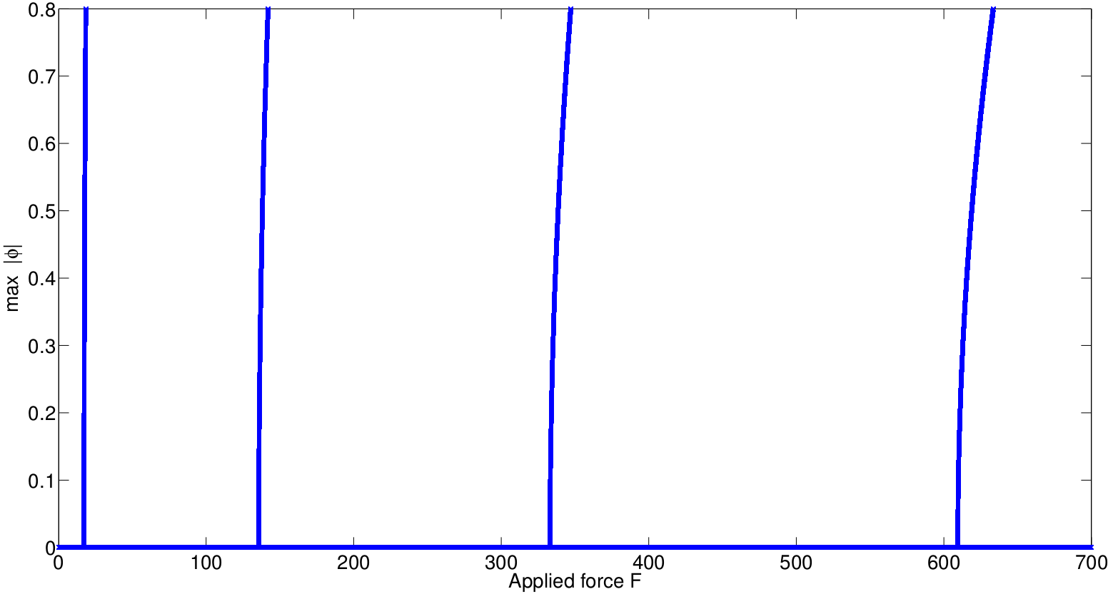
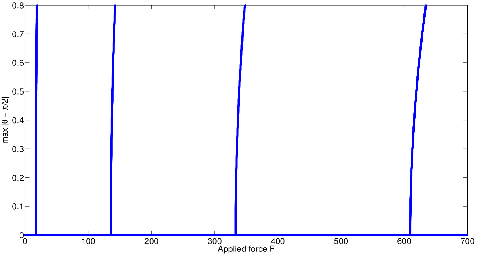
Figure 2: Bifurcation plot for $\theta$ and $\phi$ with branches at $m=1,\dots,4$. The parameter setting is $C/A=3/4$, $M=1$ and $L=1$.

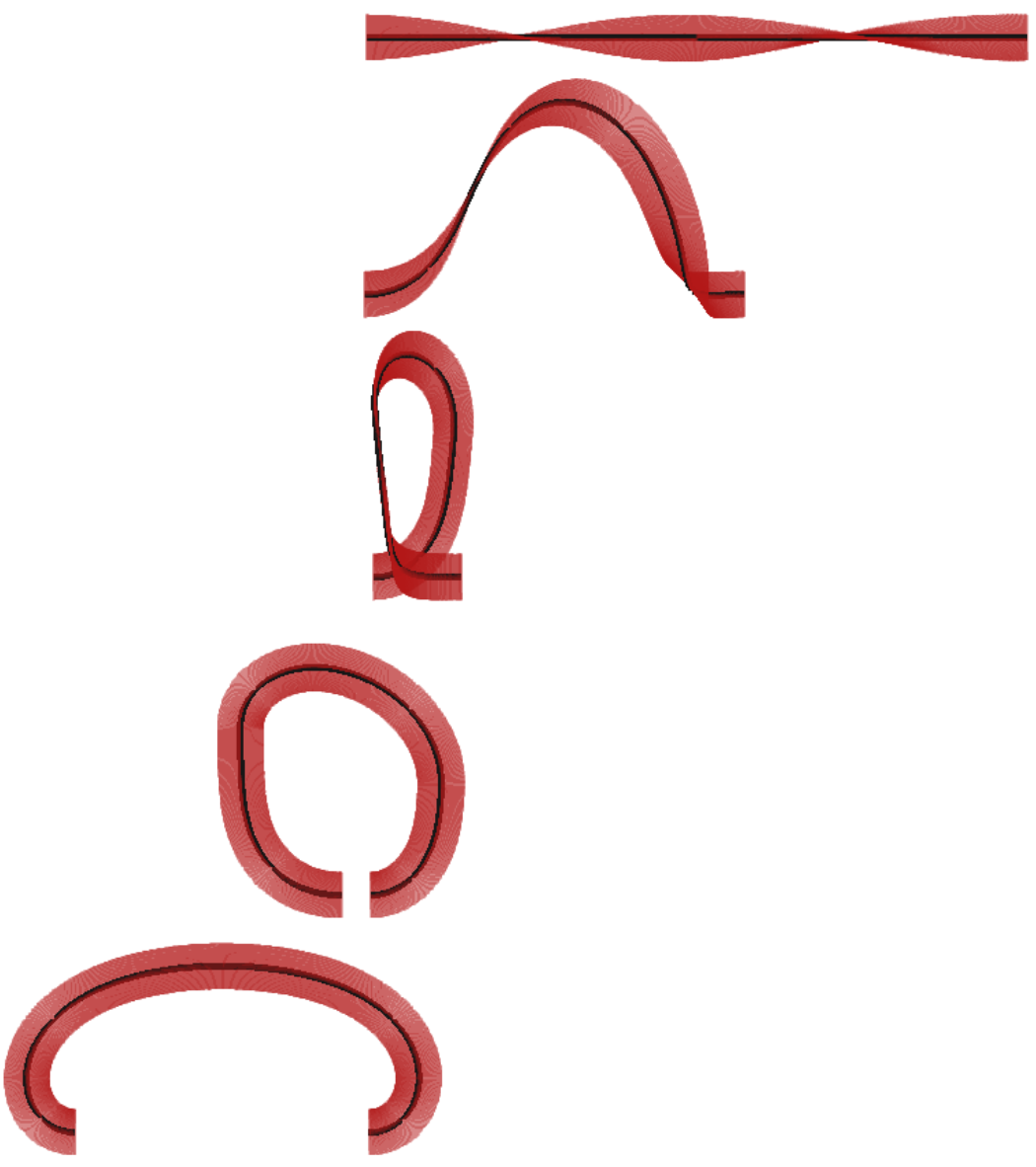
Figure 3: Evolution of the unbuckled state under a $L^{2}$-gradient flow. Parameters are $L=1$, $M=1$ and $C/A=1$. The applied force is $F=(50,0,0)$. Isoperimetric constraints ensure that $y(1)=y(0)$ and $z(0)=z(1)$.

3.1.2 Remarks on isoperimetric constraints

The local stability analysis in Section 3.1 can be generalized to the boundary-value problem (3) augmented with the following isoperimetric constraints:

$$y(0)=y(1)\Rightarrow\int_{0}^{1}\sin\theta\sin\phi~{}ds=0$$

$$z(0)=z(1)\Rightarrow\int_{0}^{1}\cos\theta~{}ds=0.$$ (41)

We consider “small” perturbations about $\Theta_{0}$ in (3), as in (3). The isoperimetric constraints (3.1.2) translate into the following integral constraints for $\alpha,\beta$ for small perturbations,

$$\int_{0}^{1}\alpha(s)ds=0$$

$$\int_{0}^{1}\beta(s)ds=0.$$ (42)

The problem of local stability analysis of $\Theta_{0}$ subject to (3.1.2) reduces to a study of the second variation of the rod-energy in (19), subject to the integral constraints (3.1.2).

Proposition 4

The unbuckled state, $\Theta_{0}$, is stable in the static sense for the boundary-value problem (3) and the isoperimetric constraints (3.1.2) for forces

$$FL^{2}<A\pi^{2}-\frac{\pi^{2}M^{2}C^{2}}{A}.$$ (43)

Correspondingly, $\Theta_{0}$ is an unstable equilibrium of the rod-energy, subject to the boundary conditions in (3) and the constraints in (3.1.2) for forces

$$FL^{2}>A\pi^{2}\left(1-\left(\frac{MC}{A}\right)^{2}\right),$$ (44)

if

$$\frac{MC}{A}=2p+1\quad p\in\mathbb{N};p\geq 1.$$ (45)

Proof: It is trivial to check that $\Theta_{0}$ satisfies the boundary conditions in (3) and the integral constraints (3.1.2). The proof of local stability for forces satisfying (43), is identical to the proof of Proposition 3. In contrast to Proposition 3, we cannot prove instability of $\Theta_{0}$ in the complementary regime with the constraints (3.1.2), for all values of $\frac{MC}{A}$.

For $\frac{MC}{A}$ satisfying (45), one can check that

$$\alpha^{*}(s)=\sin\left(\pi s\right)\cos\left(\frac{\pi MC}{A}s\right)$$

$$\beta^{*}(s)=\sin\left(\pi s\right)\sin\left(\frac{\pi MC}{A}s\right)$$ (46)

satisfy the integral constraints (3.1.2). Thus $(\alpha^{*},\beta^{*})$ qualify as an admissible perturbation that vanish at the end-points, $s=0$ and $s=1$, and satisfy the integral constraints (3.1.2). We substitute $(\alpha^{*},\beta^{*})$ into (19) with $\gamma=0$ and find that

$$\frac{d^{2}}{d{\epsilon}^{2}}V[\theta_{\epsilon},\phi_{\epsilon},\psi_{\epsilon}]|_{{\epsilon}=0}<0$$ (47)

for forces

$$FL^{2}>A\pi^{2}\left(1-\left(\frac{MC}{A}\right)^{2}\right),$$

completing the proof of Proposition 4. $\Box$

3.2 Neumann boundary conditions

We analyze the local stability of $\Theta_{0}$ subject to the Neumann conditions (3). We consider small perturbations, as in (3), and study the second variation of the rod-energy in (19),

$$\frac{d^{2}}{d{\epsilon}^{2}}V[\theta_{\epsilon},\phi_{\epsilon},\psi_{\epsilon}]|_{{\epsilon}=0}=\int_{0}^{1}A\left(\alpha_{s}^{2}+\beta_{s}^{2}\right)+C\gamma_{s}^{2}-4\pi MC\alpha\beta_{s}-FL^{2}\left(\alpha^{2}+\beta^{2}\right)~{}ds,$$ (48)

subject to

$$\alpha_{s}(0)=\alpha_{s}(1)=0$$

$$\beta_{s}(0)=\beta_{s}(1)=0.$$ (49)

Proposition 5

The unbuckled state, $\Theta_{0}$, is a locally stable equilibrium of the rod-energy in (5), subject to the boundary conditions in (3), for forces

$$FL^{2}<-4\frac{\pi^{2}M^{2}C^{2}}{A}\quad\textrm{for $A<2MC$}$$

$$FL^{2}<-2\pi^{2}MC\quad\textrm{for $A>2MC$.}$$ (50)

Proof: For $A<2MC$, we write the second variation in (19) as

$$\frac{d^{2}}{d{\epsilon}^{2}}V[\theta_{\epsilon},\phi_{\epsilon},\psi_{\epsilon}]|_{{\epsilon}=0}=\int_{0}^{1}A\left(\frac{2\pi MC}{A}\alpha-\beta_{s}\right)^{2}+C\gamma_{s}^{2}+A\alpha_{s}^{2}-FL^{2}\beta^{2}-\left(FL^{2}+\frac{4\pi^{2}M^{2}C^{2}}{A}\right)\alpha^{2}~{}ds$$ (51)

and it is clear that

$$\frac{d^{2}}{d{\epsilon}^{2}}V[\theta_{\epsilon},\phi_{\epsilon},\psi_{\epsilon}]|_{{\epsilon}=0}>0$$

for

$$FL^{2}+\frac{4\pi^{2}M^{2}C^{2}}{A}<0$$

as stated in (5).

For $A>2MC$, we write the second variation in (19) as

$$\frac{d^{2}}{d{\epsilon}^{2}}V[\theta_{\epsilon},\phi_{\epsilon},\psi_{\epsilon}]|_{{\epsilon}=0}=\int_{0}^{1}2MC\left(\pi\alpha-\beta_{s}\right)^{2}+C\gamma_{s}^{2}+A\alpha_{s}^{2}+\left(A-2MC\right)\beta_{s}^{2}-FL^{2}\beta^{2}-\left(FL^{2}+2\pi^{2}MC\right)\alpha^{2}~{}ds$$ (52)

and it is clear that $\frac{d^{2}}{d{\epsilon}^{2}}V[\theta_{\epsilon},\phi_{\epsilon},\psi_{\epsilon}]|_{{\epsilon}=0}>0$ for

$$FL^{2}+2\pi^{2}MC<0$$

as stated in (5). This completes the proof of Proposition 5. $\Box$

3.3 Mixed boundary conditions

We analyze the local stability of $\Theta_{0}$ subject to the mixed boundary conditions in (3) i.e. Dirichlet for $\theta$ and Neumann for $\phi$. We consider small perturbations, as in (3), and study the second variation of the rod-energy in (19),

$$\frac{d^{2}}{d{\epsilon}^{2}}V[\theta_{\epsilon},\phi_{\epsilon},\psi_{\epsilon}]|_{{\epsilon}=0}=\int_{0}^{1}A\left(\alpha_{s}^{2}+\beta_{s}^{2}\right)+C\gamma_{s}^{2}-4\pi MC\alpha\beta_{s}-FL^{2}\left(\alpha^{2}+\beta^{2}\right)~{}ds,$$ (53)

subject to

$$\alpha(0)=\alpha(1)=0$$

$$\beta_{s}(0)=\beta_{s}(1)=0.$$ (54)

In particular, we can use Wirtinger’s inequality for $\alpha$ i.e. $\int_{0}^{1}\alpha_{s}^{2}ds\geq\pi^{2}\int_{0}^{1}\alpha^{2}ds$. Note, that the same calculations can be done if the roles of $\alpha$ and $\beta$ in (3.3) are changed.

Proposition 6

The unbuckled state, $\Theta_{0}$, is a locally stable equilibrium of the rod-energy in (5), subject to the boundary conditions in (3), for forces

$$FL^{2}<\min\left\{\pi^{2}\left(A-\frac{4M^{2}C^{2}}{A}\right),0\right\}$$ (55)

and unstable for forces

$$FL^{2}>A\pi^{2}\frac{1-\Lambda^{2}}{1+\Lambda^{2}},$$ (56)

where $\Lambda:=\frac{2MC}{A}$. Note, that for $A=2MC$ we have a sharp result, i.e., $\Theta_{0}$ is stable for $F<0$ and unstable for $F>0$.

Proof: We write the second variation of the rod-energy about $\Theta_{0}$ as in (51).

$$\frac{d^{2}}{d{\epsilon}^{2}}V[\theta_{\epsilon},\phi_{\epsilon},\psi_{\epsilon}]|_{{\epsilon}=0}=\int_{0}^{1}A\left(\frac{2\pi MC}{A}\alpha-\beta_{s}\right)^{2}+C\gamma_{s}^{2}+A\alpha_{s}^{2}-FL^{2}\beta^{2}-\left(FL^{2}+\frac{4\pi^{2}M^{2}C^{2}}{A}\right)\alpha^{2}~{}ds\geq$$

$$\geq\int_{0}^{1}A\left(\frac{2\pi MC}{A}\alpha-\beta_{s}\right)^{2}+C\gamma_{s}^{2}-FL^{2}\beta^{2}+\left(A\pi^{2}-\left(FL^{2}+\frac{4\pi^{2}M^{2}C^{2}}{A}\right)\right)\alpha^{2}~{}ds,$$ (57)

where we have used Wirtinger’s inequality in the second step. It follows immediately from (3.3) that

$$\frac{d^{2}}{d{\epsilon}^{2}}V[\theta_{\epsilon},\phi_{\epsilon},\psi_{\epsilon}]|_{{\epsilon}=0}>0$$

if

$$FL^{2}<\min\left\{\pi^{2}\left(A-\frac{4M^{2}C^{2}}{A}\right),0\right\},$$

as stated in (55).

Similarly, we substitute

$$\alpha^{*}(s)=\sin\pi s$$

$$\beta^{*}(s)=-\frac{2MC}{A}\cos\pi s$$ (58)

into (3.3) and find that

$$\frac{d^{2}}{d{\epsilon}^{2}}V[\theta_{\epsilon},\phi_{\epsilon},\psi_{\epsilon}]|_{{\epsilon}=0}=-\frac{FL^{2}}{2}\left(1+\left(\frac{2MC}{A}\right)^{2}\right)+\frac{A\pi^{2}}{2}\left(1-\left(\frac{2MC}{A}\right)^{2}\right)$$

for this particular choice of $(\alpha^{*},\beta^{*})$. Therefore, we conclude that the second variation is negative, if

$$FL^{2}>A\pi^{2}\frac{1-\Lambda^{2}}{1+\Lambda^{2}}.$$

This completes the proof of Proposition 6. $\Box$

4 Model helices

We construct prototype helical equilibria for a naturally straight, inextensible, unshearable rod that is subject to a terminal load, $\mathbf{F}=F{\bf\hat{z}}$. This choice of terminal load is motivated by the DNA manipulation experiments reported in the literature [19]. The rod-energy is then given by

$$V[\theta,\phi,\psi]:=\int_{0}^{1}\frac{A}{2}\left(\theta_{s}^{2}+\phi_{s}^{2}\sin^{2}\theta\right)+\frac{C}{2}\left(\psi_{s}+\phi_{s}\cos\theta\right)^{2}+FL^{2}\cos\theta~{}ds,$$ (59)

where $L$ is the fixed length of the rod. The corresponding Euler-Lagrange equations are given by

$$A\theta_{ss}=A\phi_{s}^{2}\sin\theta\cos\theta-C\phi_{s}\sin\theta(\psi_{s}+\phi_{s}\cos\theta)-FL^{2}\sin\theta$$

$$\frac{d}{ds}\left[A\phi_{s}\sin^{2}\theta+C\cos\theta\left(\psi_{s}+\phi_{s}\cos\theta\right)\right]=0$$

$$\psi_{s}+\phi_{s}\cos\theta=\Gamma$$ (60)

where $\Gamma$ is a constant that depends on $\left(F,A,C\right)$.. It is straightforward to check that for given values of $\left(F,C,A,\lambda,\theta_{0}\right)$, the following family of rod configurations, $\Theta_{\lambda}=\left(\theta_{\lambda},\phi_{\lambda},\psi_{\lambda}\right)$, given by

$$\theta_{\lambda}(s)=\theta_{0}\quad 0<\theta_{0}<\pi$$

$$\phi_{\lambda}(s)=2\pi\lambda s\quad 0\leq s\leq 1$$

$$\psi_{\lambda}(s)=\left[2\pi\lambda\cos\theta_{0}\left(\frac{A}{C}-1\right)-\frac{FL^{2}}{2\pi\lambda C}\right]s+\xi$$ (61)

for any real number $\xi\in{\mathbb{R}}$, are exact solutions of the Euler-Lagrange equations (4), subject to their own boundary conditions. We take $\theta_{0}\in(0,\pi)$ so that we do not encounter the polar singularities [10, 3]. We note that the twist depends on the applied force i.e. for a given set of parameters, $\left(F,C,A,\lambda,\theta_{0}\right)$, the twist is given by

$$\psi_{s}+\phi_{s}\cos\theta=\frac{2A}{C}\pi\lambda\cos\theta_{0}-\frac{FL^{2}}{2\pi\lambda C}.$$ (62)

The solutions, $\Theta_{\lambda}$, are helices with constant curvature, $\kappa$, and constant torsion, $\eta$, given by [12]

$$\kappa=2\pi\lambda\sin\theta_{0}$$

$$\eta=2\pi\lambda\cos\theta_{0}.$$ (63)

The next step is to investigate the stability of the helical equilibria, $\Theta_{\lambda}$ in (4), subject to its own boundary conditions. For each $\lambda\in{\mathbb{R}}$ and $\theta_{0}\in(0,\pi)$, we define the following Dirichlet problem for the Euler angles:

$$\theta(0)=\theta(1)=\theta_{0}\quad 0<\theta_{0}<\pi$$

$$\phi(0)=0,\quad\phi(1)=2\pi\lambda$$

$$\psi(0)=\xi,\quad\psi(1)=2\pi\lambda\cos\theta_{0}\left(\frac{A}{C}-1\right)-\frac{FL^{2}}{2\pi\lambda C}+\xi.$$ (64)

The helical solutions, $\Theta_{\lambda}$ in (4), are equilibria of the rod-energy (59), subject to the boundary conditions (4). We compute the second variation of the rod-energy (59) about $\Theta_{\lambda}$ as shown below. We consider perturbations of the form

$$\theta_{\epsilon}(s)=\theta_{0}+{\epsilon}\alpha(s)$$

$$\phi_{\epsilon}(s)=2\pi\lambda s+{\epsilon}\beta(s)$$

$$\psi_{\epsilon}(s)=\left[2\pi\lambda\cos\theta_{0}\left(\frac{A}{C}-1\right)-\frac{FL^{2}}{2\pi\lambda C}\right]s+\xi+{\epsilon}\gamma(s)$$ (65)

with

$$\alpha(0)=\alpha(1)=0$$

$$\beta(0)=\beta(1)=0$$

$$\gamma(0)=\gamma(1)=0$$ (66)

in accordance with the imposed Dirichlet conditions for the Euler angles. One can check that

$$\frac{d^{2}}{d{\epsilon}^{2}}V[\theta_{\epsilon},\phi_{\epsilon},\psi_{\epsilon}]|_{{\epsilon}=0}=\int_{0}^{1}A\left\{\alpha_{s}^{2}+\beta_{s}^{2}\sin^{2}\theta_{0}+4\pi\lambda\alpha\beta_{s}\sin\theta_{0}\cos\theta_{0}-4\pi^{2}\lambda^{2}\alpha^{2}\sin^{2}\theta_{0}\right\}+\frac{FL^{2}}{\pi\lambda}\alpha\beta_{s}\sin\theta_{0}~{}ds+$$

$$+C\int_{0}^{1}\left(\gamma_{s}+\beta_{s}\cos\theta_{0}-2\pi\lambda\alpha\sin\theta_{0}\right)^{2}~{}ds.$$ (67)

Proposition 7

The helical solutions, defined in (4), are locally stable for

$$A>\frac{|F|L^{2}}{2\pi\lambda}$$ (68)

and for applied forces

$$\frac{|F|L^{2}}{2\pi\lambda}\left(\frac{1}{A}+\frac{4\pi^{2}\lambda^{2}}{A-\frac{|F|L^{2}}{2\pi\lambda}}\right)<\pi^{2}\left(1-4\lambda^{2}\right).$$ (69)

If $F=0$, then $\Theta_{\lambda}$ is stable for

$$-\frac{1}{2}<\lambda<\frac{1}{2}.$$ (70)

The helical solutions, defined in (4), are unstable for applied forces

$$FL^{2}\cos\theta_{0}>2A\pi^{2}\left(1-\lambda^{2}\right).$$ (71)

If $F=0$, then $\Theta_{\lambda}$ is unstable for

$$\lambda<-1\quad\lambda>1.$$ (72)

Proof: We start with the expression for the second variation in (4). We first note that

$$\int_{0}^{1}\frac{FL^{2}}{\pi\lambda}\alpha\beta_{s}\sin\theta_{0}~{}ds\geq-\frac{|F|L^{2}}{2\pi\lambda}\left\{\int_{0}^{1}\alpha^{2}~{}ds+\int_{0}^{1}\beta_{s}^{2}\sin^{2}\theta_{0}~{}ds\right\}.$$ (73)

The second variation is bounded from below by

$$\frac{d^{2}}{d{\epsilon}^{2}}V[\theta_{\epsilon},\phi_{\epsilon},\psi_{\epsilon}]|_{{\epsilon}=0}\geq\int_{0}^{1}A\left\{\alpha_{s}^{2}-4\pi^{2}\lambda^{2}\alpha^{2}\right\}-\frac{|F|L^{2}}{2\pi\lambda}\alpha^{2}~{}ds+$$

$$+\int_{0}^{1}\left(A-\frac{|F|L^{2}}{2\pi\lambda}\right)\beta_{s}^{2}\sin^{2}\theta_{0}+4\pi\lambda A\alpha\beta_{s}\sin\theta_{0}\cos\theta_{0}+4\pi^{2}\lambda^{2}A\alpha^{2}\cos^{2}\theta_{0}~{}ds.$$ (74)

It suffices to note that for $A>\frac{|F|L^{2}}{2\pi\lambda}$,

$$\left(A-\frac{|F|L^{2}}{2\pi\lambda}\right)\beta_{s}^{2}\sin^{2}\theta_{0}+4\pi\lambda A\alpha\beta_{s}\sin\theta_{0}\cos\theta_{0}+4\pi^{2}\lambda^{2}A\alpha^{2}\cos^{2}\theta_{0}=$$

$$=\left(\left(A-\frac{|F|L^{2}}{2\pi\lambda}\right)^{1/2}\beta_{s}\sin\theta_{0}+\frac{2\pi\lambda A}{\left(A-\frac{|F|L^{2}}{2\pi\lambda}\right)^{1/2}}\alpha\cos\theta_{0}\right)^{2}-\frac{2\pi A\lambda}{A-\frac{|F|L^{2}}{2\pi\lambda}}|F|L^{2}\alpha^{2}\cos^{2}\theta_{0}.$$ (75)

Then

$$\frac{d^{2}}{d{\epsilon}^{2}}V[\theta_{\epsilon},\phi_{\epsilon},\psi_{\epsilon}]|_{{\epsilon}=0}\geq$$

$$\int_{0}^{1}A\left[\alpha_{s}^{2}-4\pi^{2}\lambda^{2}\alpha^{2}-\frac{|F|L^{2}}{2\pi\lambda A}\alpha^{2}-\frac{2\pi\lambda}{A-\frac{|F|L^{2}}{2\pi\lambda}}|F|L^{2}\alpha^{2}\right]~{}ds.$$ (76)

Finally, we recall Wirtinger’s inequality

$$\int_{0}^{1}\alpha_{s}^{2}~{}ds\geq\pi^{2}\int_{0}^{1}\alpha^{2}(s)~{}ds,$$ (77)

since $\alpha$ vanishes at the end-points, $s=0$ and $s=1$. Substituting (77) into (4), we obtain

$$\frac{d^{2}}{d{\epsilon}^{2}}V[\theta_{\epsilon},\phi_{\epsilon},\psi_{\epsilon}]|_{{\epsilon}=0}\geq\int_{0}^{1}A\left[\pi^{2}-4\pi^{2}\lambda^{2}-\frac{|F|L^{2}}{2\pi\lambda A}-\frac{2\pi\lambda}{A-\frac{|F|L^{2}}{2\pi\lambda}}|F|L^{2}\right]\alpha^{2}~{}ds$$ (78)

and it is clear that

$$\frac{d^{2}}{d{\epsilon}^{2}}V[\theta_{\epsilon},\phi_{\epsilon},\psi_{\epsilon}]|_{{\epsilon}=0}>0$$

if

$$\frac{|F|L^{2}}{2\pi\lambda}\left(\frac{1}{A}+\frac{4\pi^{2}\lambda^{2}}{A-\frac{|F|L^{2}}{2\pi\lambda}}\right)<\pi^{2}\left(1-4\lambda^{2}\right).$$

This condition is clearly satified for $|F|L^{2}$ sufficiently small i.e. there exists a range of tensile and compressive forces for which the helical equilibria in (4) are stable in the static sense.

Instability result: Let

$$\alpha(s)=\sin 2\pi s$$

$$\beta(s)=\frac{\lambda\cos\theta_{0}}{\sin\theta_{0}}\left(\cos 2\pi s-1\right)$$

$$\gamma(s)=\frac{\lambda}{\sin\theta_{0}}\left(1-\cos 2\pi s\right).$$ (79)

Straightforward computations shows that

$$\beta_{s}\sin\theta_{0}+2\pi\lambda\alpha\cos\theta_{0}=0$$

$$\gamma_{s}=2\pi\lambda\frac{\alpha}{\sin\theta_{0}}=2\pi\lambda\alpha\sin\theta_{0}-\beta_{s}\cos\theta_{0}.$$ (80)

Therefore, the second variation (4), evaluated for this choice of $(\alpha,\beta,\gamma)$, is given by

$$\frac{d^{2}}{d{\epsilon}^{2}}V[\theta_{\epsilon},\phi_{\epsilon},\psi_{\epsilon}]|_{{\epsilon}=0}=\int_{0}^{1}A\left\{\alpha_{s}^{2}-4\pi^{2}\lambda^{2}\alpha^{2}\right\}-FL^{2}\cos\theta_{0}~{}ds=$$

$$=2A\pi^{2}\left(1-\lambda^{2}\right)-FL^{2}\cos\theta_{0}$$ (81)

and the second variation is negative if

$$FL^{2}\cos\theta_{0}>2A\pi^{2}\left(1-\lambda^{2}\right).$$

This completes the proof of Proposition 7. $\Box$

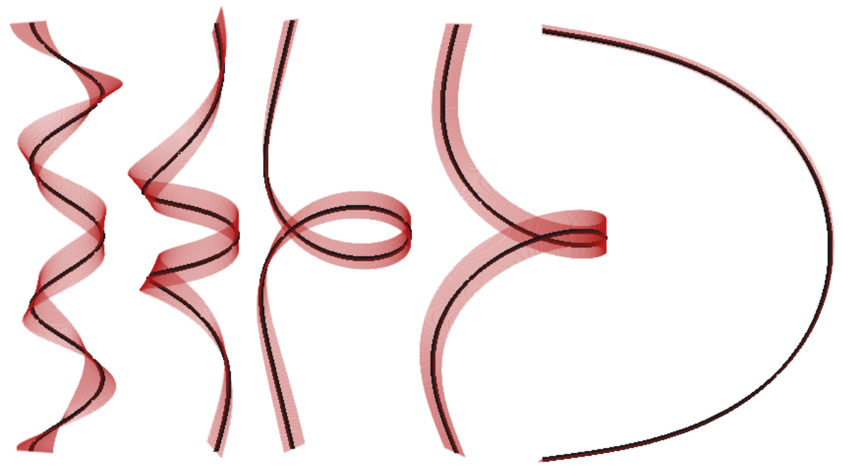
Figure 4: Evolution of an unstable helix under a $L^{2}$-gradient flow. Parameters are $L=1$, $C/A=3/4$, $\lambda=1$ and $F=0$. We have neumann boundary conditions for the Euler angles and isoperimetric constraints ensure that the endpoints of the rod stay fixed during the evolution. We note that our theory does not cover this experiment since we do not work with isoperimetric constraints.

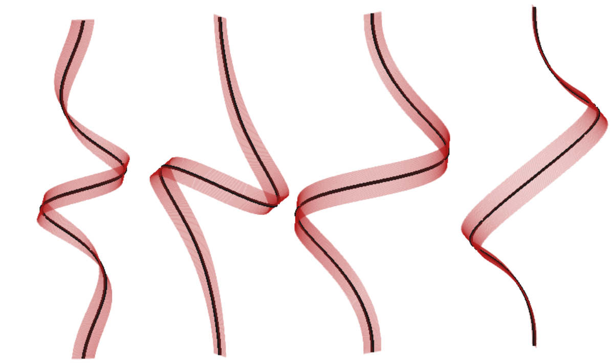
Figure 5: Evolution of an unstable helix under a $L^{2}$-gradient flow. Parameters are $L=1$, $C/A=3/4$, $\lambda=1$ and $F=0$. We have neumann boundary conditions for $\theta$ and $\phi$ and dirichlet boundary conditions for $\psi$. Furthermore, isoperimetric constraints ensure that the endpoints of the rod stay fixed during the evolution. As in Figure 4 we note, that our theory does not cover this experiment.

5 Localized buckling solutions

Next, we look at nontrivial solutions of the Euler-Lagrange equations derived in [13]. It is shown that $\Theta:\mathbb{R}\to\mathbb{R}^{3}$ defined by

$$\theta(s)={\rm arccos}\Big{(}1-\frac{2}{1+\tau^{2}}{\rm sech}^{2}(s)\Big{)}$$

$$\phi(s)={\rm arctan}\Big{(}\frac{1}{\tau}{\rm tanh}s\Big{)}+\tau s,$$

$$\psi(s)={\rm arctan}\Big{(}\frac{1}{\tau}{\rm tanh}s\Big{)}+\Big{(}3-\frac{2}{b}\Big{)}\tau s,$$

are solutions to the Euler-Lagrange equations where the force $\mathbf{F}$ is given by $\mathbf{F}=\Big{(}0,0,\frac{2}{1-z_{1}}\Big{)}$ and $z_{1}=\frac{\tau^{2}-1}{\tau^{2}+1}$. We fix a length $L$ and consider $\Theta|_{(-L,L)}:\mathbb{R}\to\mathbb{R}^{3}$ being a solution of the Euler Lagrange equation subject to it’s fulfilling boundary conditions.

For a given set of angles $U=(\zeta,\eta,\xi):\mathbb{R}\to\mathbb{R}^{3}$ we define the rod $\mathbf{r}_{U}:\mathbb{R}\to\mathbb{R}^{3}$ to be

$$\mathbf{r}_{U}(s):=\int_{0}^{s}(\sin\zeta\cos\eta,\sin\zeta\sin\eta,\cos\zeta)~{}\mbox{d}\tilde{s},$$

i.e., we solve $\frac{d\mathbf{r}_{U}}{ds}=\mathbf{d}_{3,U}$. For a set of parameters $\tau=1/2,1,2$, we will discuss numerically the stability of these localized buckling solutions. In order to compare $\Theta$ with perturbations $\Theta_{\varepsilon}$, we define the space

$$X_{\Theta}:=\{U:(-L,L)\to\mathbb{R}^{3}\,:\,r_{U}(-L)=r_{lb}(-L),r_{U}(L)=r_{lb}(L),\,\,U(-L)=\Theta(-L)\mbox{ and }U(L)=\Theta(L)\}.$$

The first variation of the rod-energy $V$ on $X_{\Theta}$, evaluated at $\Theta$ vanishes, so that we can compute a perturbation of $\Theta$ with lower energy if the second variation of $V$ on $X_{lb}$ admits a negative eigenvalue. We take the corresponding eigenfunction $U_{\Theta}$ and have that $V(\Theta+\varepsilon U_{\Theta})<V(\Theta)$ for $\varepsilon>0$ sufficiently small. This has been done numerically and the result can be seen in Figure 6.

Note, that for a perturbation $\Theta_{\varepsilon}:=\Theta+\varepsilon U_{\Theta}$ it holds $|r_{\Theta_{\varepsilon}}(L)-r_{\Theta}(L)|\sim\varepsilon^{2}$, so that $\Theta_{\varepsilon}\not\in X_{\Theta}$. That means, $\Theta_{\varepsilon}$ has lower energy but isoperimetric constraints are only satisfied up to order $\varepsilon^{2}$. In a second set of experiments we use a $L^{2}$ gradient flow as derived in Section 6 and fix the endpoints so that $r_{\Theta(t)}(L)=r_{\Theta(0)}(L)$ for $t>0$. For $\tau=1/2,1,2$ we plot the decay of energy in Figure 7 and deduce that the localizsed buckling solutions are unstable.

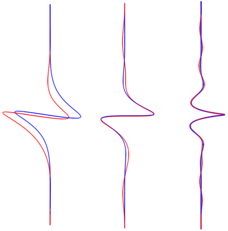
Figure 6: Local buckling solutions (blue) and perturbations with compact support (red). We set $L=10$ and $C/A=3/4$. From left to right the solutions correspond to $\tau=1/2$, $\tau=1$ and $\tau=2$. The minimal eigenvalues of the second derivative of the rod-energy was $\lambda_{min}=-106.69$,. $\lambda_{min}=-189.50$ and $\lambda_{min}=-489.80$ for the three parameters, respectively.

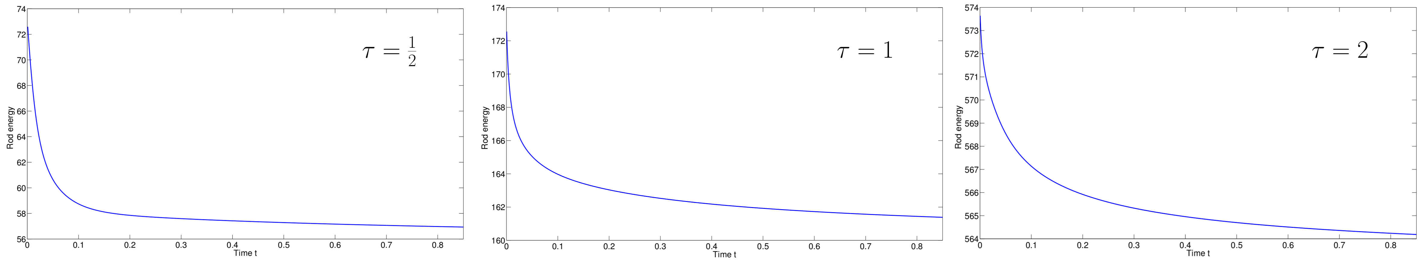
Figure 7: Evolution under a $L^{2}$ gradient flow: Initial data for the gradient flow are the local buckling solutions with parameter $\tau=\frac{1}{2},1,2$. We plot the decay of energy during the evolution with fixed endpoints and Dirichlet boundary conditions for all three angles.

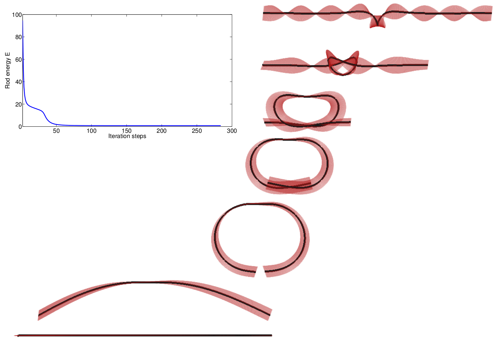
Figure 8: Evolution of a local buckling solution under the $L^{2}$-gradient flow. Parameters are $L=10$, $C/A=3/4$ and $\tau=1$. Isoperimetric constraints ensure that $x$ and $y$ components of the endpoints are fixed during the evolution. On the upper left we plot the decay of energy during the evolution.

6 Numerics

Let $I=[-L,L]$, $h=(2L)/N$ be a grid size and $(-L=s_{0},s_{1},\dots,s_{N}=L)$ a uniform partition of $I$ with nodes $s_{i}=-L+ih$, $i=0,\dots,N$, $N\in\mathbb{N}$. We define $\mathcal{S}^{1}(I)$ to be the space of piecewise affine, globally continuous functions and $\mathcal{S}_{0}^{1}(I)=\{u^{h}\in\mathcal{S}^{1}(I)\,:\,u^{h}(-L)=u^{h}(L)=0\}$. Then, every $u\in\mathcal{S}^{1}(I)$ is clearly defined by its nodal values $(u(s_{0}),\dots,u(s_{N}))$ so that we can identify $\mathcal{S}^{1}(I)$ with $\mathbb{R}^{N+1}$. The discrete energy $V^{h}:\mathbb{R}^{3(N+1)}\to\mathbb{R}$ is defined as

$$(\theta^{h},\phi^{h},\psi^{h})\mapsto\int_{0}^{1}\frac{A}{2}\left((\theta^{h}_{s})^{2}+(\phi^{h}_{s})^{2}\sin^{2}\theta^{h}\right)+\frac{C}{2}\left(\psi^{h}_{s}+\phi^{h}_{s}\cos\theta^{h}\right)^{2}+\mathbf{F}L^{2}\cdot{\bf d}_{3}^{h}~{}ds,$$

where ${\bf d}_{3}^{h}=(\sin\theta^{h}\cos\phi^{h},\sin\theta^{h}\sin\phi^{h},\cos\theta^{h})$. We can compute the first variation of $V^{h}$ in a straightforward manner,

$$\langle\delta V^{h}(\Theta^{h}),(\alpha^{h},\beta^{h},\gamma^{h})\rangle=\frac{\mbox{d}}{\mbox{d}\epsilon}|_{\epsilon=0}V^{h}(\theta^{h}+\epsilon\alpha^{h},\phi^{h}+\epsilon\beta^{h},\psi^{h}+\epsilon\gamma^{h}).$$

The semi-discrete in space $L^{2}$-gradient flow is then defined as

$$\Big{(}\partial_{t}\Theta^{h},(\alpha^{h},\beta^{h},\gamma^{h})\Big{)}_{L^{2}}=-\langle\delta V^{h}(\Theta^{h}),(\alpha^{h},\beta^{h},\gamma^{h})\rangle,$$

where $(u,v)_{L^{2}}=\int_{-L}^{L}u\cdot v\mbox{d}s$ is the standard $L^{2}$-inner product. Given a time step size $\kappa>0$ we define the time steps $t_{j}=\kappa j$. An implicite time-discretization of the $L^{2}$-gradient flow leads to a family of angles $(\Theta_{j}^{h})_{j\in\mathbb{N}}$ related to the time step $t_{j}$. Given $\Theta_{j}^{h}\in\mathbb{R}^{3(N+1)}$, the angles at time $t_{j}$, we compute the discrete velocity $d_{t}\Theta^{h}_{j}$ as a solution of

$$\Big{(}d_{t}\Theta^{h}_{j},(\alpha^{h},\beta^{h},\gamma^{h})\Big{)}=-\langle\delta V^{h}(\Theta^{h}_{j}+\kappa d_{t}\Theta^{h}_{j}),(\alpha^{h},\beta^{h},\gamma^{h})\rangle,$$

and update $\Theta^{h}_{j+1}=\Theta^{h}_{j}+\kappa d_{t}\Theta^{h}_{j}$.

6.1 Isoperimetric Constraints

We now introduce a method for the conservation of isoperimetric constraints during the evolution. The idea goes back to [20, 21] where it was used to ensure conservation of area and mass of biomembranes during a similar energy minimization procedure. We will focus on the constraint

$$x(0)=x(1),\quad\mbox{i.e.}\quad\int_{-L}^{L}{\rm sin}\,\theta\,{\rm cos}\,\phi\,\mbox{d}s=0,$$

and note, that adding more side conditions is straightforward. We introduce the extended energy

$$W^{h}(\Theta^{h})=V^{h}(\Theta^{h})+\lambda\left(\int_{-L}^{L}{\rm sin}\,\theta^{h}\,{\rm cos}\,\phi^{h}\,\mbox{d}s\right).$$

and compute the first variation with respect to $\Theta^{h}$

$$\langle\delta W^{h}(\Theta^{h}),(\alpha^{h},\beta^{h},\gamma^{h})\rangle=\langle\delta V^{h}(\Theta^{h}),(\alpha^{h},\beta^{h},\gamma^{h})\rangle+\lambda\left(\int_{-L}^{L}\left(\alpha^{h}{\rm cos}\,\theta^{h}\,{\rm cos}\,\phi^{h}-\beta^{h}{\rm cos}\,\theta^{h}\,{\rm sin}\,\phi^{h}\right)\,\mbox{d}s\right).$$

Following [20] we compute in each time-step the velocities $v_{V^{h}}$ and $v_{Iso}$ via

$$\Big{(}v_{V^{h}},(\alpha^{h},\beta^{h},\gamma^{h})\Big{)}=-\langle\delta V^{h}(\Theta^{h}),(\alpha^{h},\beta^{h},\gamma^{h})\rangle,$$

and

$$\Big{(}v_{Iso},(\alpha^{h},\beta^{h},\gamma^{h})\Big{)}=-\int_{-L}^{L}\left(\alpha^{h}{\rm cos}\,\theta^{h}\,{\rm cos}\,\phi^{h}-\beta^{h}{\rm cos}\,\theta^{h}\,{\rm sin}\,\phi^{h}\right)\,\mbox{d}s$$

and define the function

$$\rho_{j}(\lambda)=\int_{-L}^{L}{\rm sin}\,\theta^{h}(\lambda)\,{\rm cos}\,\phi^{h}(\lambda)\,\mbox{d}s,$$

where $\Theta(\lambda)=\Theta^{h}_{j}+\kappa(v_{V^{h}}+\lambda v_{Iso})$. Now, we use a Newton iteration to compute a solution $\lambda_{j}$ of $\rho^{j}(\lambda)=0$ and set $\Theta^{h}_{j+1}=\Theta^{h}_{j}+\kappa\left(v_{V^{h}}+\lambda_{j}v_{Iso}\right)$.

Fully discrete gradient flow with constraints. Given a tolerance $TOL>0$, a grid size $h>0$ and a partition of $[-L,L]$, we start with an initial set of angles $\Theta_{0}^{h}$ and time-step size $\kappa>0$. We set $j:=0$ and iterate on $j$ the following steps:

• Compute $v_{V^{h}},v_{Iso}\in[\mathcal{S}_{0}^{1}(\mathcal{T})]^{3}$ satisfying

  $$\Big{(}v_{V^{h}},(\alpha^{h},\beta^{h},\gamma^{h})\Big{)}=-\langle\delta V^{h}(\Theta^{h}),(\alpha^{h},\beta^{h},\gamma^{h})\rangle,$$

  and

  $$\Big{(}v_{Iso},(\alpha^{h},\beta^{h},\gamma^{h})\Big{)}=-\int_{-L}^{L}\left(\alpha^{h}{\rm cos}\,\theta^{h}\,{\rm cos}\,\phi^{h}-\beta^{h}{\rm cos}\,\theta^{h}\,{\rm sin}\,\phi^{h}\right)\,\mbox{d}s,$$

  for all $(\alpha^{h},\beta^{h},\gamma^{h})\in[\mathcal{S}^{1}_{0}(\mathcal{T})]^{3}$.

• Compute a solution $\lambda_{j}$ of $\rho^{j}(\lambda)=0$ and set $\Theta^{h}_{j+1}=\Theta^{h}_{j}+\kappa\left(v_{V^{h}}+\lambda_{j}v_{Iso}\right)$.

• Stop if ${\rm res}^{j}=\left|V^{h}(\Theta^{h}_{j+1})-V^{h}(\Theta^{h}_{j})\right|<TOL$. Otherwise set $j=j+1$ and go to (1).

7 Conclusions

In this paper, we study three different types of rod equilibria, including both trivial and buckled solutions, in a fully 3D setting with different types of boundary conditions and isoperimetric constraints. The analytic methods in Section 3 and Section 4 are relatively explicit and transparent, only depending on integral inequalities. These methods yield explicit stability estimates in terms of the twist, load and elastic constants and give valuable information about the incipient instabilities, as illustrated in Section 3.1.1. In particular, we bypass the traditional problems with Neumann boundary conditions in Section 3.2. The numerical experiments in Sections 4 and 5 could be carried out systematically to devise model conditions under which these non-trivial solutions could be stabilized. The work in this paper is only foundational for 3D studies of rod equilibria and there are several open directions e.g. dynamical studies of the fully nonlinear Kirchhoff rod equations, inclusion of intrinsic curvature into the stability analysis, non-equilibria transitions between different equilibria as a function of the external load and the role of external loads in stabilization and destabilization effects. However, the analytic methods in this paper can be carried over to more complicated situations of extensible-shearable rods or rods with intrinsic curvature and the numerical methods can be readily adapted to include topological and various boundary constraints. Therefore, we believe that these methods provide new tools and approaches to applied mathematicians in this area and we hope to report on new 3D effects in future work.

Acknowledgments:

AM and AR thank Alain Goriely for several helpful discussions and suggestions, which led to the improvement of this manuscript. AM and AR also thank John Maddocks, Sebastien Neukrich and Gert van der Heijden for helpful comments. AM is supported by an EPSRC Career Acceleration Fellowship EP/J001686/1, an OCCAM Visiting Fellowship and a Keble Research Grant. AR is supported by KAUST, Award No. KUK-C1-013-04 and the John Fell OUP fund.

References

[1]
D. J. Lee, R. Cortini, A. P. Korte, E. L. Starostin, G. H. M. van der Heijden,
and A. A. Kornyshev.
Chiral effects in dual-dna braiding.
Soft Matter, pages –, 2013.
[2]
A. Goriely, M. Nizette, and M. Tabor.
On the dynamics of elastic strips.
J. Nonlinear Sci., 11(1):3–45, 2001.
[3]
J. H. Maddocks.
Stability of nonlinearly elastic rods.
Arch. Rational Mech. Anal., 85(4):311–354, 1984.
[4]
R. E. Caflisch and J. H. Maddocks.
Nonlinear dynamical theory of the elastica.
Proc. Roy. Soc. Edinburgh Sect. A, 99(1-2):1–23, 1984.
[5]
K. A. Hoffman.
Methods for determining stability in continuum elastic-rod models of
DNA.
Philos. Trans. R. Soc. Lond. Ser. A Math. Phys. Eng. Sci.,
362(1820):1301–1315, 2004.
[6]
S. Neukirch and M. E. Henderson.
Classification of the spatial equilibria of the clamped elastica:
Numerical continuation of the solution set.
International Journal of Bifurcation and Chaos,
14(04):1223–1239, 2004.
[7]
O. M. O′ Reilly and D. M. Peters.
On stability analyses of three classical buckling problems for the
elastic strut.
Journal of Elasticity, 105(1-2):117–136, 2011.
[8]
R. S. Manning.
Conjugate points revisited and Neumann-Neumann problems.
SIAM Rev., 51(1):193–212, 2009.
[9]
R. S. Manning.
A catalogue of stable equilibria of planar extensible or inextensible
elastic rods for all possible dirichlet boundary conditions.
Journal of Elasticity, pages 1–26, 2013.
[10]
A. Majumdar, C. Prior, and A. Goriely.
Stability estimates for a twisted rod under terminal loads: a
three-dimensional study.
J. Elasticity, 109(1):75–93, 2012.
[11]
A. Majumdar and A. Goriely.
Static and dynamic stability results for a class of three-dimensional
configurations of Kirchhoff elastic rods.
Phys. D, 253:91–101, 2013.
[12]
N. Chouaieb, A. Goriely, and J. H. Maddocks.
Helices.
Proceedings of the National Academy of Sciences,
103(25):9398–9403, 2006.
[13]
M. Nizette and A. Goriely.
Towards a classification of Euler-Kirchhoff filaments.
J. Math. Phys., 40(6):2830–2866, 1999.
[14]
S. S. Antman and C. S. Kenney.
Large buckled states of nonlinearly elastic rods under torsion,
thrust, and gravity.
Arch. Rational Mech. Anal., 76(4):289–338, 1981.
[15]
S. Antman.
Nonlinear Problems of Elasticity.
Applied mathematical sciences. Springer, 2006.
[16]
N. Chouaieb and J. H. Maddocks.
Kirchhoff’s problem of helical equilibria of uniform rods.
Journal of Elasticity, 77(3):221–247, 2004.
[17]
B. Dacorogna.
Direct methods in the calculus of variations, volume 78 of Applied Mathematical Sciences.
Springer, New York, second edition, 2008.
[18]
M. R. Hestenes.
Calculus of variations and optimal control theory.
Robert E. Krieger Publishing Co. Inc., Huntington, N.Y., 1980.
Corrected reprint of the 1966 original.
[19]
B. Fain, J. Rudnick, and S. Östlund.
Conformations of linear dna.
Phys. Rev. E, 55:7364–7368, Jun 1997.
[20]
A. Bonito, R. H. Nochetto, and M. S. Pauletti.
Parametric FEM for geometric biomembranes.
Comput. Phys., 229:3171–3188, 2010.
[21]
S. Bartels, G. Dolzmann, R. H. Nochetto, and A. Raisch.
Finite element methods for director fields on flexible surfaces.
Interfaces Free Bound., 14(2):231–272, 2012.