Higgs Phenomenology in the Two-Singlet Model

Abstract

We study the phenomenology of the Standard Model (SM) Higgs sector extended by two singlet scalars. The model predicts two CP-even scalars $h_{1,2}$ which are a mixture of doublet and singlet components as well as a pure singlet scalar $S_{0}$ which is a dark matter candidate. We show that the model can satisfy the relic density and direct detection constraints as well as all the recent ATLAS and CMS measurements. We also discuss the effect of the extra Higgs bosons on the different Higgs triple couplings $h_{i}h_{j}h_{k}$, $i,j,k=1,2$. A particular attention is given to the triple self-coupling of the SM-like Higgs where we found that the one loop corrections can reach 150% is some cases. We also discuss some production mechanisms for $h_{1}$ and $h_{2}$ at the LHC as well as at the future International Linear Collider. It is found that the production cross section of a pair of SM-like Higgs bosons could be much larger than the corresponding one in the SM and would reveal physics beyond the SM if observable. We also show that in this model the branching ratio of the SM-like Higgs decaying to two singlet scalars could be of the order of 20%, therefore the production of the SM Higgs followed by its decay to a pair of singlets would be an important source of production of singlet scalars.

1 Introduction

The Large Hadron Collider (LHC) at CERN has just successfully finished its first phase of operation with a 7 and 8 TeV run. Both experiments ATLAS and CMS at the LHC announced last July the discovery of a Higgs-like particle with a mass in the range 125-126 GeV ATLAS ; CMS . Both collaborations, ATLAS and CMS reported a clear excess in the two photon channel and in the $ZZ^{\ast}$ channel ATLAS ; CMS . The discovery is also confirmed with less significance in other channels atlasmoriond ; cmsmoriond , like $WW^{\ast}$ which has a lower mass resolution, and also by the final Tevatron results reported by CDF and D0 experiments tevatron .

The extraction of the couplings of the Higgs-like particle to gauge bosons and fermions achieved up to now from the $7\oplus 8$ TeV data shows that this particle looks more and more like the SM Higgs boson atlasmoriond ; cmsmoriond , while more data is needed in order to fully pin down the exact nature of the newly discovered particle.

Although, ATLAS and CMS data show no significant deviation of the signal from the SM predictions. At ATLAS, the diphoton channel shows some small enhancement. The overall signal strength for diphoton is about $1.55_{-0.28}^{+0.33}$, which corresponds to about 2 $\sigma$ deviation from the SM prediction ATLAS2G ; while the other channels are consistent with the SM. However, at CMS, the new analysis for diphoton mode based on multivariate analysis CMS2G gives $0.77\pm 0.27$, which is compatible with the SM. Many models beyond the SM have been proposed to explain the diphoton excess, but the actual disagreement between ATLAS and CMS does not allow to extract significant conclusions.

Since the Higgs-like particle decays to two photons, it can not be spin one particle because of the Young Landau theorem, it is either spin-0 or spin-2. Recently, spin and parity of the Higgs-like particle were studied from the angular distribution of the diphoton, $ZZ^{\ast}$ and $WW^{\ast}$ decay channels atlaspin ; cmspin at ATLAS and CMS. Both collaborations disfavor the pure pseudoscalar hypothesis $J^{P}=0^{-}$; and also a pure spin-2 hypothesis. In addition, the spin one hypotheses is also disfavored with an even higher confidence.

Therefore, the first phase of the LHC run is just the beginning of a precise measurement program that starts with $7\oplus 8$ TeV data and will be completed with the second run of the LHC at 13-14 TeV as well as by the International Linear Collider (ILC). It is well known that the precise measurement programs at the ILC and the LHC are complementary Weiglein:2004hn ; Peskin:2012we . Such measurements, if accurate enough, can be also helpful in discriminating between models through their sensitivity to radiative correction effects, in particular in specific cases like the decoupling limit. It is well known that many SM extensions such as SUSY models or extended Higgs sector models possess such decoupling limit where the light Higgs boson completely mimics the SM Higgs.

ATLAS and CMS discovery, has lead to several phenomenological constraints on the scalar sector in such extensions of SM Higgs sector with extra doublets, Higgs sector with doublet and singlets, or Higgs sector with doublet and triplets etc… The fact that the Higgs-like particle couplings to gauge bosons and fermions are consistent with the SM predictions; can put severe constraints on all beyond SM extensions that try to accommodate such Higgs-like particle.

The aim of this paper is to study the phenomenology of the SM Higgs sector extended by two real, spinless and $\mathbb{Z}_{2}$ symmetric fields which can explain the Dark Matter (DM) TSM ; last . The model has three CP-even scalars, two of which, $h_{1,2}$, are mixing of a $SU(2)_{L}$ doublet and a singlet, whereas a $\mathbb{Z}_{2}$-odd singlet $S_{0}$ remains unmixed, which can play the role of DM candidate. However, both $h_{1}$ and $h_{2}$ can decay to a pair of $S_{0}$, if kinematically allowed, it will contribute to the invisible decay of $h_{1}$ or $h_{2}$; and will potentially modify the properties of the Higgs-like particle $h_{1}$ or $h_{2}$. In addition, the annihilation of $S_{0}$ into SM particles will provide thermal relic density and the scattering of $S_{0}$ on nucleons will lead to direct detection signatures.

In the light of the recent discovery of a 125 GeV Higgs-like particle ATLAS ; CMS , we investigate, in the framework of the two singlets model, the possibility that one of the scalars $h_{1}$ or $h_{2}$ is the particle observed by ATLAS and CMS. Therefore, we consider the two cases where one of the scalar eigenmasses $m_{1}$ or $m_{2}$ lies in the range 123.5-127.5 GeV tolerated by ATLAS and CMS experimental results, with their couplings to the SM fermions and gauge bosons close to the SM case, i.e., $g_{h_{i}f\bar{f}}^{2}/g_{hf\bar{f}}^{2(SM)}=g_{h_{i}VV}^{2}/g_{hVV}^{2(SM)}\geq 0.9$. Then, we will investigate the phenomenology of the non SM-like Higgs in both cases.

This paper is organized as follows. We first introduce the two singlet model and its theoretical constraints in the second section. We investigate the DM and its direct detection constraints on the two singlet model in the third section. Section IV is devoted to various Higgs triple self-couplings that exist in this model with particular attention given to the triple self-coupling of the SM-like Higgs scalar. We discuss some phenomenological aspects of the model such as the Higgs decays and double Higgs production in section V and present our conclusion in section VI. In the appendices, we give the tree-level cubic and quartic scalar couplings and we provide the details of the calculation of the effective Higgs triple couplings from the effective potential.

2 The Two-Singlet Model

In this model, we extend the Standard Model with two real scalar fields $S_{0}$ and $\chi_{1}$; which transform under the discrete symmetry $\mathbb{Z}_{2}^{(0)}\otimes\mathbb{Z}_{2}^{(1)}$ as

$$\begin{array}[c]{ccc}\mathbb{Z}_{2}^{(0)}:&&(S_{0},\chi_{1})\rightarrow(-S_{0},\chi_{1})\\ \mathbb{Z}_{2}^{(1)}:&&(S_{0},\chi_{1})\rightarrow(S_{0},-\chi_{1}).\end{array}$$ (1)

The field $\chi_{1}$ has a non vanishing vacuum expectation value, which breaks $\mathbb{Z}_{2}^{(1)}$ spontaneously, whereas, $\left\langle S_{0}\right\rangle=0$; and hence, $S_{0}$ is a dark matter candidate. Both fields are standard model gauge singlets and hence can interact with ’visible’ particles only via the Higgs doublet $H$. The part of the Lagrangian that includes the fields $S_{0}$, $H$, and $\chi_{1}$ is written as follows:

$$\mathcal{L}=\left(D_{\mu}H\right)^{{\dagger}}D_{\mu}H+\frac{1}{2}\left(\partial_{\mu}S_{0}\right)+\frac{1}{2}\left(\partial_{\mu}\chi_{1}\right)-V(H,\chi_{1},S_{0}),$$ (2)

with

$$H^{T} =\left(h^{+},~{}~{}(\upsilon+\widetilde{h}+i\chi_{0})/\sqrt{2}\right),~{}D_{\mu}H=\left(\partial_{\mu}-ig_{2}/2\sigma^{a}W_{\mu}^{a}-ig_{1}/2B_{\mu}\right)H,$$

$$\chi_{1} =\upsilon_{1}+\widetilde{\chi}_{1},$$ (3)

where $\sigma^{a}$ are the Pauli matrices, $W_{\mu}^{a}$ ($B_{\mu}$) and $g_{2}$ ($g_{1}$) are the $SU(2)_{L}$ ($U(1)_{Y}$) gauge field and coupling, respectively. The tree-level scalar potential that respects the $\mathbb{Z}_{2}$ symmetries is given by TSM

$$V(H,\chi_{1},S_{0}) =-\mu^{2}H^{{\dagger}}H+\frac{\lambda}{6}\left(H^{{\dagger}}H\right)^{2}+\frac{\widetilde{m}_{0}^{2}}{2}S_{0}^{2}-\frac{\mu_{1}^{2}}{2}\chi_{1}^{2}+\frac{\eta_{0}}{24}S_{0}^{4}+\frac{\eta_{1}}{24}\chi_{1}^{4}$$

$$+\frac{\lambda_{0}}{2}S_{0}^{2}H^{{\dagger}}H+\frac{\lambda_{1}}{2}\chi_{1}^{2}H^{{\dagger}}H+\frac{\eta_{01}}{4}S_{0}^{2}\chi_{1}^{2}.$$ (4)

The parameters $\mu^{2}$ and $\mu_{1}^{2}$ could be eliminated from the potential by imposing ($\upsilon,\upsilon_{1}$) to be the absolute minimum as

$$\mu^{2} =\lambda\upsilon^{2}/6+\lambda_{1}\upsilon_{1}^{2}/2+\tfrac{1}{\upsilon}\left.\tfrac{\partial}{\partial\tilde{h}}V^{1-l}\right|_{\tilde{h}=\upsilon,\chi_{1}=\upsilon_{1},S_{0}=0.},$$

$$\mu_{1}^{2} =\eta_{1}\upsilon_{1}^{2}/6+\lambda_{1}\upsilon^{2}/2+\tfrac{1}{\upsilon_{1}}\left.\tfrac{\partial}{\partial\chi_{1}}V^{1-l}\right|_{\tilde{h}=\upsilon,\chi_{1}=\upsilon_{1},S_{0}=0.},$$ (5)

where $V^{1-l}$ is the one-loop corrections to the scalar potential. While the condition

$$\widetilde{m}_{0}^{2}+\lambda_{0}\upsilon^{2}/2+\eta_{01}\upsilon_{1}^{2}/2+\left.\tfrac{1}{S_{0}}\tfrac{\partial}{\partial S_{0}}V^{1-l}\right|_{\widetilde{h}=\upsilon,\chi_{1}=\upsilon_{1},S_{0}=0.}>0,$$ (6)

should be fulfilled in order that the potential does not develop a vev in the direction of $S_{0}$. In fact, the conditions (6) are not enough to guaranty the vacuum being ($\upsilon,\upsilon_{1}$); one must require that the Jacobian must be positive, which is equivalent to the fact that the two mass-squared eigenvalues are positive. In addition, we impose the vacuum stability condition

$$\allowbreak\lambda\eta_{0}\eta_{1}-9\eta_{0}\lambda_{1}^{2}-9\lambda\eta_{01}^{2}-9\eta_{1}\lambda_{0}^{2}+54\lambda_{0}\lambda_{1}\eta_{01}>0,$$ (7)

where $\lambda$, $\eta_{1}$ and $\eta_{0}$ must be strictly positive, while $\lambda_{0}$, $\lambda_{1}$ and $\eta_{01}$ could have negative values within the condition (7). Moreover, $\lambda$, $\eta_{1}$ $\eta_{0}$, $\lambda_{0}$, $\lambda_{1}$ and $\eta_{01}$ must remain perturbative.

The spontaneous breaking of the electroweak and the $\mathbb{Z}_{2}$ symmetries introduces the two vacuum expectation values $\upsilon$ and $\upsilon_{1}$ respectively. With the value of $\upsilon$ being fixed experimentally to 246 GeV from W gauge boson mass, the model has ten parameters. The minimization conditions of the effective potential allows one to eliminate $\mu^{2}$ and $\mu_{1}^{2}$ in favor of $(\upsilon,\upsilon_{1})$. Then, we are left with eight parameters: $\lambda$, $\lambda_{0}$, $\lambda_{1}$, $\eta_{0}$, $\eta_{1}$, $\eta_{01}$, $\upsilon_{1}$ and $m_{0}$. However, the DM self-coupling constant $\eta_{0}$ does not enter the calculations of the lowest-order processes of this work, so effectively, we are left with seven input parameters.

The physical Higgs scalars $h_{1}$ and $h_{2}$, with masses $m_{1}$ and $m_{2}$ (with $m_{1}<m_{2}$), are related to the excitations of the neutral component of the SM Higgs doublet field, Re$(H^{(0)})=(\upsilon+{\widetilde{h}})\sqrt{2}$, and the field $\chi_{1}=\widetilde{\chi}_{1}+\upsilon_{1}$ through a mixing angle $\theta$. The scalars $\widetilde{h}$ and $\widetilde{\chi}_{1}$ are not the interacting fields but components of the eigenstates $h_{1}$ and $h_{2}$ which are obtained after the electroweak and the $\mathbb{Z}_{2}$ symmetries are spontaneously broken. Then the interactions of the DM candidate with the scalar sector that is relevant to the relic density, are not these in (4), but instead, their modification

$$\left(\begin{array}[c]{c}h_{1}\\ h_{2}\end{array}\right)=\left(\begin{array}[c]{cc}\cos\theta&\sin\theta\\ -\sin\theta&\cos\theta\end{array}\right)\left(\begin{array}[c]{c}\widetilde{h}\\ \widetilde{\chi}_{1}\end{array}\right),$$ (8)

as shown in (9). In our work, the CP-even scalar masses and the mixing angle are estimated at one-loop. Here the quartic interactions get modified and new cubic interactions emerge TSM . The couplings of the $h_{1}$ and $h_{2}$ with fermions and gauge fields are just the projections of the doublets couplings using (8). The scalar potential that emerges after the electroweak symmetry breaking is given as a function of scalar eigenstates by

$$V(h_{1},h_{2},S_{0}) =\frac{m_{0}^{2}}{2}S_{0}^{2}+\frac{m_{1}^{2}}{2}h_{1}^{2}+\frac{m_{2}^{2}}{2}h_{2}^{2}$$

$$+\frac{\lambda_{001}^{(3)}}{2}S_{0}^{2}h_{1}+\frac{\lambda_{002}^{(3)}}{2}S_{0}^{2}h_{2}+\frac{\lambda_{111}^{(3)}}{6}h_{1}^{3}+\frac{\lambda_{222}^{(3)}}{6}h_{2}^{3}+\frac{\lambda_{112}^{(3)}}{2}h_{1}^{2}h_{2}+\frac{\lambda_{122}^{(3)}}{2}h_{1}h_{2}^{2}$$

$$+\frac{\eta_{0}}{24}S_{0}^{4}+\frac{\lambda_{1111}^{(4)}}{24}h_{1}^{4}+\frac{\lambda_{2222}^{(4)}}{24}h_{2}^{4}+\frac{\lambda_{0011}^{(4)}}{4}S_{0}^{2}h_{1}^{2}+\frac{\lambda_{0022}^{(4)}}{4}S_{0}^{2}h_{2}^{2}+\frac{\lambda_{0012}^{(4)}}{2}S_{0}^{2}h_{1}h_{2}$$

$$+\frac{\lambda_{1112}^{(4)}}{6}h_{1}^{3}h_{2}+\frac{\lambda_{1122}^{(4)}}{4}h_{1}^{2}h_{2}^{2}+\frac{\lambda_{1222}^{(4)}}{6}h_{1}h_{2}^{3},$$ (9)

where the triple and quartic coupling are given in appendix A. In our analysis we require that:

• all the dimensionless quartic couplings to be $\ll 4\pi$ for the theory to remain perturbative,

• they have to be chosen in such a way that the ground state stability is insured;

• and we assume that the DM mass lies up to 1 TeV.

In our work, we consider the following values for the free parameters;

$$\lambda,\eta_{0},\eta_{1},\left|\lambda_{0}\right|,\left|\lambda_{1}\right|,\left|\eta_{01}\right|<3$$

$$20<\frac{\upsilon_{1}}{\mathrm{GeV}}<2000,~{}1<\frac{m_{0}}{\mathrm{GeV}}<1000,$$ (10)

and we make random choices taking into account the value of the relic density lying in the physical interval (13) and being not in conflict with direct detection DM experiments. Also, one of the CP even scalars mass lies around 123.5-127.5 $\mathrm{GeV}$, with couplings to SM fermions and gauge bosons that are similar to the SM by more than $\epsilon\gtrsim$ 90%, where $\epsilon$ is $\cos^{2}\theta$ or $\sin^{2}\theta$ depending if $h_{1}$ or $h_{2}$ is the SM-like Higgs, respectively.

For our numerical illustration, we define the following two scenarios: A and B where the SM-like Higgs is $h_{1}$ and $h_{2}$ respectively. In addition, the invisible decay channel in case A $h_{1}\rightarrow 2DM$ could be open up to 20%, while both $h_{2}\rightarrow 2DM$ and $h_{2}\rightarrow h_{1}h_{1}$ should not exceed together 20% in case B. In fact, the former constraint on the invisible decay originates from global fit analysis to ATLAS and CMS data global ; global0 ; strumia . When deriving this limit in a global analysis, it is assumed that the Higgs boson has similar couplings to fermions and gauge bosons as in the SM and additional invisible decay modes. For instance, if the effective gluon-gluon-Higgs, $\gamma$-$\gamma$-Higgs or Higgs couplings to fermions are considered, the Higgs couplings to gauge bosons are modified, and therefore the above limit could be exceeded global0 ; strumia . Therefore, in our work, we consider the conservative choice $B(h\rightarrow invisible)\leq 20\%$. Recently, both ATLAS and CMS have searched for invisible decay of the Higgs. Assuming the Higgs-strahlung SM cross section for $pp\rightarrow ZH$ with 125 GeV SM Higgs boson, ATLAS exclude with 95% confidence level an invisible branching fraction of the Higgs larger than 65% and CMS obtain similar result Higgs-invisible . CMS also looks for invisible decay of the Higgs through vector boson fusion process and exclude an invisible branching fraction of the Higgs larger than 69% CMS-VBF . When data from $pp\rightarrow ZH$ and VBF are combined the limit becomes 54% CMS-VBF .

In our numerical scans, we will consider the parameter values that:

• ensure that one CP-even scalar is the SM-like by more than 90%,

• give the right amount of the DM relic density,

• do not conflict the direct detection DM experiments such as CDMSII CDMSII and Xe100 Xe ,

• in case A, the heavy scalar $h_{2}$ escapes the ATLAS ATLAS and CMS CMS bounds; and in case B, the light Higgs escapes the LEP constraints OPAL ;

• and the invisible SM-like Higgs decay channel should not exceed 20%.

3 Dark Matter & Detection

In the framework of the thermal dynamics of the Universe within the standard cosmological model kolb , the WIMP relic density is related to its annihilation rate by the familiar relation:

$$\Omega_{D}\bar{h}^{2}=\frac{1.07\times 10^{9}x_{f}}{\sqrt{g_{\ast}}m_{Pl}\left\langle\upsilon_{12}\sigma_{ann}\right\rangle\mathrm{GeV}},$$ (11)

with

$$x_{f}=\ln\frac{0.038~{}m_{Pl}m_{0}\left\langle\upsilon_{12}\sigma_{ann}\right\rangle}{\sqrt{g_{\ast}x_{f}}}.$$ (12)

The notations are as follows: the quantity $\bar{h}$ is the Hubble constant in units of 100 $km\times s^{-1}\times Mpc^{-1}$, the quantity $m_{Pl}=1.22\times 10^{19}$ GeV the Planck mass, $m_{0}$ the DM mass, $x_{f}=m_{0}/T_{f}$ the ratio of the DM mass to the freeze-out temperature $T_{f}$ and $g_{\ast}$ the number of relativistic degrees of freedom with mass less than $T_{f}$. The quantity $\left\langle\upsilon_{12}\sigma_{ann}\right\rangle$ is the thermally averaged annihilation cross section of a pair of two DM particles multiplied by their relative velocity in the center-of-mass reference frame TSM . When considering the current value for the DM relic density DM

$$\Omega_{D}\bar{h}^{2}=0.1187\pm 0.0017;$$ (13)

and taking the approximate values of $x_{f}\approx 19.2\sim 21.6$ and $m_{0}\approx 10\sim 100$ $\mathrm{GeV}$, we get

$$\left\langle\upsilon_{12}\sigma_{ann}\right\rangle=(1.9\pm 0.2)\times 10^{-9}\text{ }\mathrm{GeV}^{-2}.$$ (14)

The value in (14) for the DM annihilation cross section translates into a relation between the parameters of a given theory entering the calculated expression of $\left\langle\upsilon_{12}\sigma_{ann}\right\rangle$, hence imposing a constraint on these parameters will limit some of the possible range of DM masses. These constraints can be exploited to examine aspects of the theory like perturbativity, while at the same time reducing the number of parameters by one. However, since we will consider a wide range for the DM mass, $1\sim 1000$ $\mathrm{GeV}$, the ratio $x_{f}$ will be estimated numerically using (11), especially for small mass values. Depending on how heavy/light is the DM candidate, its main annihilation channel will be to fermion pairs $f\bar{f}$ ($b\bar{b}$, $c\bar{c}$, $\tau\bar{\tau}$, or $\mu\bar{\mu}$), but for very large mass values, the channels $h_{1}h_{1}$, $h_{1}h_{2}$, $h_{2}h_{2}$, $WW$, $WW^{\ast}$, $ZZ$, $ZZ^{\ast}$ and $t\bar{t}$ could be also important. All the explicit formula of the annihilation cross section are given in TSM .

During previous years, experiments such as CDMS II CDMSII , XENON 10/100 Xe and CoGeNT CoGe have been searching for signal of elastic scattering of a DM WIMP off nucleon targets in deep underground. Although, no unambiguous signal has been seen yet, they yielded increasingly stringent exclusion bounds on the DM-nucleon elastic scattering total cross section $\sigma_{det}$ in terms of the DM mass $m_{0}$. The direct detection cross section for the scattering of $S_{0}$ (the DM candidate in this model) off nucleon, $\sigma_{det}$, is given by TSM ; last

$$\sigma_{det}=\frac{g_{HNN}^{2}m_{N}^{2}}{4\pi(m_{N}+m_{0})^{2}}\left[\frac{\lambda_{001}^{(3)}\cos\theta}{m_{1}^{2}}-\frac{\lambda_{002}^{(3)}\sin\theta}{m_{2}^{2}}\right]^{2},$$ (15)

where $m_{N}$ is the nucleon mass, $\lambda_{00i}^{(3)}$ is the coupling constants of $h_{i}S_{0}^{2}$ given in appendix A, and $g_{HNN}$ is the effective Higgs-nucleon coupling, which is estimated based on heavy baryon chiral perturbation theory to be $g_{HNN}\simeq 1.5\times 10^{-3}~{}$SVZ ; Ch ; GLS , whereas lattice calculations give somehow smaller values Lat1 ; Lat2 .

In our work, the free parameters are chosen in such a way that the spectrum of the scalar sector has a SM Higgs like particle of 125 GeV, and the relic density of $S_{0}$ is consistent with the Planck data DM . As it is shown in Fig. 1, we find that for most of the benchmarks, the elastic scattering cross section $\sigma_{det}$ is below $10^{-45}$ $cm^{2}$, i.e., below all the experimental bounds including the new one from Xe100 as well the latest LUX results LUX , especially for DM masses larger than 125 GeV for case A; and 50 GeV for case B.

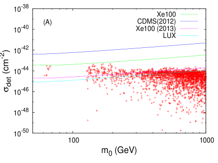
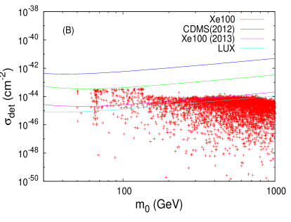
Figure 1: The direct detection cross section versus the DM mass compared to the recent Xe100 and LUX results, where the left and right panels correspond to the cases A and B respectively. It is clear that all the considered benchmarks are not in conflict with previous experimental bounds such as Xe100 (2012) and CDMSII (2012).

This behavior could be due to the cancelation between the two terms inside the bracket in Eq. (15) or/and to the scaling of $\sigma_{det}$ as the inverse square of $m_{0}$ which results in the suppression of the heavy DM event rate. However, for DM lighter than $30$ GeV, the invisible Higgs decay fraction exceeds $20\%$, and so it is in conflict with ATLAS and CMS data.

4 The Triple Higgs Coupling

With the discovery of the Higgs-like particle at ATLAS and CMS with a mass in the range 125-126 GeV, and in order to establish the Higgs mechanism for the electroweak symmetry breaking we need to measure not only Higgs couplings to fermions and gauge bosons but also the triple and quartic self-coupling of the Higgs boson which are necessary for Higgs potential reconstruction. The measurement of the triple and quartic couplings, if precise enough, can help distinguishing between various SM extensions. The Triple Higgs self-coupling can be, in principle, measured directly in pair-production of Higgs boson at the LHC with high luminosity option double1 and/or at $e^{+}e^{-}$ International Linear Collider Weiglein:2004hn .
At the LHC, it is rather difficult to reconstruct the triple coupling of the Higgs because of the smallness of the cross section $gg\rightarrow hh$ as well as the large associated QCD background. Several parton level analysis have been devoted to this process with the following final states: $hh\rightarrow W^{+}W^{-}W^{+}W^{-}$ (which would lead to same sign leptons) double2 , $hh\rightarrow b\bar{b}W^{+}W^{-}$ double0 , $hh\rightarrow b\bar{b}\gamma\gamma$ double3 and $hh\rightarrow b\bar{b}\tau^{+}\tau^{-}$ double0 . The last two processes seem to be very promising for High luminosity at the LHC. The authors in ref. Dolan:2012rv used the recent jet substructure techniques to study the Higgs pair production and the Higgs pair production in association with hard jet, where it is found that $b\bar{b}\tau^{+}\tau^{-}$ and $b\bar{b}\tau^{+}\tau^{-}+jet$ channels can be used to constrain the Triple Higgs self-coupling in the SM.

On the other hand, at the ILC, the process $e^{+}e^{-}\rightarrow Zhh\rightarrow l^{+}l^{-}b\bar{b}b\bar{b}$ has been investigated with 500 GeV center of mass energy with 1 ab^-1 luminosity and it turns out that this process can be useful for measuring the Higgs self-coupling at the ILC Weiglein:2004hn .

In our study, the Triple Higgs self-couplings are estimated by taking the third derivatives of the effective potential at one-loop using the exact formulae given in appendix B, where we show how the renormalization scale disappears in favor of measured quantities. In our model, the deviation of the Triple Higgs self-coupling from the SM value can not come only from the modification of Higgs couplings to top quarks through the reduction factor $\epsilon$ (see Eq. (37)), but also comes from new contributions of the other Higgs scalar and the DM candidate. In the rest of this section, for both cases A and B, we estimate the magnitude of different scalar triple couplings at one-loop and their deviation from the SM value. In what follows, the renormalization scale is taken to be the Higgs mass 125 GeV.

Case A: $h_{1}$ SM-like

In this case, $h_{1}$ is the SM-like while $h_{2}$ is dominated by singlet component. The relevant Triple Higgs self-couplings are $\lambda_{h_{1}h_{1}h_{1}}$, $\lambda_{h_{1}h_{1}h_{2}}$ and $\lambda_{h_{1}h_{2}h_{2}}$, where the first one corresponds to $\lambda_{hhh}$ in the SM case. The other two couplings $\lambda_{h_{1}h_{1}h_{2}}$ and $\lambda_{h_{1}h_{2}h_{2}}$ have at least one $h_{1}$ leg which could give access to an associate production $h_{2}h_{1}$ or double production $h_{2}h_{2}$ through: $pp\rightarrow h_{1}^{\ast}\rightarrow h_{1}h_{2}$, $pp\rightarrow h_{1}^{\ast}\rightarrow h_{2}h_{2}$ at the LHC or $e^{+}e^{-}\rightarrow Zh_{1}^{\ast}\rightarrow Zh_{1}h_{2}$, $e^{+}e^{-}\rightarrow Zh_{1}^{\ast}\rightarrow Zh_{2}h_{2}$ at the ILC.

In order to illustrate the magnitude of the one-loop corrected triple Higgs couplings, we show in Fig. 2-left the triple SM-like Higgs coupling versus its tree-level value. It is clear that only the coupling $\lambda_{h_{1}h_{1}h_{1}}$ which receives significant corrections at the one-loop level and make it larger than its corresponding tree level value. Also one has to mention that its value is the smallest one with respect to the other ones: $\lambda_{h_{1}h_{2}h_{2}}$ and $\lambda_{h_{1}h_{1}h_{2}}$. Note that the value of $\lambda_{h_{2}h_{2}h_{2}}$ (which is not shown here) could be much larger than the others, i.e. up to $\lambda_{h_{2}h_{2}h_{2}}\sim 8\times\upsilon$.

In order to show the effect of these new contributions on this triple coupling $\lambda_{h_{1}h_{1}h_{1}}$, we define the following quantity $\Delta_{h_{1}h_{1}h_{1}}=(\lambda_{h_{1}h_{1}h_{1}}-\lambda_{hhh}^{SM})/\lambda_{hhh}^{SM}$, which represents the relative enhancement on the triple Higgs coupling at one-loop with respect to the same quantity estimated at one-loop in the SM for the recently measured Higgs mass.

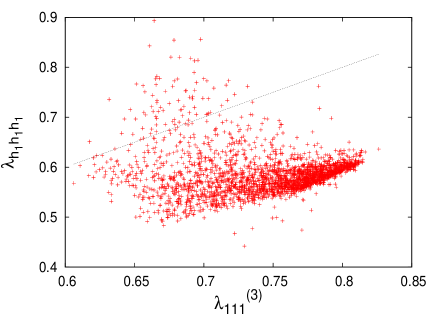
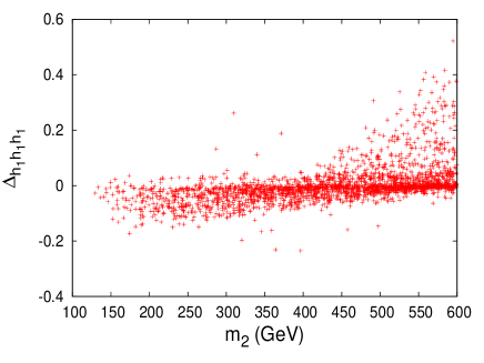
Figure 2: Left panel: the SM-like triple Higgs coupling versus its tree-level value in units of the EW vev value for randomly chosen sets of parameters, where the SM-like Higgs is defined according to case A. Right panel: the relative enhancement on the SM-like triple Higgs coupling of with respect to the SM value versus the mass of the heavy scalar $m_{2}$ for the same sets of parameters.

In Fig. 2-right, we show $\Delta_{h_{1}h_{1}h_{1}}$ as a function of the heavy scalar mass $m_{2}$. It is clear that in this case, the one-loop corrections to the SM-like Higgs $h_{1}$ could have an enhancement greater than 40%. Since we have subtracted the SM contribution at one-loop, this enhancement is then attributed to the new contributions of $h_{2}$ and $S_{0}$.

Case B: $h_{2}$ SM-like

In the case where $h_{2}$ is SM-like, $h_{1}$ is dominated by singlet component and according to our convention is lighter than $h_{2}$. In this case, the relevant triple Higgs coupling is $\lambda_{h_{2}h_{2}h_{2}}$, which corresponds to $\lambda_{hhh}$ in the SM case. Like in case A, the other two couplings $\lambda_{h_{1}h_{2}h_{2}}$ and $\lambda_{h_{1}h_{1}h_{2}}$ have at least one $h_{2}$ leg which could give access to an associate production $h_{2}h_{1}$ or double production $h_{1}h_{1}$ through the processes: $pp\rightarrow h_{2}^{\ast}\rightarrow h_{1}h_{2}$, $pp\rightarrow h_{2}^{\ast}\rightarrow h_{1}h_{1}$ at the LHC or $e^{+}e^{-}\rightarrow Zh_{2}^{\ast}\rightarrow Zh_{1}h_{2}$, $e^{+}e^{-}\rightarrow Zh_{2}^{\ast}\rightarrow Zh_{1}h_{1}$ at an $e^{+}e^{-}$ machine. Fig. 3-left shows the one-loop correction effects to the SM-like triple coupling versus its tree-level value.

In this case, the one-loop corrections to the coupling $\lambda_{h_{2}h_{2}h_{2}}$ make it larger than its corresponding tree level value. In Fig. 3-right, we plot the quantity $\Delta_{h_{2}h_{2}h_{2}}=(\lambda_{h_{2}h_{2}h_{2}}-\lambda_{hhh}^{SM})/{\lambda_{hhh}^{SM}}$ as a function of the light scalar mass $m_{1}$.

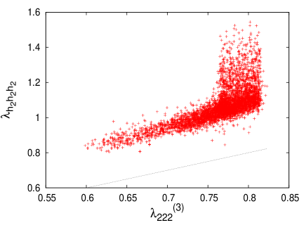
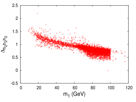
Figure 3: Left panel: the triple Higgs couplings in absolute values, in units of the EW vev value, versus its tree-level value for randomly chosen sets of parameters, where the SM-like Higgs is defined according to case B. Right panel: the relative enhancement on the SM-like Triple Higgs coupling of $h_{2}$ with respect to the SM case versus the mass of the light scalar $m_{1}$ for randomly chosen sets of parameters.

We see that in this case, the one-loop corrections to the SM-like Higgs $h_{2}$ could enjoy large enhancement which lies between few 40% and 100% for $10~{}\mathrm{GeV}<m_{1}<100~{}\mathrm{GeV}$. This effect is even amplified and can reach 150% and more when we cross the threshold $h_{2}\rightarrow h_{1}h_{1}$ region. This kind of large radiative corrections have been also reported in the framework of two Higgs doublet model Kanemura:2004mg .

5 Higgs Phenomenology

In this section, we will discuss $h_{1}$ and $h_{2}$ phenomenology.

5.1 Higgs Decays

The partial decay widths of the two Higgs scalars $h_{1,2}$ into SM particles such as $f\bar{f}$, $WW$ ($WW^{\ast}$) and $ZZ$ ($ZZ^{\ast}$) is just the SM rate multiplied by $\epsilon=\cos^{2}\theta,\sin^{2}\theta$, depending on whether $h_{1}$ or $h_{2}$ is the decaying particle. This $\epsilon$ factor apply also for loop mediated process such as $h_{i}\rightarrow\gamma\gamma,Z\gamma,gg$. The decay rate of $h_{2}\rightarrow h_{1}h_{1}$ is given by

$$\Gamma\left(h_{2}\rightarrow h_{1}h_{1}\right)=\frac{\left(\lambda_{112}^{(3)}\right)^{2}}{32\pi m_{2}}\left(1-\frac{4m_{1}^{2}}{m_{2}^{2}}\right)^{\frac{1}{2}}\Theta\left(m_{2}-2m_{1}\right),$$ (16)

and the light/heavy Higgs decay to DM final state $S_{0}$ is

$$\Gamma\left(h_{i}\rightarrow S_{0}S_{0}\right)=\frac{\left(\lambda_{00i}^{(3)}\right)^{2}}{32\pi m_{i}}\left(1-\frac{4m_{0}^{2}}{m_{i}^{2}}\right)^{\frac{1}{2}}\Theta\left(m_{i}-2m_{0}\right).$$ (17)

Moreover, in this model $h_{2}$ can also decay to Triple Higgs $h_{1}$ if kinematically allowed: $h_{2}\rightarrow h_{1}h_{1}h_{1}$ which would require $m_{2}>3m_{1}$. This decay channel has three contributions: quartic term $h_{2}h_{1}h_{1}h_{1}$, contribution mediated by off-shell $h_{1}^{\ast}$: $h_{2}\rightarrow h_{1}h_{1}^{\ast}\rightarrow h_{1}h_{1}h_{1}$ and a contribution mediated by off-shell $h_{2}^{\ast}$: $h_{2}\rightarrow h_{1}h_{2}^{\ast}\rightarrow h_{1}h_{1}h_{1}$. This decay, even if it is open could not compete with the 2 body phase space decay $h_{2}\rightarrow h_{1}h_{1}$ due to the 3 body phase space suppression.

The reduction factor for the SM final state process $h_{1}\rightarrow X_{SM}$ is given by

$$R_{X_{SM}}\left(h_{1}\right) =G\frac{B(h_{1}\rightarrow X_{SM})}{B^{SM}(h\rightarrow X_{SM})}$$

$$=\frac{c^{4}\Gamma_{tot}^{SM}\left(h_{1}\right)}{c^{2}\Gamma_{tot}^{SM}\left(h_{1}\right)+\Gamma(h_{1}\rightarrow S_{0}S_{0})},$$ (18)

with the G-factor is given by

$$G=\frac{\sigma(gg\rightarrow h_{1})}{\sigma^{SM}(gg\rightarrow h)}=c^{2}.$$ (19)

The reduction factor for $h_{2}\rightarrow X_{SM}$ is

$$R_{X_{SM}}\left(h_{2}\right)=\frac{s^{4}\Gamma_{tot}^{SM}\left(h_{2}\right)}{s^{2}\Gamma_{tot}^{SM}\left(h_{2}\right)+\Gamma(h_{2}\rightarrow X_{NSM})},$$ (20)

where $X_{NSM}$ denotes all the non SM final states such as $h_{1}h_{1}$, $h_{1}h_{1}h_{1}$, $S_{0}S_{0}$ or $h_{1}S_{0}S_{0}$. For case B, due to the fact that $R_{X_{SM}}\left(h_{2}\right)$ is proportional to $s^{2}$, all values of $s^{2}<0.1$ will be in perfect agreement with ATLAS and CMS data.

In the following plots, we will show our numerical results illustrating different physical quantities for the case A previously introduced where $h_{1}$ is the SM-like Higgs.

Figure 4: Left panel: the branching ratios of the decay channels $h_{2}\rightarrow t\bar{t},~{}h_{2}\rightarrow h_{1}h_{1}$ and $h_{2}\rightarrow S_{0}S_{0}$ versus its mass. Right panel: the branching ratio of the heavy Higgs to the SM particles final states versus the heavy Higgs mass; scaled by the same quantities evaluated in the SM.

In Fig. 4, we show the branching ratios of $h_{2}$-decay to SM (right) and non-SM (left) final states. In Fig. 4(left), we illustrate the branching ratio of the heavy Higgs $h_{2}$ into $t\bar{t}$, $S_{0}S_{0}$ and $h_{1}h_{1}$ as a function of $m_{2}$. It is clear that for $m_{2}\approx 125-150$ GeV, $h_{2}$ will decay dominantly to SM particles such as $b\bar{b}$, $WW^{\ast}$ and $ZZ^{\ast}$, if the decay $h_{2}\rightarrow S_{0}S_{0}$ is kinematically forbidden. Once $h_{2}\rightarrow S_{0}S_{0}$ is open, it dominates all the other decays. For the range $m_{2}\approx 150-250$ GeV, we can see the opening of the three body phase space channel $h_{2}\rightarrow h_{1}h_{1}^{\ast}\rightarrow h_{1}f\bar{f}$ which is rather small (less than $10^{-4}$). However, once $m_{2}\geq 250$ GeV the on-shell decay $h_{2}\rightarrow h_{1}h_{1}$ is open and compete with $h_{2}\rightarrow S_{0}S_{0}$. As one can see, the channels $h_{2}\rightarrow h_{1}h_{1}$ and $h_{2}\rightarrow t\bar{t}$ can reach 40% and 10% branching ratio respectively.

As a summary, if the invisible channel $h_{2}\rightarrow S_{0}S_{0}$ does not dominate, one can say that:

• for $m_{\mathbf{2}}<250$ GeV, $h_{\mathbf{2}}$ Higgs decays similar to the SM case,

• for 250 GeV $<m_{\mathbf{2}}<400$ GeV, it decays similar to the SM by 60% and to $h_{\mathbf{1}}h_{\mathbf{1}}$ by 40 %;

• for $m_{\mathbf{2}}>400$ GeV, $B(h_{2}\rightarrow h_{1}h_{1})$ becomes 30% and $B(h_{2}\rightarrow t\bar{t})$ becomes important as 10%.

At the end, we give the total decay width for the two CP-even scalars in both cases in Fig. 5. It is well known that the SM Higgs with a mass of 125 GeV has a very narrow width which is $\Gamma_{h}\approx 4$ MeV.

In case A where $h_{1}$ is the SM-like, the total width of $h_{1}$ is in the range 3.7-4.6 MeV while the total width of $h_{2}$ can be located between $10^{-3}$ and $10^{4}$ MeV. A very narrow width of $h_{2}$ means that Higgs to Higgs decays of $h_{2}$ such that $h_{2}\rightarrow h_{1}h_{1}$ and $h_{2}\rightarrow S_{0}S_{0}$ are closed and only $h_{2}$ decays to SM particles are open which are suppressed because $h_{2}$ is dominated by singlet.

In case B where $h_{2}$ is the SM-like, its total width is very narrow (3.5-4.6 MeV) if $h_{2}\rightarrow S_{0}S_{0}$ and $h_{2}\rightarrow h_{1}h_{1}$ are closed. Once these two channels are open, the total width of $h_{2}$ grows up to 5.7 MeV. The total width of $h_{1}$ which is dominated by singlet is rather small, less than 0.2 MeV.

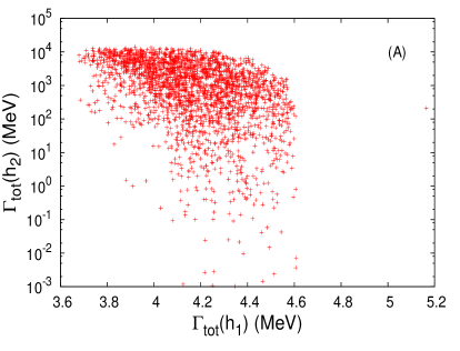
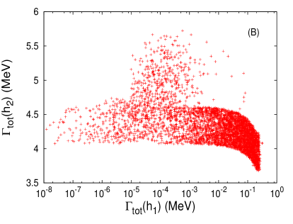
Figure 5: The total decay width of the SM-like Higgs versus the non SM-like Higgs in both cases A (left) and B (right).

For some benchmarks in both cases, the decay $h_{2}\rightarrow h_{1}h_{1}h_{1}$ is kinematically possible, and it is important to estimate how large is this branching ratio. In Fig. 6, we show $B(h_{2}\rightarrow h_{1}h_{1}h_{1})$ versus $m_{2}$ ($m_{1}$) for case A (B).

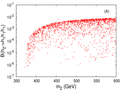
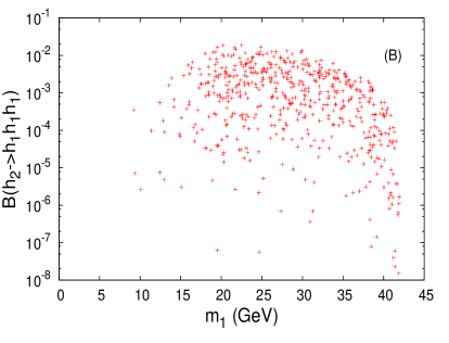
Figure 6: The branching ratio B($h_{2}\rightarrow h_{1}h_{1}h_{1}$) versus the non SM-like Higgs mass for both cases A (up-left) and B (up-right).

It is clear that this branching ratio is in the order of $\mathcal{O}(10^{-2})$ and below. We stress here that in case where $h_{2}$ is the SM-like Higgs boson, which has quite substantial cross section, it may be possible to measure such 3-body phase space decay with a branching ratio of the order $10^{-2}$.

For case B, we show in Fig. 7 the branching ratio for $h_{2}\rightarrow h_{1}h_{1}$ (including $h_{2}\rightarrow h_{1}h_{1}^{\ast}$) versus the light Higgs mass; and the resonant production cross section of both $gg\rightarrow h_{2}\rightarrow h_{1}h_{1}$ and $gg\rightarrow h_{2}\rightarrow h_{1}h_{1}h_{1}$ versus the light Higgs mass is shown in Fig. 8.

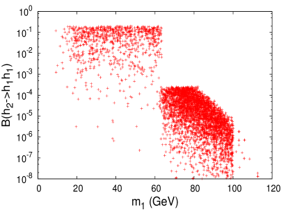
Figure 7: The branching ratio B($h_{2}\rightarrow h_{1}h_{1}$) versus the non SM-like Higgs mass for case B.

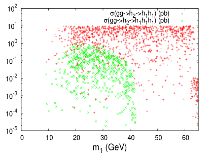
Figure 8: The resonant production cross section for double and triple singlet $h_{1}$ as a function of $m_{1}$ for case B. The red points are for $\sigma(gg\to h_{2})\times B(h_{2}\to h_{1}h_{1})$, and the green ones are for $\sigma(gg\to h_{2})\times B(h_{2}\to h_{1}h_{1}h_{1})$, all cross sections are in pb.

5.2 Higgs Production

Same as in the SM, at the LHC the dominant production cross section for the SM like Higgs $h_{1}$ or $h_{2}$ would be dominated by gluon fusion process which is mediated by the top loops. The cross section rate for a single Higgs production will be simply modified by the mixing angle $c^{2}$ or $s^{2}$ depending on $h_{1}$ or $h_{2}$ production:

$$\sigma(gg\rightarrow h_{1})=c^{2}\times\sigma(gg\rightarrow h_{SM})\quad,\quad\sigma(gg\rightarrow h_{2})=s^{2}\times\sigma(gg\rightarrow h_{SM})$$

$$\sigma(pp\rightarrow Vh_{1})=c^{2}\times\sigma(pp\rightarrow Vh_{SM})\quad,\quad\sigma(pp\rightarrow Vh_{2})=s^{2}\times\sigma(pp\rightarrow Vh_{SM})$$ (21)

It is clear that in case A where $h_{1}$ is the SM-like and dominated by doublet component $c\approx 1$ and $h_{2}$ is dominated by singlet component. In this case, the cross section $\sigma(gg\rightarrow h_{1})$ (or $\sigma(pp\rightarrow Vh_{1})$) will be typically close to SM one while $\sigma(gg\rightarrow h_{2})$ (or$\ \sigma(pp\rightarrow Vh_{2})$) will be suppressed by $s^{2}$ which is rather small in this case. Same thing apply for the case B.

For the double Higgs production which is a good probe for Triple Higgs self-coupling, we will evaluate $gg\rightarrow h_{i}h_{j}$ for the LHC and $e^{+}e^{-}\rightarrow Zh_{i}h_{j}$ for the ILC in some benchmark scenarios which are given in Table-1 and Table-2. We remind here that in the SM, the double Higgs production at the LHC $gg\rightarrow hh$ proceeds at one-loop level trough vertex and boxes contributions (top exchange) which interfere destructively in the total cross section. In the two singlets model under consideration, the vertex contributions can be mediated by the 2 Higgs scalars $h_{1,2}$: $gg\rightarrow h_{1,2}^{\ast}\rightarrow h_{i}h_{j}$ which could give some resonant effects from $h_{2}\rightarrow h_{1}h_{1}$.

5.2.1 Resonant Production of the SM-like Higgs

In case A, where $h_{1}$ is the SM-like Higgs and $h_{2}$ is dominated by singlet component. In this case the processes $gg\rightarrow h_{1}^{\ast},h_{2}^{\ast}\rightarrow h_{1}h_{1}$ or $e^{+}e^{-}\rightarrow Zh_{1}^{\ast},Zh_{2}^{\ast}\rightarrow Zh_{1}h_{1}$ could enjoy the resonance production of $h_{1}h_{1}$ through the decay $h_{2}\rightarrow h_{1}h_{1}$ which could have a branching ratio up to 20% if open (see Table-1). Similar behavior had been noticed for general two Higgs doublet model Arhrib:2009hc , portal model Dolan:2012ac and next minimal supersymmetric standard model Ellwanger:2013ova .

As one can see from Table-1, the production cross section of $h_{1}h_{1}$ could be substantial due to resonant contribution from $h_{2}\rightarrow h_{1}h_{1}$. In the narrow width approximation of $h_{2}$, the pair production of $h_{1}$ could be approximated by $\sigma(pp\rightarrow h_{2})\times B(h_{2}\rightarrow h_{1}h_{1})$. This product could be sizable if the singlet component $s$ of $h_{2}$ is not very small and $B(h_{2}\rightarrow h_{1}h_{1})$ not very suppressed.

($\sin\theta$ , $m_{1}$ , $m_{2}$ , $m_{0}$) $\lambda_{111}$ $\lambda_{112}$ $\lambda_{122}$ $B(h_{2}\rightarrow h_{1}h_{1})$ $\sigma^{LHC}(h_{1}h_{1})$ $\sigma^{LHC}(h_{1}h_{2})$ $\sigma^{ILC}(Zh_{1}h_{1})$ ($0.041$ , $125.9$ , $252.2$ , $415.2$) $195.1$ $-15.6$ $18.2$ 0.1039 $24.3$ $0.045$ $0.157$ $143.8$ $-17.7$ $17.0$ 0.0819 $30.3$ $0.041$ $0.134$ ($-0.16$ , $124.4$ , $249.2$ , $658.9$) $183.2$ $66.2$ $-49.3$ 0.0349 $28.9$ $0.77$ $0.185$ $134.1$ $76.3$ $-44.9$ $0.0265$ $35.6$ $0.65$ $0.175$ ($0.243$ , $124.1$ , $247.8$ , $639.7$) $174.4$ $-79.8$ $75.3$ 7.00$\times 10^{-4}$ $22.37$ $1.40$ $0.167$ $129.2$ $-92.7$ $75.1$ $5.18\times 10^{-4}$ $26.6$ $1.22$ $0.155$ ($-.23$ , $125.6$ , $550.4$ , $668.4$) $178.6$ $311.5$ $-86.5$ 0.3057 $105.5$ $0.16$ $0.11$ $160$ $351$ $-45$ 0.2573 $115$ $0.17$ $0.103$ ($0.262$ , $124.3$ , $450.6$ , $802.3$) $171.9$ $-205.4$ $319.2$ 0.1942 $224.8$ $0.47$ $0.102$ $140$ $-198$ $311$ $0.2065$ $222.6$ $0.46$ $0.09$ ($-.26$ , $124.1$ , $295.5$ , $920.3$) $169$ $140$ $-105$ 0.4890 $387$ $1.5$ $2.4$ $131$ $165$ $-80$ $0.4074$ $407$ $1.18$ $2.05$ ($-.31$ , $125.5$ , $406.1$ , $662$ ) $165$ $258$ $-103$ 0.3855 $478$ $0.85$ $0.19$ $149$ $297$ $-65$ $0.3215$ $511$ $0.78$ $0.17$

Table 1: Benchmarks scenario for case A, all masses, couplings $\lambda_{ijk}$ are in GeV. The LHC energy at 14 TeV and the ILC at 500 GeV, all cross sections are in fb. In the SM, $\sigma^{LHC}(pp\rightarrow hh)=25.4$ fb at 14 TeV and $\sigma^{ILC}(e^{+}e^{-}\rightarrow Zhh)=0.14$ fb at 500 GeV for $m_{h}=125$ GeV. The first value for triple couplings, branching ratio $B(h_{2}\to h_{1}h_{1})$ and cross sections corresponds to the Leading Order (LO) while the second one corresponds to improved LO by taking the triple coupling at one-loop level.

In Table-1, the benchmarks in lines 4, 5 and 7 correspond to the case where the decay $h_{2}\rightarrow h_{1}h_{1}h_{1}$ is kinematically possible; however its branching ratio is $1.022\times 10^{-3}$, $2.178\times 10^{-5}$ and $1.352\times 10^{-4}$, for these benchmarks respectively. For case A, the branching ratio $B(h_{2}\rightarrow h_{1}h_{1})$, the coupling $\lambda_{h_{1}h_{1}h_{2}}$ and the cross sections $\sigma(pp\rightarrow h_{1}h_{1})$ and $\sigma(e^{-}e^{+}\rightarrow Zh_{1}h_{1})$ could receive corrections up to 20%, 16%, 26% and 14%, respectively.

($\sin\theta$ , $m_{1}$ , $m_{2}$ , $m_{0}$) $\lambda_{112}$ $\lambda_{122}$ $\lambda_{222}$ $B(h_{2}\rightarrow h_{1}h_{1})$ $\sigma^{LHC}(h_{2}h_{2})$ $\sigma^{LHC}(h_{1}h_{2})$ $\sigma^{ILC}(Zh_{2}h_{2})$ ($0.98$ , $63$ , $126.2$ , $281.5$) $16$ $34$ $-183.5$ $0.1171$ $3555$ $22.8$ $35.19$ $13$ $17.5$ $-262.3$ $0.1696$ $2421$ $16.2$ $30.8$ ($0.999$ , $54.8$ , $124$ , $584.7$) $4.8$ $3.46$ $-189.38$ 0.1842 $3715.86$ $25.069$ $39.67$ $4.9$ $1.2$ $-277$ $0.1718$ $3992$ $17$ $28$ ($-0.976$ , $85.5$ , $126.9$ , $263.4$) $68.4$ $16$ $189.7$ 5.29$\times 10^{-3}$ $0.92$ $21.95$ $0.0061$ $73.2$ $3.47$ $252.3$ $4.61\times 10^{-3}$ $1.34$ $15.8$ $0.008$ ($-0.966$ , $87.2$ , $125.9$ , $480.3$) $79.8$ $15.1$ $184.2$ 4.92$\times 10^{-3}$ $0.868$ $21.33$ $0.008$ $86.7$ $67.2$ $244.9$ $4.16\times 10^{-3}$ $1.39$ $16.4$ $0.01$ ($0.967$ , $94.5$ , $126.1$ , $191.4$) $56.9$ $60.9$ $-171.2$ 5.06$\times 10^{-4}$ $0.57$ $21.66$ $0.0005$ $56.5$ $43$ $-226.2$ $5.13\times 10^{-4}$ $0.63$ $17.2$ $0.0005$ ($0.977$ , $82$ , $124.5$ , $862$ ) $52.5$ $48.016$ $-174.509$ 4.36$\times 10^{-3}$ $1.308$ $22.95$ $0.0017$ $52.6$ $33.2$ $-231.8$ $4.35\times 10^{-3}$ $1.43$ $18$ $0.002$

Table 2: Benchmarks scenario for case B, all masses, couplings $\lambda_{ijk}$ are in GeV. The LHC energy at 14 TeV and the ILC at 500 GeV, all cross sections are in fb. The first value for triple couplings, branching ratio $B(h_{2}\to h_{1}h_{1})$ and cross sections corresponds to the leading order (LO) while the second one corresponds to improved LO by taking the triple coupling at one-loop level.

In case B, since $h_{2}$ is SM-like, the production $pp\rightarrow h_{2}h_{2}$, will be roughly similar to SM, because in this case $h_{1}$ is lighter than $h_{2}$ and then $pp\rightarrow h_{2}h_{2}$ can not benefit from the resonant production of $h_{1}$ to a pair of $h_{2}$. This can be seen in Table-2. We stress here that by taking the values of the couplings $\lambda_{122}$ and $\lambda_{222}$ at one-loop level reduces slightly the cross sections as can be seen from Table-2. In the first benchmark of Table-2, improving the coupling $\lambda_{112}$ by the one loop corrections can modify the Branching ratio $B(h_{2}\to h_{1}h_{1})$ and the cross section $gg\to h_{1}h1$ up to 45% and 32% respectively.

5.2.2 Singlet Scalars Production

As we have seen previously for case B, the decay $h_{2}\rightarrow h_{1}h_{1}$ could be open and its branching ratio could reach 20%. Using the fact that a SM-Higgs $h_{2}$ with 125 GeV will be copiously produced at 14 TeV LHC: $\sigma(pp\rightarrow h_{2})\approx 50$ pb, one can have access to the following production for two singlet scalars:

$$\sigma(pp\rightarrow h_{1}h_{1}) \approx\sigma(pp\rightarrow h_{2})\times B(h_{2}\rightarrow h_{1}h_{1})$$

$$\approx s^{2}\times\sigma(pp\rightarrow h_{SM})\times B(h_{2}\rightarrow h_{1}h_{1})$$

$$\approx 9\left[\frac{s^{2}}{0.9}\right]\left[\frac{B(h_{2}\rightarrow h_{1}h_{1})}{0.2}\right](\mathrm{pb})\text{ for }m_{2}=125\ \mathrm{GeV},$$ (22)

which is rather substantial if $B(h_{2}\rightarrow h_{1}h_{1})$ is not suppressed. As it is illustrated in Fig. 8 (red points), the production cross section for double singlet $h_{1}$ could be substantial for large area of parameter space and can reach 10 pb which would lead to a visible signal if this scenario is realized.

Same estimate for triple Higgs production at the LHC gives:

$$\sigma(pp\rightarrow h_{1}h_{1}h_{1}) \approx\sigma(pp\rightarrow h_{2})\times B(h_{2}\rightarrow h_{1}h_{1}h_{1})$$

$$\approx s^{2}\times\sigma(pp\rightarrow h_{SM})\times B(h_{2}\rightarrow h_{1}h_{1}h_{1})$$

$$\approx 0.1\left[\frac{s^{2}}{0.9}\right]\left[\frac{B(h_{2}\rightarrow h_{1}h_{1}h_{1})}{10^{-2}}\right](\mathrm{pb})\text{ for }m_{2}=125~{}\mathrm{GeV},$$ (23)

which is rather large compared to the Drell-Yann cross section for $2\rightarrow 2$ processes. In Fig. 8 (green points), we illustrate the production cross section for triple singlet $h_{1}$ coming mainly from $\sigma(gg\rightarrow h_{2})\times B(h_{2}\rightarrow h_{1}h_{1}h_{1})$. As it can be seen it turns out that this production channel could give a cross section up to 1 pb if the singlet $h_{1}$ is in the range 20-30 GeV. At the 14 TeV LHC run with 100 fb^-1 luminosity, $1$ pb cross section can leads to $10^{5}$ raw events of $6b$ or $4b2\tau$ or $2b4\tau$ or $6\tau$ without cuts.

Similarly, at the ILC we can have access to a pair of singlet scalars by producing first the SM Higgs $h_{2}$ which can decay with sizable branching ratio to a pair of singlet scalars. In the narrow width approximation of $h_{2}$, we have:

$$\sigma(e^{+}e^{-}\rightarrow Zh_{1}h_{1}) \approx\sigma(e^{+}e^{-}\rightarrow Zh_{2})\times B(h_{2}\rightarrow h_{1}h_{1})$$

$$\approx s^{2}\times\sigma(e^{+}e^{-}\rightarrow Zh_{SM})\times B(h_{2}\rightarrow h_{1}h_{1})$$

$$\approx 21.5\left[\frac{s^{2}}{0.9}\right]\left[\frac{B(h_{2}\rightarrow h_{1}h_{1})}{0.2}\right](fb)\text{\quad for\quad}\sqrt{s}=250~{}\mathrm{GeV}$$

$$\approx 5.1\left[\frac{s^{2}}{0.9}\right]\left[\frac{B(h_{2}\rightarrow h_{1}h_{1})}{0.2}\right](fb)\text{ for\quad}\sqrt{s}=500~{}\mathrm{GeV.}$$ (24)

It is obvious, that at the ILC the cross section is more important near threshold production of $Zh_{2}$ which is close to 250 GeV. Since the process $e^{+}e^{-}\rightarrow Zh_{2}$ is mediated by s-channel Z exchange, the cross section is slightly suppressed for higher center of mass energy $\geq 500$ GeV.

To have an idea about the order of magnitude of these cross sections both at the LHC-14 TeV and the ILC we give some numerical results in Table-1 for case A and Table-2 for case B. It is clear that both at LHC and ILC the double Higgs production can be larger or smaller than the corresponding SM one. In the cross sections for hadron collider, we include a K-factor $K=2$ Dawson:1998py . In case A, one can see that the cross section of a pair production of SM-like Higgs could exceed in some cases 100 fb, which would give more than $10^{4}$ raw events for an integrated LHC luminosity of 100 fb^-1 giving rise to $b\bar{b}b\bar{b}$ and $b\bar{b}\tau^{+}\tau^{-}$ final states with large transverse momentum. Observation of such large Higgs pair production cross sections would be a clear evidence for physics beyond the SM.

In case B, where $h_{1}$ is a singlet with a mass less than 125 GeV, it is clear from Table-2 that pair production of singlet scalars could be substantial and the LHC cross sections could exceed 3 pb, giving more events than in the previous case. In case B, where $h_{2}$ is the SM-like, the lighter Higgs scalar $h_{1}$ decays to SM final states with the same branching ratios as the SM Higgs. Then, for benchmarks where the cross section $\sigma(pp\rightarrow h_{1}h_{1})$ is around 10 pb, we will have the $b\bar{b}b\bar{b}$ final state. However, this final state suffers from a huge QCD background. The $b\bar{b}\tau^{-}\tau^{+}$, $b\bar{b}\gamma\gamma$ final states are promising one in the case of SM Higgs pair production double0 ; double3 . Since in our case, the production cross section is much higher than the production of a Higgs pair in the SM, a possible signal extraction could be performed with a very good efficiency. A more interesting final state is $\tau^{-}\tau^{+}\tau^{-}\tau^{+}$, which would give same sign dileptons if the $\tau$’s of the same electric charge decay leptonically. All these possible final states need a full Monte Carlo analysis which is out of the scope of the present study.

6 Conclusion

We have shown that the two-singlets model can accommodate a Higgs boson with a mass in the range 125-126 GeV together with the relic density and indirect detection constraints as well as all the recent measurements from ATLAS and CMS experiments. The model has three CP-even Higgs $h_{1,2}$, two of which are a mixture of doublet and a singlet components, while the third one is a singlet particle $S_{0}$ which plays the role of DM candidate. We studied both the cases where $h_{1}$ or $h_{2}$ is the SM-like Higgs; and investigated the effect of the extra Higgs bosons on the triple Higgs self-couplings. We have found that in the case where $h_{1}$ is the SM-like Higgs, the Triple Higgs self-coupling $h_{1}h_{1}h_{1}$ can receive a significant enhancement which could be greater than 40% for $m_{2}>600$ GeV. In the case where $h_{2}$ is the SM-like Higgs, the Higgs triple self-coupling $h_{2}h_{2}h_{2}$ receives an enhancement between 50% and 150%.

We have discussed that some of the Higgs pair $h_{i}h_{j}$ could be produced either at the 14 TeV LHC with high luminosity option or at the future linear collider where the mass and the triple coupling of the Higgs could be measured with very good precision. We have also seen that when $h_{2}$ is the SM-like Higgs and $h_{1}$ is singlet dominated Higgs and lighter than $h_{2}$, one can produce either a pair of $h_{1}$ or triple $h_{1}$ through $\sigma(pp\rightarrow h_{2})\times B(h_{2}\rightarrow h_{1}h_{1})$ or $\sigma(pp\rightarrow h_{2})\times B(h_{2}\rightarrow h_{1}h_{1}h_{1})$ with substantial cross section. This will constitute an important mechanism for producing singlet scalars in this model. In the other case where $h_{1}$ is the SM-like Higgs and $h_{2}$ is the singlet scalar, we have seen that we can have a cross section of a Higgs pair $h_{1}$ which is more than one order of magnitude larger than the corresponding SM one. Observation of such large Higgs pair production would be a clear indication of physics beyond the SM.

Appendix A Cubic and Quartic Scalar Couplings

The cubic and quartic terms are obtained after the symmetry breaking as couplings between the scalar eigenstates. Here we used a notation where the subscripts $0$, $1$ and $2$ denote $S_{0}$, $h_{1}$ and $h_{2}$ respectively. The cubic couplings with dimension of a mass are

$$\lambda_{001}^{(3)} =c\lambda_{0}\upsilon+s\eta_{01}\upsilon_{1},~{}\lambda_{002}^{(3)}=c\eta_{01}\upsilon_{1}-s\lambda_{0}\upsilon,$$

$$\lambda_{111}^{(3)} =c^{3}\lambda\upsilon+\frac{3}{2}s^{2}\lambda_{1}(c\upsilon_{1}+s\upsilon)+s^{3}\eta_{1}\upsilon_{1},$$

$$\lambda_{222}^{(3)} =c^{3}\eta_{1}\upsilon_{1}-3cs\lambda_{1}(c\upsilon-s\upsilon_{1})-s^{3}\lambda\upsilon,$$

$$\lambda_{112}^{(3)} =c^{3}\lambda_{1}\upsilon_{1}+cs[c(2\lambda_{1}-\lambda)\upsilon-s(2\lambda_{1}-\eta_{1})\upsilon_{1}]-s^{3}\lambda_{1}\upsilon,$$

$$\lambda_{122}^{(3)} =c^{3}\lambda_{1}\upsilon-cs[c(2\lambda_{1}-\eta_{1})\upsilon_{1}+s(2\lambda_{1}-\lambda)\upsilon]+s^{3}\lambda_{1}\upsilon_{1},$$ (25)

and the quartic terms are

$$\lambda_{1111}^{(4)} =\lambda c^{4}+6\lambda_{1}c^{2}s^{2}+\eta_{1}s^{4},~{}\lambda_{2222}^{(4)}=\eta_{1}c^{4}+6\lambda_{1}c^{2}s^{2}+\lambda s^{4},$$

$$\lambda_{0011}^{(4)} =\lambda_{0}c^{2}+\eta_{01}s^{2},~{}\lambda_{0022}^{(4)}=\eta_{01}c^{2}+\lambda_{0}s^{2},~{}\lambda_{012}^{(4)}=cs(\eta_{01}-\lambda_{0}),$$

$$\lambda_{1112}^{(4)} =cs[(3\lambda_{1}-\lambda)c^{2}-(3\lambda_{1}-\eta_{1})s^{2}],~{}\lambda_{1122}^{(4)}=\lambda_{1}\left(c^{2}-s^{2}\right)^{2}-c^{2}s^{2}(2\lambda_{1}-\eta_{1}-\lambda),$$

$$\lambda_{1222}^{(4)} =cs[(\eta_{1}-3\lambda_{1})c^{2}-(\lambda-3\lambda_{1})s^{2}].$$ (26)

Appendix B The Effective Triple Higgs Couplings

The effective triple Higgs couplings can be estimated as the third derivatives of the effective potential with respect the scalar CP-even eigenstates. For a general form of the effective potential

$$V\left(\tilde{h}\right) =-{\textstyle\sum\limits_{k}}\tfrac{\mu_{k}^{2}}{2}\tilde{h}_{k}^{2}+\tfrac{\lambda_{k}}{24}\tilde{h}_{k}^{4}+{\sum\limits_{i,k}}\tfrac{\omega_{ik}}{4}\tilde{h}_{i}^{2}\tilde{h}_{k}^{2}+V^{1-l}(\tilde{h}),$$ (27)

$$V^{1-l}\left(\tilde{h}\right) ={\sum_{\alpha=all~{}fields}}\tfrac{n_{\alpha}m_{\alpha}^{4}(\tilde{h})}{64\pi^{2}}\left(\log\tfrac{m_{\alpha}^{2}(\tilde{h})}{\Lambda^{2}}-c_{\alpha}\right),$$ (28)

with $\omega_{ik}=0$ for $k\leq i$, the effective triple Higgs couplings are given by

$$\lambda_{ijk}^{(3)}=\lambda_{ijk}^{(3-tree)}+\tfrac{\partial^{3}}{\partial h_{i}\partial h_{j}\partial h_{k}}\left[{\sum_{\alpha}}\tfrac{n_{\alpha}m_{\alpha}^{4}(\tilde{h})}{64\pi^{2}}\left(\log\tfrac{m_{\alpha}^{2}(\tilde{h})}{\Lambda^{2}}-c_{\alpha}\right)\right],$$ (29)

where $\lambda_{ijk}^{(3-tree)}$ are the tree-level triple couplings in (25), $c_{\alpha}$ depends on the renormalization scheme; and $\tilde{h}$ are the CP-even scalars (like $\tilde{h}$ and $\chi_{1}$ in our model) and $h$ are the eigenstates after the symmetry breaking where

$$h_{i}=u_{ik}\tilde{h}_{k},~{}\tilde{h}_{i}=u_{ik}^{T}h_{k}=u_{ki}h_{k},$$ (30)

and $u_{ik}$ are the mixing matrix elements. In order to evaluate the second term in (29), we parameterize the field dependent masses as

$$m_{\alpha}^{2}(\tilde{h})=m_{\alpha}^{2}\left[1+\epsilon_{\alpha}\right],$$ (31)

with $\epsilon$ in terms of the eigenstates $h_{i}$ or the fields $\tilde{h}_{i}$; and can be expanded as

$$\epsilon_{\alpha} \simeq\eta_{\alpha,i}h_{i}+\varsigma_{\alpha,ik}h_{i}h_{k}+\xi_{\alpha,ikl}h_{i}h_{k}h_{l},$$

$$\simeq\tilde{\eta}_{\alpha,i}\tilde{h}_{i}+\tilde{\varsigma}_{\alpha,ik}\tilde{h}_{i}\tilde{h}_{k}+\tilde{\xi}_{\alpha,ikl}\tilde{h}_{i}\tilde{h}_{k}\tilde{h}_{l},$$ (32)

$$\eta_{\alpha,i} =u_{ki}\tilde{\eta}_{\alpha,k},~{}\varsigma_{\alpha,ik}=u_{li}u_{mk}\tilde{\varsigma}_{\alpha,lm},~{}\xi_{\alpha,ikl}=u_{mi}u_{nk}u_{rl}\tilde{\xi}_{\alpha,mnr},$$ (33)

where there is a summation over the repeated indices. Then

$$\lambda_{ijk}^{(3)} =\lambda_{ijk}^{(3-tree)}+\sum_{\alpha}\tfrac{n_{\alpha}m_{\alpha}^{4}}{32\pi^{2}}\left[\left(\xi_{\alpha,ijk}+\eta_{\alpha,i}\varsigma_{\alpha,jk}+\eta_{\alpha,k}\varsigma_{\alpha,ij}+\eta_{\alpha,j}\varsigma_{\alpha,ik}\right)\log\tfrac{m_{\alpha}^{2}}{m_{h_{1}}^{2}}\right.$$

$$\left.+\xi_{\alpha,ijk}\left(\tfrac{1}{2}-c_{\alpha}\right)+\left(\eta_{\alpha,i}\varsigma_{\alpha,jk}+\eta_{\alpha,k}\varsigma_{\alpha,ij}+\eta_{\alpha,j}\varsigma_{\alpha,ik}\right)\left(\tfrac{3}{2}-c_{\alpha}\right)+\eta_{\alpha,i}\eta_{\alpha,j}\eta_{\alpha,k}\right]$$

$$+\log\frac{m_{h_{1}}^{2}}{\Lambda^{2}}\sum_{\alpha}\tfrac{n_{\alpha}m_{\alpha}^{4}}{32\pi^{2}}\left(\xi_{\alpha,ijk}+\eta_{\alpha,i}\varsigma_{\alpha,jk}+\eta_{\alpha,k}\varsigma_{\alpha,ij}+\eta_{\alpha,j}\varsigma_{\alpha,ik}\right),$$ (34)

where the scale dependance is isolated in the last line. This scale dependance can be eliminated in favor of measurable quantities such as CP-even scalar eigenmasses. In order to do so, let us take the general form of the scalar effective potential (27). Then, the tadpole gives

$$\mu_{k}^{2}=\tfrac{\lambda_{k}}{6}\upsilon_{k}^{2}+{\sum\limits_{l}}\tfrac{\omega_{kl}+\omega_{lk}}{2}\upsilon_{l}^{2}+{\sum_{\alpha}}\tfrac{n_{\alpha}\tilde{\eta}_{\alpha,k}m_{\alpha}^{4}}{32\pi^{2}\upsilon_{k}}\left(\log\tfrac{m_{\alpha}^{2}}{m_{h_{1}}^{2}}-c_{\alpha}+\frac{1}{2}\right)+\log\frac{m_{h_{1}}^{2}}{\Lambda^{2}}{\sum_{\alpha}}\tfrac{n_{\alpha}\tilde{\eta}_{\alpha,k}m_{\alpha}^{4}}{32\pi^{2}\upsilon_{k}},$$ (35)

and the summation of all CP-even scalar masses taking into account the tadpole conditions (35) are given by

$${\sum_{k}}m_{h_{k}}^{2} ={\sum_{k}}\tfrac{\lambda_{k}}{3}\upsilon_{k}^{2}+\tfrac{1}{32\pi^{2}}\sum_{\alpha,k}n_{\alpha}m_{\alpha}^{4}\left(\tilde{\eta}_{\alpha,k}^{2}+\tilde{\varsigma}_{\alpha,kk}-\frac{\tilde{\eta}_{\alpha,k}}{\upsilon_{k}}\right)\log\tfrac{m_{\alpha}^{2}}{m_{h_{1}}^{2}}$$

$$+\tfrac{1}{32\pi^{2}}\sum_{\alpha,k}n_{\alpha}m_{\alpha}^{4}\left(\tilde{\eta}_{\alpha,k}^{2}\left(-c_{\alpha}+\tfrac{3}{2}\right)+\left(\tilde{\varsigma}_{\alpha,kk}-\frac{\tilde{\eta}_{\alpha,k}}{\upsilon_{k}}\right)\left(-c_{\alpha}+\tfrac{1}{2}\right)\right)$$

$$+\tfrac{1}{32\pi^{2}}\log\frac{m_{h_{1}}^{2}}{\Lambda^{2}}{\sum_{\alpha,k}}n_{\alpha}m_{\alpha}^{4}\left(\tilde{\eta}_{\alpha,k}^{2}+\tilde{\varsigma}_{\alpha,kk}-\frac{\tilde{\eta}_{\alpha,k}}{\upsilon_{k}}\right).$$ (36)

By using (B), the scale dependance in (34) can be removed straightforward. In the $\overline{DR}$ scheme ($c_{\alpha}=3/2$), the Higgs triple couplings can be written as

$$\lambda_{ijl}^{(3)} =\lambda_{ijl}^{(3-tree)}+\sum_{\alpha}\tfrac{n_{\alpha}m_{\alpha}^{4}}{32\pi^{2}}\left[\left(\xi_{\alpha,ijk}+\eta_{\alpha,i}\varsigma_{\alpha,jk}+\eta_{\alpha,j}\varsigma_{\alpha,ik}+\eta_{\alpha,k}\varsigma_{\alpha,ij}\right)\log\tfrac{m_{\alpha}^{2}}{m_{h_{1}}^{2}}\right.$$

$$\left.+\eta_{\alpha,i}\eta_{\alpha,j}\eta_{\alpha,k}+\eta_{\alpha,i}\varsigma_{\alpha,jk}+\eta_{\alpha,j}\varsigma_{\alpha,ik}+\eta_{\alpha,k}\varsigma_{\alpha,it}\right]$$

$$+\frac{A}{C}{\sum_{\alpha}}n_{\alpha}m_{\alpha}^{4}\left(\xi_{\alpha,ijk}+\eta_{\alpha,i}\varsigma_{\alpha,jk}+\eta_{\alpha,k}\varsigma_{\alpha,ij}+\eta_{\alpha,j}\varsigma_{\alpha,ik}\right),$$ (37)

$$A ={\sum_{k}}(m_{h_{k}}^{2}-\tfrac{\lambda_{k}}{3}\upsilon_{k}^{2})-{\sum_{\alpha,k}}\tfrac{n_{\alpha}\tilde{\eta}_{\alpha,k}^{2}m_{\alpha}^{4}}{32\pi^{2}}-{\sum_{\alpha,k}}\tfrac{n_{\alpha}m_{\alpha}^{4}\left(\tilde{\eta}_{\alpha,k}^{2}+\tilde{\varsigma}_{\alpha,kk}-\frac{\tilde{\eta}_{\alpha,k}}{\upsilon_{k}}\right)}{32\pi^{2}}\log\tfrac{m_{\alpha}^{2}}{m_{h_{1}}^{2}}$$

$$C ={\sum_{\alpha,k}}n_{\alpha}m_{\alpha}^{4}\left(\tilde{\eta}_{\alpha,k}^{2}+\tilde{\varsigma}_{\alpha,kk}-\frac{\tilde{\eta}_{\alpha,k}}{\upsilon_{k}}\right).$$ (38)

In our model, we have $u_{11}=u_{22}=c$ and $u_{12}=-u_{21}=s$. Then, the coefficients in (32) for gauge bosons, top quark and $S_{0}$ scalar are

$$\tilde{\eta}_{W,1} =\tilde{\eta}_{Z,1}=\tilde{\eta}_{t,1}=\frac{2}{\upsilon},~{}\tilde{\eta}_{S_{0},1}=\frac{\lambda_{0}\upsilon}{m_{0}^{2}},~{}\tilde{\eta}_{S_{0},2}=\frac{\eta_{01}\upsilon_{1}}{m_{0}^{2}}.$$

$$\tilde{\varsigma}_{W,11} =\tilde{\varsigma}_{Z,11}=\tilde{\varsigma}_{t,11}=\frac{2}{\upsilon^{2}},~{}\tilde{\varsigma}_{S_{0},11}=\frac{\lambda_{0}}{m_{0}^{2}},~{}\tilde{\varsigma}_{S_{0},22}=\frac{\eta_{01}}{m_{0}^{2}},$$ (39)

and all other parameters are vanishing. For the two CP-even scalars $h_{1,2}$, we have

$$\tilde{\eta}_{(1,2),1} =\{\lambda+\lambda_{1}\mp[(\lambda-\lambda_{1})\left(a-b\right)+8\lambda_{1}^{2}\upsilon_{1}^{2}]/[2\left(m_{2}^{2}-m_{1}^{2}\right)]\}\upsilon/m_{1,2}^{2},$$

$$\tilde{\eta}_{(1,2),2} =\{\eta_{1}+\lambda_{1}\mp[(\lambda_{1}-\eta_{1})\left(a-b\right)+8\lambda_{1}^{2}\upsilon^{2}]/[2\left(m_{2}^{2}-m_{1}^{2}\right)]\}\upsilon_{1}/m_{1,2}^{2},$$ (40)

with

$$a=-\mu^{2}+\lambda\upsilon^{2}/2+\lambda_{1}\upsilon_{1}^{2}/2,~{}b=-\mu_{1}^{2}+\lambda_{1}\upsilon^{2}/2+\eta_{1}\upsilon_{1}^{2}/2.$$ (41)

While

$$\tilde{\varsigma}_{(1,2),11} =\{\lambda+\lambda_{1}\mp[(\lambda-\lambda_{1})\left(a-b\right)+(\lambda-\lambda_{1})^{2}\upsilon^{2}+8\lambda_{1}^{2}\upsilon_{1}^{2}]/[2\left(m_{2}^{2}-m_{1}^{2}\right)]\pm$$

$$[\left((\lambda-\lambda_{1})\left(a-b\right)\upsilon+8\lambda_{1}^{2}\upsilon\upsilon_{1}^{2}\right)^{2}]/[4\left(m_{2}^{2}-m_{1}^{2}\right)^{3}]\}/m_{1,2}^{2},$$

$$\tilde{\varsigma}_{(1,2),12} =\mp[\left(15\lambda_{1}^{2}+\lambda\lambda_{1}-\lambda\eta_{1}+\lambda_{1}\eta_{1}\right)\upsilon\upsilon_{1}]/[2m_{1,2}^{2}\left(m_{2}^{2}-m_{1}^{2}\right)]\pm[((\lambda-\lambda_{1})\left(a-b\right)\upsilon$$

$$+8\lambda_{1}^{2}\upsilon\upsilon_{1}^{2})\left((\lambda_{1}-\eta_{1})\upsilon_{1}\left(a-b\right)+8\lambda_{1}^{2}\upsilon^{2}\upsilon_{1}\right)]/[2m_{1,2}^{2}\left(m_{2}^{2}-m_{1}^{2}\right)^{3}],$$

$$\tilde{\varsigma}_{(1,2),22} =\{\eta_{1}+\lambda_{1}\mp[(\lambda_{1}-\eta_{1})\left(a-b\right)+(\lambda_{1}-\eta_{1})^{2}\upsilon_{1}^{2}+8\lambda_{1}^{2}\upsilon^{2}]/[2\left(m_{2}^{2}-m_{1}^{2}\right)]\pm$$

$$[\left((\lambda_{1}-\eta_{1})\left(a-b\right)\upsilon_{1}+8\lambda_{1}^{2}\upsilon^{2}\upsilon_{1}\right)^{2}]/[4\left(m_{2}^{2}-m_{1}^{2}\right)^{3}]\}/m_{1,2}^{2},$$ (42)

and

$$\tilde{\xi}_{(1,2),111} =\mp 3\{(\lambda-\lambda_{1})^{2}\upsilon-[\left((\lambda-\lambda_{1})\left(a-b\right)\upsilon+8\lambda_{1}^{2}\upsilon\upsilon_{1}^{2}\right)((\lambda-\lambda_{1})\left(a-b\right)+(\lambda-\lambda_{1})^{2}\upsilon^{2}$$

$$+8\lambda_{1}^{2}\upsilon_{1}^{2})]/[2\left(m_{2}^{2}-m_{1}^{2}\right)^{2}]+[\left((\lambda-\lambda_{1})\left(a-b\right)\upsilon+8\lambda_{1}^{2}\upsilon\upsilon_{1}^{2}\right)^{3}]/[4\left(m_{2}^{2}-m_{1}^{2}\right)^{4}]\}$$

$$/\{2m_{1,2}^{2}\left(m_{2}^{2}-m_{1}^{2}\right)\},$$

$$\tilde{\xi}_{(1,2),112} =\mp\{\left(15\lambda_{1}^{2}+\lambda\lambda_{1}-\lambda\eta_{1}+\lambda_{1}\eta_{1}\right)\upsilon_{1}-[\left((\lambda_{1}-\eta_{1})\left(a-b\right)\upsilon_{1}+8\lambda_{1}^{2}\upsilon^{2}\upsilon_{1}\right)\times$$

$$\left((\lambda-\lambda_{1})\left(a-b\right)+(\lambda-\lambda_{1})^{2}\upsilon^{2}+8\lambda_{1}^{2}\upsilon_{1}^{2}\right)+2((\lambda-\lambda_{1})(\lambda_{1}-\eta_{1})\upsilon\upsilon_{1}$$

$$+16\lambda_{1}^{2}\upsilon\upsilon_{1})\left((\lambda-\lambda_{1})\left(a-b\right)\upsilon+8\lambda_{1}^{2}\upsilon\upsilon_{1}^{2}\right)]/[2\left(m_{2}^{2}-m_{1}^{2}\right)^{2}]+$$

$$[3((\lambda_{1}-\eta_{1})\left(a-b\right)\upsilon_{1}+8\lambda_{1}^{2}\upsilon^{2}\upsilon_{1})\left((\lambda-\lambda_{1})\left(a-b\right)\upsilon+8\lambda_{1}^{2}\upsilon\upsilon_{1}^{2}\right)^{2}]$$

$$/[4\left(m_{2}^{2}-m_{1}^{2}\right)^{4}]\}/\{2m_{1,2}^{2}\left(m_{2}^{2}-m_{1}^{2}\right)\},$$

$$\tilde{\xi}_{(1,2),122} =\mp\{\left(15\lambda_{1}^{2}+\lambda\lambda_{1}-\lambda\eta_{1}+\lambda_{1}\eta_{1}\right)\upsilon-[\left((\lambda-\lambda_{1})\left(a-b\right)\upsilon+8\lambda_{1}^{2}\upsilon\upsilon_{1}^{2}\right)\times$$

$$\left((\lambda_{1}-\eta_{1})\left(a-b\right)+(\lambda_{1}-\eta_{1})^{2}\upsilon_{1}^{2}+8\lambda_{1}^{2}\upsilon^{2}\right)+2((\lambda-\lambda_{1})(\lambda_{1}-\eta_{1})\upsilon\upsilon_{1}$$

$$+16\lambda_{1}^{2}\upsilon\upsilon_{1})\left((\lambda_{1}-\eta_{1})\left(a-b\right)\upsilon_{1}+8\lambda_{1}^{2}\upsilon^{2}\upsilon_{1}\right)]/[2\left(m_{2}^{2}-m_{1}^{2}\right)^{2}]$$

$$+[3\left((\lambda-\lambda_{1})\left(a-b\right)\upsilon+8\lambda_{1}^{2}\upsilon\upsilon_{1}^{2}\right)\left((\lambda_{1}-\eta_{1})\left(a-b\right)\upsilon_{1}+8\lambda_{1}^{2}\upsilon^{2}\upsilon_{1}\right)^{2}]$$

$$/[4\left(m_{2}^{2}-m_{1}^{2}\right)^{4}]\}/\{2m_{1,2}^{2}\left(m_{2}^{2}-m_{1}^{2}\right)\},$$

$$\tilde{\xi}_{(1,2),222} =\mp 3\{(\lambda_{1}-\eta_{1})^{2}\upsilon_{1}-[\left((\lambda_{1}-\eta_{1})\left(a-b\right)\upsilon_{1}+8\lambda_{1}^{2}\upsilon^{2}\upsilon_{1}\right)((\lambda_{1}-\eta_{1})\left(a-b\right)$$

$$+(\lambda_{1}-\eta_{1})^{2}\upsilon_{1}^{2}+8\lambda_{1}^{2}\upsilon^{2})]/[2\left(m_{2}^{2}-m_{1}^{2}\right)^{2}]+[\left((\lambda_{1}-\eta_{1})\left(a-b\right)\upsilon_{1}+8\lambda_{1}^{2}\upsilon^{2}\upsilon_{1}\right)^{2}]$$

$$/[4\left(m_{2}^{2}-m_{1}^{2}\right)^{4}]\}/\{2m_{1,2}^{2}\left(m_{2}^{2}-m_{1}^{2}\right)\}.$$ (43)

References

- (1) G. Aad et al. [ATLAS Collaboration], Phys. Lett. B 716, 1 (2012) [arXiv:1207.7214 [hep-ex]].
- (2) S. Chatrchyan et al. [CMS Collaboration], Phys. Lett. B 716, 30 (2012) [arXiv:1207.7235 [hep-ex]].
- (3) G. Aad et al. [ATLAS Collaboration], arXiv:1307.1427 [hep-ex]; G. Aad et al. [ATLAS Collaboration]: ATLAS-CONF-2013-034 and ATLAS-CONF-2013-014.
- (4) S. Chatrchyan et al. [CMS Collaboration], CMS-PAS-HIG-13-005.
- (5) [Tevatron New Physics Higgs Working Group and CDF and D0 Collaborations], arXiv:1207.0449 [hep-ex].
- (6) G. Aad et al. [ATLAS Collaboration], ” Measurements of the properties of the Higgs-like boson in the two photon decay channel with the ATLAS detector using 25 of proton-proton collision data,” ATLAS-CONF-2013-012.
- (7) S. Chatrchyan et al. [CMS Collaboration], ” Updated measurements of the Higgs boson at 125 GeV in the two photon decay channel,” CMS-PAS-HIG-13-001.
- (8) G. Aad et al. [ATLAS Collaboration], arXiv:1307.1432 [hep-ex]; G. Aad et al. [ATLAS Collaboration]: ATLAS-CONF-2013-040.
- (9) S. Chatrchyan et al. [CMS Collaboration], Phys. Rev. Lett. 110, 081803 (2013) [arXiv:1212.6639 [hep-ex]] ; S. Chatrchyan et al. [CMS Collaboration], ” Properties of the Higgs-like boson in the decay H to ZZ to 4l in pp collisions at sqrt s =7 and 8 TeV,” CMS-PAS-HIG-13-002.
- (10) G. Weiglein et al. [LHC/LC Study Group Collaboration], Phys. Rept. 426, 47 (2006) [hep-ph/0410364].
- (11) M. E. Peskin, arXiv:1207.2516 [hep-ph].
- (12) A. Abada, D. Ghaffor and S. Nasri, Phys. Rev. D 83, 095021 (2011) [arXiv:1101.0365 [hep-ph]]; A. Abada and S. Nasri, Phys. Rev. D 85, 075009 (2012) [arXiv:1201.1413 [hep-ph]]; Phys. Rev. D 88, 016006 (2013) [arXiv:1304.3917 [hep-ph]].
- (13) A. Ahriche and S. Nasri, Phys. Rev. D 85, 093007 (2012) [arXiv:1201.4614 [hep-ph]].
- (14) K. Cheung, J. S. Lee and P. -Y. Tseng, JHEP 1305, 134 (2013) [arXiv:1302.3794 [hep-ph]]; G. Belanger, B. Dumont, U. Ellwanger, J. F. Gunion and S. Kraml, Phys. Lett. B 723, 340 (2013) [arXiv:1302.5694 [hep-ph]]; J. R. Espinosa, M. Muhlleitner, C. Grojean and M. Trott, JHEP 1209, 126 (2012) [arXiv:1205.6790 [hep-ph]]; O. Lebedev, H. M. Lee and Y. Mambrini, Phys. Lett. B 707, 570 (2012) [arXiv:1111.4482 [hep-ph]]; C. Englert, M. Spannowsky and C. Wymant, Phys. Lett. B 718, 538 (2012) [arXiv:1209.0494 [hep-ph]].
- (15) G. Belanger, B. Dumont, U. Ellwanger, J. F. Gunion and S. Kraml, arXiv:1306.2941 [hep-ph].
- (16) P. P. Giardino, K. Kannike, I. Masina, M. Raidal and A. Strumia, arXiv:1303.3570 [hep-ph].
- (17) [CMS Collaboration], CMS-PAS-HIG-13-018, ” Search for invisible Higgs produced in association with a Z boson”; [ATLAS Collaboration], ” Search for invisible decays of a Higgs boson produced in association with a Z boson in ATLAS,” ATLAS-CONF-2013-011.
- (18) [CMS Collaboration], CMS-PAS-HIG-13-013, ” Search for invisible Higgs decays in the VBF channel”.
- (19) Z. Ahmed et al. [CDMS Collaboration], Phys. Rev. Lett. 102, 011301 (2009) [arXiv:0802.3530 [astro-ph]]; Z. Ahmed et al. [CDMS-II Collaboration], Science 327, 1619 (2010) [arXiv:0912.3592 [astro-ph.CO]].
- (20) J. Angle et al. [XENON Collaboration], Phys. Rev. Lett. 100, 021303 (2008) [arXiv:0706.0039 [astro-ph]]; E. Aprile et al. [XENON100 Collaboration], Phys. Rev. Lett. 105, 131302 (2010) [arXiv:1005.0380 [astro-ph.CO]].
- (21) G. Abbiendi et al. [OPAL Collaboration], Eur. Phys. J. C 27, 311 (2003) [hep-ex/0206022].
- (22) E. W. Kolb and M. S. Turner, ” The Early Universe" , ADDISON-WESLEY (1988) 719 P; S. Weinberg, "Cosmology", Oxford University Press, (2008) 544 P.
- (23) P. A. R. Ade et al. [ Planck Collaboration], arXiv:1303.5062 [astro-ph.CO].
- (24) C. E. Aalseth et al. [CoGeNT Collaboration], Phys. Rev. Lett. 106, 131301 (2011) [arXiv:1002.4703 [astro-ph.CO]].
- (25) M. A. Shifman, A. I. Vainshtein and V. I. Zakharov, Phys. Lett. B 78, 443 (1978).
- (26) H. -Y. Cheng, Phys. Lett. B 219, 347 (1989).
- (27) J. Gasser, H. Leutwyler and M. E. Sainio, Phys. Lett. B 253, 252 (1991).
- (28) G. S. Bali et al. [QCDSF Collaboration], Phys. Rev. D 85, 054502 (2012) [arXiv:1111.1600 [hep-lat]].
- (29) S. Durr, Z. Fodor, T. Hemmert, C. Hoelbling, J. Frison, S. D. Katz, S. Krieg and T. Kurth et al., Phys. Rev. D 85, 014509 (2012) [arXiv:1109.4265 [hep-lat]].
- (30) D. S. Akerib et al. [LUX Collaboration], arXiv:1310.8214 [astro-ph.CO].
- (31) E. W. N. Glover and J. J. van der Bij, Nucl. Phys. B 309, 282 (1988); T. Plehn, M. Spira and P. M. Zerwas, Nucl. Phys. B 479, 46 (1996) [Erratum-ibid. B 531, 655 (1998)] [hep-ph/9603205].
- (32) U. Baur, T. Plehn and D. L. Rainwater, Phys. Rev. Lett. 89, 151801 (2002) [hep-ph/0206024]; U. Baur, T. Plehn and D. L. Rainwater, Phys. Rev. D 67, 033003 (2003) [hep-ph/0211224].
- (33) J. Baglio, A. Djouadi, R. Gräber, M. M. Mühlleitner, J. Quevillon and M. Spira, JHEP 1304, 151 (2013) [arXiv:1212.5581 [hep-ph]].
- (34) U. Baur, T. Plehn and D. L. Rainwater, Phys. Rev. D 69, 053004 (2004) [hep-ph/0310056].
- (35) M. J. Dolan, C. Englert and M. Spannowsky, JHEP 1210, 112 (2012) [arXiv:1206.5001 [hep-ph]].
- (36) S. Kanemura, Y. Okada, E. Senaha and C. -P. Yuan, Phys. Rev. D 70, 115002 (2004) [hep-ph/0408364].
- (37) A. Arhrib, R. Benbrik, C. -H. Chen, R. Guedes and R. Santos, JHEP 0908, 035 (2009) [arXiv:0906.0387 [hep-ph]]; M. Moretti, S. Moretti, F. Piccinini, R. Pittau and J. Rathsman, JHEP 1011, 097 (2010) [arXiv:1008.0820 [hep-ph]]; E. Asakawa, D. Harada, S. Kanemura, Y. Okada and K. Tsumura, Phys. Rev. D 82, 115002 (2010) [arXiv:1009.4670 [hep-ph]].
- (38) M. J. Dolan, C. Englert and M. Spannowsky, Phys. Rev. D 87, 055002 (2013) [arXiv:1210.8166 [hep-ph]].
- (39) U. Ellwanger, JHEP 1308, 077 (2013) [arXiv:1306.5541 [hep-ph]]; J. Cao, Z. Heng, L. Shang, P. Wan and J. M. Yang, JHEP 1304, 134 (2013) [arXiv:1301.6437 [hep-ph]].
- (40) S. Dawson, S. Dittmaier and M. Spira, Phys. Rev. D 58, 115012 (1998) [hep-ph/9805244].