Optimal Switching at Poisson Random Intervention Times

Abstract

This paper introduces a new class of optimal switching problems, where the player is allowed to switch at a sequence of exogenous Poisson arrival times, and the underlying switching system is governed by an infinite horizon backward stochastic differential equation system. The value function and the optimal switching strategy are characterized by the solution of the underlying switching system. In a Markovian setting, the paper gives a complete description of the structure of switching regions by means of the comparison principle.

Keywords: Optimal switching, optimal stopping, Poisson process, infinite horizon BSDE system, ordinary differential equation system

Mathematical subject classifications (2000): 60H10, 60G40, 93E20

1 Introduction

Optimal switching is the problem of determining an optimal sequence of stopping times for a switching system, which is often modeled by a stochastic process with several regimes. In this paper, we introduce and solve a new class of optimal switching problems, where the player is allowed to switch at a sequence of random times generated by an exogenous Poisson process, and the underlying switching system is governed by an infinite horizon backward stochastic differential equation (BSDE) system.

As a special case of impulse control problems, optimal switching and its connection with a system of variational inequalities were extensively studied by Bensoussan and Lions [3] in a Markovian setting, and later by Tang and Yong [24] using the viscosity solution approach. The problem has drawn renewed attention recently, due to its various applications in economics and finance, ranging from firm’s investment (see [4, 9]) to real options (see [6, 12, 23]) and trend following trading (see [7]). All applications aim for determining in an optimal way the sequence of stopping times at which the player can enter or exit an economic activity, so optimal switching (in the two-regime case) is also called the starting and stopping problem, or the reversible investment problem. Herein, the player could be the manager of a power plant, who needs to decide when to produce electricity (if the profit generated from operation is high), and when to close the power station (if the profit generated from operation is low) in an optimal way. For a more recent development of optimal switching, we refer to Pham [21] and related references therein.

In this paper, we consider a class of optimal switching problems where the player is allowed to switch at a sequence of Poisson arrival times instead of any stopping times. The underlying Poisson process can be regarded as an exogenous constraint on the player’s ability to switch, so it may reflect the liquidity effect, i.e. the Poisson process indicates the times at which the underlying system is available to switch. On the other hand, the Poisson process can also be seen as an information constraint. The player is allowed to switch at all times, but she is only able to observe the switching system at Poisson arrival times. Finally, our model can also be seen as a randomized version of a discrete optimal switching problem.

In an optimal stopping time setting, a similar problem was firstly introduced by Dupuis and Wang [10], where they used it to model perpetual American options exercised at exogenous Poisson arrival times, followed by Lempa [15]. Recently, Liang et al [17] has established a connection between such kind of optimal stopping at Poisson random intervention times and dynamic bank run problems. In this sense, our result in Section 3 is a generalization of Dupuis and Wang [10], Lempa [15] and Liang et al [17] from optimal stopping to optimal switching.

There are mainly two methods in the existing literature about how to solve optimal switching problems. One method mainly focuses on obtaining closed form solutions, in order to investigate the structure of switching regions. For example, Brekke and Oksendal [4] and Duckworth and Zervos obtained the solutions by a verification approach. Ly Vath and Pham [18] employed the viscosity solution approach to determine an explicit solution in the two-regime case, which was extended to multi-regime case in [22]. Bayraktar and Egami [1] obtained an even more general result by making an extensive use of one dimensional diffusions. Notwithstanding, most of the results in this spectrum is based on the assumption that the switching system is one dimensional diffusion (such as one dimensional geometric Brownian motion) and the time horizon is infinite. On the other hand, if the switching system is governed by a more general stochastic process, such as multi-dimensional diffusions or BSDEs, it is often a formidable task to determine the structure of switching regions. In such a situation, the attention more focuses on the characterization of the value function and the optimal switching strategy, either by using a system of variational inequalities as in Tang and Yong [24], or by using a system of reflected BSDEs such as in Hamadene and Jeanblanc [12], Hamadene and Zhang [13], and Hu and Tang [14]. Numerical solution is therefore also an important aspect in this method (see Carmona and Ludkovski [6] and Porchet et al [23]). Finally, if the underlying switching system is modeled by non-diffusive processes such as Markov chains, we refer to Bayraktar and Ludkovski [2].

In this paper, we try to cover both spectra of the methods to tackle our optimal switching problem. In Section 2, we present a general optimal switching model, where the underlying switching system is governed by an infinite horizon BSDE system. For a general introduction of BSDEs, we refer to the seminal paper by Pardoux and Peng [20], and a follow-up survey paper by El Karoui et al [11]. See also the two monographs by Ma and Yong [19] and Yong and Zhou [25] with more references therein. Our main result in Section 2 is to show that if the underlying switching system follows a “penalized version” of infinite horizon BSDE system, then the value of the corresponding optimal switching problem is nothing but the solution of this penalized equation (see Theorem 2.2). The basic observation comes from the optimal stopping time representation for one dimensional penalized BSDE, firstly discovered by Liang [16] in a finite horizon case. In this paper, we also prove an infinite horizon version in Lemma 2.3.

We take the other spectrum of the methods in Section 3, where we work in a Markovian setting with one dimensional geometric Brownian motion and two regimes. This simplification enables us to fully describe the structure of switching regions (see Theorem 3.1). The basic observation therein is that we can consider the difference of the value functions for the two switching regimes, and then employ the comparison principle for one dimensional equation.

The paper is organized as follows: We present our general optimal switching model in Section 2, and characterize the value of the optimal switching problem and the associated optimal switching strategy by the solution of an infinite horizon BSDE system. In Section 3, we work out a specific example in a Markovian setting, and give a complete description of the structure of switching regions. All the technical details are provided in the Appendix.

2 The Optimal Switching Model

Let $(W_{t})_{t\geq 0}$ be a $n$-dimensional standard Brownian motion defined on a filtered probability space $(\Omega,\mathcal{F},\mathbb{F}=\{\mathcal{F}_{t}\}_{t\geq 0},\mathbf{P})$, where the filtration $\mathbb{F}$ is the minimal augmented Brownian filtration. For any fixed time $t\geq 0$, let $\{T_{n}\}_{n\geq 0}$ be the arrival times of a Poisson process $(N_{s})_{s\geq t}$ with intensity $\lambda$ and minimal augmented filtration $\{\mathcal{H}_{s}^{(t,\lambda)}\}_{s\geq t}$. We follow the convention that $T_{0}=t$ and $T_{\infty}=\infty$, and throughout this paper, we assume that the Brownian motion and the Poisson process are independent. Given the parameter set $(t,\lambda)$, let $\mathcal{G}_{s}^{(t,\lambda)}=\mathcal{F}_{s}\vee\mathcal{H}_{s}^{(t,\lambda)}$ so that $\mathcal{G}_{t}^{(t,\lambda)}=\mathcal{F}_{t}$, and $\mathbb{G}^{(t,\lambda)}=\{\mathcal{G}_{s}^{(t,\lambda)}\}_{s\geq t}$. Moreover, given the Poisson arrival time $T_{n}$, define pre-$T_{n}$ $\sigma$-field:

$$\mathcal{G}_{T_{n}}^{(t,\lambda)}=\left\{A\in\bigvee_{s\geq t}\mathcal{G}_{s}^{(t,\lambda)}:A\cap\{T_{n}\leq s\}\in\mathcal{G}_{s}^{(t,\lambda)}\ \text{for}\ s\geq t.\right\}$$

for $n\geq 0$, and denote $\tilde{\mathbb{G}}^{(t,\lambda)}=\{\mathcal{G}^{(t,\lambda)}_{T_{n}}\}_{n\geq 0}$.

Let the superscript ^∗ denote the matrix transpose, and $\cdot$ denote the inner product in $\mathbb{R}^{d}$ with the norm $|y|=\sqrt{\sum|y_{i}|^{2}}$ for $y\in\mathbb{R}^{d}$. Denote $||z||=\sqrt{Trace(zz^{*})}$ for $z\in\mathbb{R}^{d\times n}$. For $a\in\mathbb{R}$, let $\mathcal{S}^{2}_{a}(\mathbb{R}^{d})$ be the space of all $\mathbb{F}$-progressively measurable processes $Y$, valued in $\mathbb{R}^{d}$, endowed with the norm:

$$||Y||^{2}_{\mathcal{S}_{a}^{2}}=\mathbf{E}\left[\sup_{t\geq 0}e^{2at}|Y_{t}|^{2}\right]<\infty.$$

Let $\mathcal{H}^{2}_{a}(\mathbb{R}^{d\times n})$ be the space of all $\mathbb{F}$-progressively measurable processes $Z$, valued in $\mathbb{R}^{d\times n}$, endowed with the norm:

$$||Z||^{2}_{\mathcal{H}^{2}_{a}}=\mathbf{E}\left[\int_{0}^{\infty}e^{2at}||Z_{t}||^{2}dt\right]<\infty.$$

2.1 Infinite Horizon BSDE System

We introduce the following infinite horizon BSDE system, which will be used to characterize the value of the optimal switching problem introduced in the next subsection,

$$\left\{\begin{array}[]{ll}Y_{t}^{i}=Y_{T}^{i}+\int_{t}^{T}f_{s}^{i}(Y_{s},Z_{s})+\lambda\max\left\{0,\mathcal{M}Y_{s}^{i}-Y_{s}^{i}\right\}ds-\int_{t}^{T}Z_{s}^{i}dW_{s},\\[5.69046pt] \lim_{T\uparrow\infty}\mathbf{E}\left[e^{2aT}|Y_{T}|^{2}\right]=0\end{array}\right.$$ (2.3)

for $0\leq t\leq T<\infty$ and $1\leq i\leq d$. The driver $f_{s}=(f^{1}_{s}\cdots,f_{s}^{d})^{*}$ and the parameter $a$ are the given data, and the impulse term $\mathcal{M}Y_{t}^{i}$ is defined as

$$\mathcal{M}Y_{t}^{i}=\max_{j\neq i}\left\{Y_{t}^{j}-g^{ij}_{t}\right\}.$$

Note that (2.3) are nothing but penalized equations of multi-dimensional reflected BSDEs. A solution to (2.3) is a pair of $\mathbb{F}$-progressively measurable processes $(Y,Z)$ valued in $\mathbb{R}^{d}\times\mathbb{R}^{d\times n}$. The solution $Y^{i}$ represents the payoff in regime $i$, and the impulse term $\mathcal{M}Y_{t}^{i}$ represents the payoff if the player switches from the current regime $i$ to regime $j$, where $g^{ij}_{t}$ is the associate switching cost from $i$ and $j$.

We impose the following assumptions on the data of the infinite horizon BSDE system (2.3).

Assumption 1

The driver $f_{s}(y,z):\Omega\times\mathbb{R}^{+}\times\mathbb{R}^{d}\times\mathbb{R}^{d\times n}\rightarrow\mathbb{R}^{d}$ is monotone in $y$ and Lipschitz continuous in $z$, i.e. there exist constants $a_{1},a_{2}>0$ such that

$$(y-\bar{y})^{*}(f_{s}(y,z)-f_{s}(\bar{y},z)) \leq-a_{1}|y-\bar{y}|^{2},$$ (2.4)

$$|f_{s}(y,z)-f_{s}(y,\bar{z})| \leq a_{2}||z-\bar{z}||$$ (2.5)

for any $y,\bar{y}\in\mathbb{R}^{d}$ and $z,\bar{z}\in\mathbb{R}^{d\times n}$, and it has linear growth in both components $(y,z)$. Moreover, the parameter $a$ satisfies the following structure condition:

$$a=-a_{1}+\frac{\delta}{2}a_{2}^{2}+(\frac{d+3}{2})\lambda$$ (2.6)

for $\delta>1$ such that

$$\mathbf{E}\left[\int_{0}^{\infty}|f_{s}(0,0)|^{2}e^{2as}ds\right]<\infty.$$ (2.7)

It is known that structure conditions such as (2.6) are critical for solving infinite horizon BSDE systems. However, the structure condition (2.6) is slightly different from the standard ones in Section 3 of Darling and Pardoux [8] and Section 2 of Briand and Hu [5]: the additional term $(\frac{d+3}{2})\lambda$ is due to the maximum term $\lambda\max\left\{0,\mathcal{M}Y_{t}^{i}-Y_{t}^{i}\right\}$ in (2.3).

The switching cost $g^{ij}$ satisfies the following assumption.

Assumption 2

The switching cost $g^{ij}$ for $1\leq i,j\leq d$ is a bounded $\mathbb{F}$-progressively measurable process valued in $\mathbb{R}$, and satisfies (1) $g^{ii}_{t}=0$; (2) $\inf_{t\geq 0}g^{ij}_{t}+g^{ji}_{t}\geq C>0$ for $i\neq j$; and (3) $\inf_{t\geq 0}g_{t}^{ij}+g_{t}^{jl}-g_{t}^{il}\geq C>0$ for $i\neq j\neq l$.

Proposition 2.1

Suppose that Assumptions 1 and 2 hold. Then there exists a unique solution $(Y,Z)\in\mathcal{S}^{2}_{a}(\mathbb{R}^{d})\times\mathcal{H}^{2}_{a}(\mathbb{R}^{d\times n})$ to the infinite horizon BSDE system (2.3).

The proof essentially follows from Section 3 of Darling and Pardoux [8] and Section 2 of Briand and Hu [5], though they consider the random terminal time. For completeness and readers’ convenience, we give the proof of Proposition 2.1 in the Appendix.

We conclude this subsection by observing that $(Y,Z)$ solve (2.3), if and only if the corresponding discounted processes $(U_{t}^{i},V_{t}^{i})=(e^{rt}Y_{t}^{i},e^{rt}Z_{t}^{i})$ for $t\geq 0$, $1\leq i\leq d$ and $r\in\mathbb{R}$ solve the following infinite horizon BSDE system:

$$\left\{\begin{array}[]{ll}U_{t}^{i}=U_{T}^{i}+\int_{t}^{T}\tilde{f}_{s}^{i}(U_{s},V_{s})+\lambda\max\left\{0,\tilde{\mathcal{M}}U_{t}^{i}-U_{t}^{i}\right\}ds-\int_{t}^{T}V_{s}^{i}dW_{s},\\[5.69046pt] \lim_{T\uparrow\infty}\mathbf{E}\left[e^{2(a-r)T}|U_{T}|^{2}\right]=0,\end{array}\right.$$ (2.10)

where the driver $\tilde{f}_{s}=(\tilde{f}_{s}^{1},\cdots,\tilde{f}_{s}^{d})^{*}$ is given by

$$\tilde{f}_{s}^{i}(y,z)=e^{rs}f_{s}^{i}(e^{-rs}y,e^{-rs}z)-ry^{i}$$

for $(y,z)\in\mathbb{R}^{d}\times\mathbb{R}^{d\times n}$, and the impulse term $\tilde{\mathcal{M}}U_{t}^{i}$ is defined as

$$\tilde{\mathcal{M}}U_{t}^{i}=\max_{j\neq i}\left\{U_{t}^{j}-e^{rt}g^{ij}_{t}\right\}.$$

Hence, as a direct consequence of Proposition 2.1, (2.10) admits a unique solution $(U,V)\in\mathcal{S}^{2}_{a-r}(\mathbb{R}^{d})\times\mathcal{H}^{2}_{a-r}(\mathcal{R}^{d\times n})$.

2.2 Optimal Switching Representation: Main Results

Consider the following optimal switching problem: Given $d$ switching regimes, a player starts in regime $i\in\{1,\cdots,d\}$ at any fixed time $t\geq 0$, and makes her switching decisions sequentially at a sequence of Poisson arrival times $\{T_{n}\}_{n\geq 0}$ associated with the Poisson process $(N_{s})_{s\geq t}$. Hence, her switching decision at any time $s\geq t$ is represented as

$$u_{s}=\alpha_{0}\mathbf{1}_{\{t\}}(s)+\sum_{k\geq 0}\alpha_{k}\mathbf{1}_{(T_{k},T_{k+1}]}(s),$$ (2.11)

where $(\alpha_{k})_{k\geq 0}$ is a sequence of $\mathcal{G}_{T_{k}}^{(t,\lambda)}$-measurable random variables valued in $\{1,\cdots,d\}$, so they represent the regime that the player is going to switching to at the Poisson arrival time $T_{k}$. Define the control set $\mathcal{K}_{i}(t,\lambda)$ as

$$\mathcal{K}_{i}(t,\lambda)=\left\{\mathbb{G}^{(t,\lambda)}\text{-progressively measurable process}\ (u_{s})_{s\geq t}:u\ \text{has\ the\ form}\ (\ref{control})\ \text{with}\ \alpha_{0}=i\right\}.$$

The resulting expected payoff associated with any control $u\in\mathcal{K}_{i}(t,s)$ is

$$\mathbf{E}\left[\int_{t}^{\infty}e^{r(s-t)}[f_{s}^{u_{s}}(Y_{s},Z_{s})-rY_{s}^{i}]ds-\sum_{k\geq 1}e^{r(T_{k}-t)}g^{\alpha_{k-1},\alpha_{k}}_{T_{k}}|\mathcal{G}^{(t,\lambda)}_{t}\right]$$

for any $r\leq a$, where the running payoff $f_{s}=(f^{1}_{s},\cdots,f^{d}_{s})^{*}$ and the parameter $a$ satisfy Assumption 1, with $(Y,Z)$ given as the solution of the infinite horizon BSDE system (2.3), and the switching cost $g^{i,j}$ satisfies Assumption 2. The player maximize her expected payoff by choosing an optimal control $u^{*}\in\mathcal{K}_{i}(t,\lambda)$:

$$y^{i,(t,\lambda)}_{t}=\operatorname*{ess\,sup}_{u\in\mathcal{K}_{i}(t,\lambda)}\mathbf{E}\left[\int_{t}^{\infty}e^{r(s-t)}[f_{s}^{u_{s}}(Y_{s},Z_{s})-rY_{s}^{i}]ds-\sum_{k\geq 1}e^{r(T_{k}-t)}g^{\alpha_{k-1},\alpha_{k}}_{T_{k}}|\mathcal{G}^{(t,\lambda)}_{t}\right].$$ (2.12)

Note that if $a\geq 0$, then $r$ can take value zero, and (2.12) corresponds to a non-discounted optimal switching problem. However, if $a<0$, then the discounting is necessary, which is not the case for the finite horizon optimal switching problem.

Our main result is the following representation result of the above optimal switching problem, which is a counterparty of the finite horizon case in Section 4 of Liang [16].

Theorem 2.2

Suppose that Assumptions 1 and 2 hold. Let $(Y,Z)$ be the unique solution to the infinite horizon BSDE system (2.3). Then the value of the optimal switching problem (2.12) is given by $y^{i,(t,\lambda)}_{t}=Y_{t}^{i}$, $a.s.$ for $t\geq 0$, and the optimal switching strategy is $\tau_{0}^{*}=t$ and $\alpha_{0}^{*}=i$,

$$\tau^{*}_{k+1}=\inf\left\{T_{N}>\tau^{*}_{k}:Y_{T_{N}}^{\alpha_{k}^{*}}\leq\mathcal{M}Y_{T_{N}}^{\alpha_{k}^{*}}\right\}$$ (2.13)

where

$$\alpha_{k+1}^{*}=\operatorname*{arg\,max}_{j\neq\alpha_{k}^{*}}\left\{Y^{j}_{\tau_{k+1}^{*}}-g^{\alpha_{k}^{*},j}_{\tau_{k+1}^{*}}\right\}$$

for $k\geq 0$. Hence, the optimal switching strategy at any time $s\geq t$ is

$$u^{*}_{s}=i\mathbf{1}_{\{t\}}(s)+\sum_{k\geq 0}\alpha_{k}^{*}\mathbf{1}_{(\tau_{k}^{*},\tau_{k+1}^{*}]}(s).$$

To prove Theorem 2.2, we first observe that the solution $Y^{i}_{t}$ to (2.3) is the value of the optimal switching problem (2.12) with the associated optimal switching strategy $u^{*}$, if and only if the solution $U^{i}_{t}=e^{rt}Y^{i}_{t}$ to (2.10) is the value of the following optimal switching problem (without discounting):

$$\operatorname*{ess\,sup}_{u\in\mathcal{K}_{i}(t,\lambda)}\mathbf{E}\left[\int_{t}^{\infty}\tilde{f}_{s}^{u_{s}}(U_{s},V_{s})ds-\sum_{k\geq 1}e^{rT_{k}}g^{\alpha_{k-1},\alpha_{k}}_{T_{k}}|\mathcal{G}^{(t,\lambda)}_{t}\right]$$ (2.14)

with the optimal switching strategy $\tau^{*}_{0}=t$ and $\alpha_{0}^{*}=i$,

$$\tau^{*}_{k+1}=\inf\left\{T_{N}>\tau^{*}_{k}:U_{T_{N}}^{\alpha_{k}^{*}}\leq\tilde{\mathcal{M}}U_{T_{N}}^{\alpha_{k}^{*}}\right\}$$ (2.15)

where

$$\alpha_{k+1}^{*}=\operatorname*{arg\,max}_{j\neq\alpha_{k}^{*}}\left\{U^{j}_{\tau_{k+1}^{*}}-e^{r\tau_{k+1}^{*}}g^{\alpha_{k}^{*},j}_{\tau_{k+1}^{*}}\right\}.$$

From now on, we will mainly work with the formulation (2.14), and prove that its value is given by $U^{i}_{t}$. The proof crucially depends on the following lemma about the optimal stopping time representation for the infinite horizon BSDE system (2.10), whose proof since quite long, is postponed to the next subsection. The new feature of this optimal stopping time problem is that the player is only allowed to stop at exogenous Poisson arrival times. Such kind of optimal stopping was first introduced by Dupuis and Wang [10] in a Markovian setting.

Lemma 2.3

Suppose that Assumptions 1 and 2 hold. Let $(U,V)$ be the unique solution to the infinite horizon BSDE system (2.10). For $n\geq 0$ and $1\leq i\leq d$, consider the following auxiliary optimal stopping time problem:

$$\tilde{y}_{T_{n}}^{i,(t,\lambda)}=\operatorname*{ess\,sup}_{\tau\in\mathcal{R}_{T_{n+1}}{(t,\lambda)}}\mathbf{E}\left[\int_{T_{n}}^{\tau}\tilde{f}_{s}^{i}(U_{s},V_{s})ds+\tilde{\mathcal{M}}U^{i}_{\tau}|\mathcal{G}_{T_{n}}^{(t,\lambda)}\right],$$ (2.16)

where the control set $\mathcal{R}_{T_{n+1}}{(t,\lambda)}$ is defined as

$$\mathcal{R}_{T_{n+1}}{(t,\lambda)}=\left\{\mathbb{G}^{(t,\lambda)}\text{-stopping\ time}\ \tau\ \text{for}\ \tau(\omega)=T_{k}(\omega)\ \text{where}\ k\geq{n+1}\right\}.$$

Then its value is given by $\tilde{y}_{T_{n}}^{i,(t,\lambda)}=U^{i}_{T_{n}}$, $a.s.$ for $n\geq 0$, and in particular, $\tilde{y}_{t}^{i,(t,\lambda)}=U_{t}^{i}$, $a.s.$ for $t\geq 0$. The optimal stopping time is given by

$$\tau_{T_{n+1}}^{*}=\inf\left\{T_{k}\geq T_{n+1}:U^{i}_{T_{k}}\leq\tilde{\mathcal{M}}U^{i}_{T_{k}}\right\}.$$

Let us acknowledge the above lemma for the moment, and proceed to prove Theorem 2.2.

Proof. For any switching strategy $u\in\mathcal{K}_{i}(t,\lambda)$ with the form:

$$u_{s}=i\mathbf{1}_{\{t\}}(s)+\sum_{k\geq 0}\alpha_{k}\mathbf{1}_{(T_{k},T_{k+1}]}(s),$$

we consider the auxiliary optimal stopping time problem (2.16) starting from $T_{0}=t$, stopping at the first Poisson arrival time $T_{1}$, and switching to $\alpha_{1}$:

$$\tilde{y}^{i,(t,\lambda)}_{t}\geq\mathbf{E}\left[\int_{t}^{T_{1}}\tilde{f}_{s}^{i}(U_{s},V_{s})ds+U^{\alpha_{1}}_{T_{1}}-e^{rT_{1}}g^{i,\alpha_{1}}_{T_{1}}|\mathcal{G}_{t}^{(t,\lambda)}\right].$$ (2.17)

Thanks to Lemma 2.3, the value of the optimal stopping time problem (2.16) starting from $T_{1}$ is given by $\tilde{y}^{\alpha_{1},(t,\lambda)}_{T_{1}}=U^{\alpha_{1}}_{T_{1}}$. We consider such an optimal stopping time problem stopping at the Poisson arrival time $T_{2}$, and switching to $\alpha_{2}$:

$$U^{\alpha_{1}}_{T_{1}}=\tilde{y}_{T_{1}}^{\alpha_{1},(t,\lambda)}\geq\mathbf{E}\left[\int_{T_{1}}^{T_{2}}\tilde{f}_{s}^{\alpha_{1}}(U_{s},V_{s})ds+U^{\alpha_{2}}_{T_{2}}-e^{rT_{2}}g^{\alpha_{1},\alpha_{2}}_{T_{2}}|\mathcal{G}_{T_{1}}^{(t,\lambda)}\right].$$ (2.18)

By plugging (2.18) into (2.17), we obtain

$$\tilde{y}_{t}^{i,(t,\lambda)}\geq\mathbf{E}\left[\int_{t}^{T_{1}}\tilde{f}_{s}^{i}(U_{s},V_{s})ds+\int_{T_{1}}^{T_{2}}\tilde{f}_{s}^{\alpha_{1}}(U_{s},V_{s})ds-e^{rT_{1}}g_{T_{1}}^{i,\alpha_{1}}-e^{rT_{2}}g_{T_{2}}^{\alpha_{1},\alpha_{2}}+U_{T_{2}}^{\alpha_{2}}|\mathcal{G}_{t}^{(t,\lambda)}\right].$$

We repeat the above procedure $M$ times, and obtain

$$\tilde{y}_{t}^{i,(t,\lambda)} \geq\mathbf{E}\left[\sum_{k=0}^{M}\left(\int_{T_{k}}^{T_{k+1}}\tilde{f}_{s}^{\alpha_{k}}(U_{s},V_{s})ds-e^{rT_{k+1}}g_{T_{k+1}}^{\alpha_{k},\alpha_{k+1}}\right)+U^{\alpha_{M+1}}_{T_{M+1}}|\mathcal{G}_{t}^{(t,\lambda)}\right]$$

$$=\mathbf{E}\left[\int_{t}^{T_{M+1}}\tilde{f}^{u_{s}}_{s}(U_{s},V_{s})ds-\sum_{k=1}^{M+1}e^{rT_{k}}g_{T_{k}}^{\alpha_{k-1},\alpha_{k}}+U^{\alpha_{M+1}}_{T_{M+1}}|\mathcal{G}^{(t,\lambda)}_{t}\right].$$

Since $\mathbf{P}\{\omega:T_{n}(\omega)<\infty\ \text{for\ all}\ n\geq 0\}=1$, the player actually only makes finite number of switching decisions on $[0,\infty)$, i.e. the switching strategy is finite. Recall that the solution $U_{T}$ converges to zero in $L^{2}$ as $r\leq a$:

$$\lim_{T\uparrow{\infty}}\mathbf{E}[|U_{T}|^{2}]\leq\lim_{T\uparrow{\infty}}\mathbf{E}[e^{2(a-r)T}|U_{T}|^{2}]=\lim_{T\uparrow{\infty}}\mathbf{E}[e^{2aT}|Y_{T}|^{2}]=0.$$

Hence, letting $M\uparrow\infty$, we get

$$\tilde{y}^{i\,(t,\lambda)}_{t}\geq\mathbf{E}\left[\int_{t}^{\infty}\tilde{f}^{u_{s}}_{s}(U_{s},V_{s})ds-\sum_{k\geq 1}e^{rT_{k}}g_{T_{k}}^{\alpha_{k-1},\alpha_{k}}|\mathcal{G}^{(t,\lambda)}_{t}\right].$$

Taking the supremum over $u\in\mathcal{K}_{i}(t,\lambda)$ and using Lemma 2.3 once again, we derive that

$$U_{t}^{i}=\tilde{y}^{i\,(t,\lambda)}_{t}\geq\sup_{u\in\mathcal{K}_{i}(t,\lambda)}\mathbf{E}\left[\int_{t}^{\infty}\tilde{f}^{u_{s}}_{s}(U_{s},V_{s})ds-\sum_{k\geq 1}e^{rT_{k}}g_{T_{k}}^{\alpha_{k-1},\alpha_{k}}|\mathcal{G}^{(t,\lambda)}_{t}\right].$$

We prove the reverse inequality by considering the switching strategy $u=u^{*}$ as defined in (2.15). From Lemma 2.3, $\tau_{1}^{*}$ is the optimal stopping time for $\tilde{y}_{t}^{i,(t,\lambda)}$. By the definition of $\alpha_{1}^{*}$,

$$\tilde{\mathcal{M}}U^{i}_{\tau_{1}^{*}}=\max_{j\neq i}\{U_{\tau_{1}^{*}}^{j}-e^{r\tau_{1}^{*}}g_{\tau_{1}^{*}}^{i,j}\}=U^{\alpha_{1}^{*}}_{\tau_{1}^{*}}-e^{r\tau_{1}^{*}}g_{\tau_{1}^{*}}^{i,\alpha_{1}^{*}}.$$

Therefore,

$$\tilde{y}^{i,(t,\lambda)}_{t}=\mathbf{E}\left[\int_{t}^{\tau_{1}^{*}}\tilde{f}_{s}^{i}(U_{s},V_{s})ds+U^{\alpha_{1}^{*}}_{\tau_{1}^{*}}-e^{r\tau_{1}^{*}}g^{i,\alpha_{1}^{*}}_{\tau_{1}^{*}}|\mathcal{G}_{t}^{(t,\lambda)}\right].$$ (2.19)

Similarly, $\tau^{*}_{2}$ is the optimal stopping time for $\tilde{y}_{\tau_{1}^{*}}^{\alpha_{1}^{*},(t,\lambda)}=U_{\tau_{1}^{*}}^{\alpha_{1}^{*}}$, and

$$\tilde{\mathcal{M}}U^{\alpha_{1}^{*}}_{\tau_{2}^{*}}=\max_{j\neq\alpha_{1}^{*}}\{U_{\tau_{2}^{*}}^{j}-e^{r\tau_{2}^{*}}g_{\tau_{2}^{*}}^{\alpha_{1}^{*},j}\}=U^{\alpha_{2}^{*}}_{\tau_{2}^{*}}-e^{r\tau_{2}^{*}}g_{\tau_{2}^{*}}^{\alpha_{1}^{*},\alpha_{2}^{*}}.$$

Hence,

$$U_{\tau_{1}^{*}}^{\alpha_{1}^{*}}=\tilde{y}^{\alpha_{1}^{*},(t,\lambda)}_{\tau_{1}^{*}}=\mathbf{E}\left[\int_{\tau_{1}^{*}}^{\tau_{2}^{*}}\tilde{f}_{s}^{\alpha_{1}^{*}}(U_{s},V_{s})ds+U^{\alpha_{2}^{*}}_{\tau_{2}^{*}}-e^{r\tau_{2}^{*}}g^{\alpha_{1}^{*},\alpha_{2}^{*}}_{\tau_{2}^{*}}|\mathcal{G}_{\tau_{1}^{*}}^{(t,\lambda)}\right].$$ (2.20)

Plugging (2.20) into (2.19) gives us

$$\tilde{y}^{i,(t,\lambda)}_{t}=\mathbf{E}\left[\int_{t}^{\tau_{1}^{*}}\tilde{f}_{s}^{i}(U_{s},V_{s})ds+\int_{\tau_{1}^{*}}^{\tau_{2}^{*}}\tilde{f}_{s}^{\alpha_{1}^{*}}(U_{s},V_{s})ds-e^{r\tau_{1}^{*}}g^{i,\alpha_{1}^{*}}_{\tau_{1}^{*}}-e^{r\tau_{2}^{*}}g^{\alpha_{1}^{*},\alpha_{2}^{*}}_{\tau_{2}^{*}}+U^{\alpha_{2}^{*}}_{\tau_{2}^{*}}|\mathcal{G}_{t}^{(t,\lambda)}\right]$$

We repeat the above procedure as many times as necessary, and obtain for any $M\geq 0$,

$$\tilde{y}_{t}^{i,(t,\lambda)} =\mathbf{E}\left[\sum_{k=0}^{M}\left(\int_{\tau_{k}^{*}}^{\tau^{*}_{k+1}}\tilde{f}_{s}^{\alpha_{k}^{*}}(U_{s},V_{s})ds-e^{r\tau_{k+1}^{*}}g_{\tau^{*}_{k+1}}^{\alpha_{k}^{*},\alpha_{k+1}^{*}}\right)+U_{T_{M+1}}^{\alpha_{M+1}}|\mathcal{G}_{t}^{(t,\lambda)}\right]$$

$$=\mathbf{E}\left[\int_{t}^{\tau^{*}_{M+1}}\tilde{f}^{u_{s}^{*}}_{s}(U_{s},V_{s})ds-\sum_{k=1}^{M+1}e^{r\tau_{k}^{*}}g_{\tau^{*}_{k}}^{\alpha_{k-1}^{*},\alpha_{k}^{*}}+U_{T_{M+1}}^{\alpha_{M+1}}|\mathcal{G}^{(t,\lambda)}_{t}\right].$$

Since the switching strategy is finite and $U_{T}$ converges to zero in $L^{2}$, we conclude $\tilde{y}_{t}^{i,(t,\lambda)}\leq y_{t}^{i,(t,\lambda)}$ by taking $M\uparrow\infty$. Then Lemma 2.3 implies that $U_{t}^{i}=\tilde{y}_{t}^{i,(t,\lambda)}\leq y_{t}^{i,(t,\lambda)}$, and $u^{*}$ is the optimal switching strategy for the optimal switching problem (2.14).   

2.3 Optimal Stopping Representation: Proof of Lemma 2.3

The proof is adapted from the proof of Theorem 1.2 in Liang [16], where a finite horizon problem was considered.

First, we introduce an equivalent formulation of the optimal stopping time problem (2.16)

$$\tilde{y}_{T_{n}}^{i,(t,\lambda)}=\operatorname*{ess\,sup}_{N\in\mathcal{N}_{{n+1}}{(t,\lambda)}}\mathbf{E}\left[\int_{T_{n}}^{T_{N}}\tilde{f}_{s}^{i}(U_{s},V_{s})ds+\tilde{\mathcal{M}}U^{i}_{T_{N}}|\mathcal{G}_{T_{n}}^{(t,\lambda)}\right],$$ (2.21)

where the control set $\mathcal{N}_{T_{n+1}}{(t,\lambda)}$ is defined as

$$\mathcal{N}_{{n+1}}{(t,\lambda)}=\left\{\tilde{\mathbb{G}}^{(t,\lambda)}\text{-stopping\ time}\ N\ \text{for}\ N\geq{n+1}\right\}.$$

Notice that (2.21) is a discrete optimal stopping problem, as the player is allowed to stop at a sequence of integers $n+1,n+2,\cdots.$ The optimal stopping time is then some integer-valued random variable $N^{*}_{n+1}$:

$$N^{*}_{n+1}=\inf\left\{k\geq n+1:U^{i}_{T_{k}}\leq\tilde{\mathcal{M}}U^{i}_{T_{k}}\right\}.$$

We will mainly work with the formulation (2.21) from now on. The proof is based on two observations. The first observation is that the solution to the infinite horizon BSDE system (2.10) on the Poisson arrival time $T_{n}$ can be calculated recursively as follows:

$$U^{i}_{T_{n}}=\mathbf{E}\left[\int_{T_{n}}^{T_{n+1}}\tilde{f}_{s}^{i}(U_{s},V_{s})ds+\max\{\tilde{\mathcal{M}}U^{i}_{T_{n+1}},U^{i}_{T_{n+1}}\}|\mathcal{G}_{T_{n}}^{(t,\lambda)}\right].$$ (2.22)

Indeed, by applying Itô’s formula to $e^{-\lambda t}U_{t}^{i}$, we obtain for any $T\geq T_{n}$,

$$e^{-\lambda T_{n}}U_{T_{n}}^{i}=e^{-\lambda T}U_{T}^{i}+\int_{T_{n}}^{T}e^{-\lambda s}\left(\tilde{f}_{s}^{i}(U_{s},V_{s})+\lambda\max\{\tilde{\mathcal{M}}U_{s}^{i},U_{s}^{i}\}\right)ds-\int_{T_{n}}^{T}e^{-\lambda s}V_{s}^{i}dW_{s},$$

so that

$$U_{T_{n}}^{i}=\mathbf{E}\left[e^{-\lambda(T-{T_{n}})}U_{T}^{i}+\int_{T_{n}}^{T}e^{-\lambda(s-T_{n})}\left(\tilde{f}_{s}^{i}(U_{s},V_{s})+\lambda\max\left\{\tilde{\mathcal{M}}U_{s}^{i},U_{s}^{i}\right\}\right)ds|\mathcal{G}_{T_{n}}^{(t,\lambda)}\right].$$ (2.23)

Next, we use integration by parts and the conditional density $\lambda e^{-\lambda(x-T_{n})}dx$ of $T_{n+1}-T_{n}$ to simplify (2.23):

$$\ \mathbf{E}\left[\int_{T_{n}}^{T}e^{-\lambda(s-T_{n})}\tilde{f}_{s}^{i}(U_{s},V_{s})ds|\mathcal{G}_{T_{n}}^{(t,\lambda)}\right]$$

$$= \ \mathbf{E}\left[e^{-\lambda(T-T_{n})}\int_{T_{n}}^{T}\tilde{f}_{s}^{i}(U_{s},V_{s})ds+\int_{T_{n}}^{T}\lambda e^{-\lambda(s-T_{n})}(\int_{T_{n}}^{s}\tilde{f}_{u}^{i}(U_{u},V_{u})du)ds|\mathcal{G}_{T_{n}}^{(t,\lambda)}\right]$$

$$= \ \mathbf{E}\left[\int_{T_{n}}^{T_{n+1}\wedge T}\tilde{f}_{s}^{i}(U_{s},V_{s})ds|\mathcal{G}_{T_{n}}^{(t,\lambda)}\right].$$

Moreover,

$$\ \mathbf{E}\left[\int_{T_{n}}^{T}\lambda e^{-\lambda(s-{T_{n}})}\max\left\{\tilde{\mathcal{M}}U_{s}^{i},U_{s}^{i}\right\}ds+e^{-\lambda(T-T_{n})}U_{T}^{i}|\mathcal{G}_{T_{n}}^{(t,\lambda)}\right]$$

$$= \ \mathbf{E}\left[\max\left\{\tilde{\mathcal{M}}U_{T_{n+1}}^{i},U_{T_{n+1}}^{i}\right\}\mathbf{1}_{\{T_{n+1}<T\}}+U_{T}^{i}\mathbf{1}_{\{T_{n+1}\geq T\}}|\mathcal{G}_{T_{n}}^{(t,\lambda)}\right].$$

Hence, plugging the above two expressions into (2.23) gives us

$$U_{T_{n}}^{i}=\mathbf{E}\left[\int_{T_{n}}^{T_{n+1}\wedge T}\tilde{f}_{s}^{i}(U_{s},V_{s})ds+\max\left\{\tilde{\mathcal{M}}U^{i}_{T_{n+1}},U_{T_{n+1}}^{i}\right\}\mathbf{1}_{\{T_{n+1}<T\}}+U^{i}_{T}\mathbf{1}_{\{T_{n+1}\geq T\}}|\mathcal{G}_{T_{n}}^{(t,\lambda)}\right].$$

We conclude (2.22) by taking $T\uparrow\infty$ in the above equation.

The second observation is that if we define $\widehat{U}^{i}=\max\left\{\tilde{\mathcal{M}}U^{i},U^{i}\right\}$, then $\widehat{U}^{i}$ satisfies the following recursive equation:

$$\widehat{U}_{T_{n}}^{i}=\max\left\{\tilde{\mathcal{M}}U^{i}_{T_{n}},\mathbf{E}\left[\int_{T_{n}}^{T_{n+1}}\tilde{f}_{s}^{i}(U_{s},V_{s})ds+\widehat{U}^{i}_{T_{n+1}}|\mathcal{G}_{T_{n}}^{(t,\lambda)}\right]\right\},$$ (2.24)

We show that $\left(\int_{0}^{T_{n}}\tilde{f}^{i}_{s}(U_{s},V_{s})ds+\widehat{U}^{i}_{T_{n}}\right)_{n\geq 0}$ is the snell envelop of $\left(\int_{0}^{T_{n}}\tilde{f}^{i}_{s}(U_{s},V_{s})ds+\tilde{\mathcal{M}}U^{i}_{T_{n}}\right)_{n\geq 0}$ in the following lemma.

Lemma 2.4

Suppose that Assumptions 1 and 2 hold. Let $(U,V)$ be the unique solution to the infinite horizon BSDE system (2.10). Then the value of the following optimal stopping time problem

$$\widehat{y}_{T_{n}}^{i,(t,\lambda)}=\operatorname*{ess\,sup}_{N\in\mathcal{N}_{{n}}{(t,\lambda)}}\mathbf{E}\left[\int_{T_{n}}^{T_{N}}\tilde{f}_{s}^{i}(U_{s},V_{s})ds+\tilde{\mathcal{M}}U^{i}_{T_{N}}|\mathcal{G}_{T_{n}}^{(t,\lambda)}\right]$$ (2.25)

is given by $\widehat{y}_{T_{n}}^{i,(t,\lambda)}=\hat{U}^{i}_{T_{n}}$ $a.s.$ for $n\geq 0$. The optimal stopping time is given by

$$N^{*}_{n}=\inf\left\{k\geq n:U^{i}_{T_{k}}\leq\tilde{\mathcal{M}}U^{i}_{T_{k}}\right\}=\inf\left\{k\geq n:\widehat{U}^{i}_{T_{k}}\leq\tilde{\mathcal{M}}U^{i}_{T_{k}}\right\}.$$

Proof. Without loss of generality, we may assume $\tilde{f}^{i}_{s}(U_{s},V_{s})=0$. Otherwise we only need to consider $\int_{0}^{T_{n}}\tilde{f}^{i}_{s}(U_{s},V_{s})ds+\widehat{y}_{T_{n}}^{i,(t,\lambda)}$ and $\int_{0}^{T_{n}}\tilde{f}_{s}^{i}(U_{s},V_{s})ds+\tilde{\mathcal{M}}U^{i}_{T_{n}}$ instead of $\widehat{y}_{T_{n}}^{i,(t,\lambda)}$ and $\tilde{\mathcal{M}}U^{i}_{T_{n}}$.

From (2.24), $(\widehat{U}^{i}_{T_{m}})_{m\geq n}$ is obviously a $\tilde{\mathbb{G}}^{(t,\lambda)}$-supermartingale. Hence, for any $N\in\mathcal{N}_{n}(t,\lambda)$,

$$\widehat{U}^{i}_{T_{n}}\geq\mathbf{E}\left[\widehat{U}^{i}_{T_{N}}|\mathcal{G}^{(t,\lambda)}_{T_{n}}\right]\geq\mathbf{E}\left[\tilde{\mathcal{M}}U^{i}_{T_{N}}|\mathcal{G}^{(t,\lambda)}_{T_{n}}\right],$$

where we used (2.24) in the second inequality. Taking the supremum over $N\in\mathcal{N}_{n}(t,\lambda)$, we get $\widehat{U}^{i}_{T_{n}}\geq\widehat{y}_{T_{n}}^{i,(t,\lambda)}$.

To prove the reverse inequality, we first show that $\left(\widehat{U}_{T_{m\wedge N^{*}_{n}}}^{i}\right)_{m\geq n}$ is a $\tilde{\mathbb{G}}^{(t,\lambda)}$-martingale. Indeed,

$$\mathbf{E}\left[\widehat{U}^{i}_{T_{m+1\wedge N^{*}_{n}}}|\mathcal{G}_{T_{m}}^{(t,\lambda)}\right] =\mathbf{E}\left[\left(\sum_{j=n}^{m}\mathbf{1}_{\{{N}_{n}^{*}=j\}}+\mathbf{1}_{\{{N}_{n}^{*}\geq m+1\}}\right)\widehat{U}^{i}_{T_{m+1\wedge{N}^{*}_{n}}}|\mathcal{G}_{T_{m}}^{(t,\lambda)}\right]$$

$$=\mathbf{E}\left[\sum_{j=n}^{m}\mathbf{1}_{\{{N}_{n}^{*}=j\}}\widehat{U}_{T_{j}}^{i}+\mathbf{1}_{\{{N}_{n}^{*}>m\}}\widehat{U}^{i}_{T_{m+1}}|\mathcal{G}_{T_{m}}^{(t,\lambda)}\right]$$

$$=\sum_{j=n}^{m}\mathbf{1}_{\{{N}_{n}^{*}=j\}}\widehat{U}_{T_{j}}^{i}+\mathbf{1}_{\{{N}_{n}^{*}>m\}}\mathbf{E}\left[\widehat{U}^{i}_{T_{m+1}}|\mathcal{G}_{T_{m}}^{(t,\lambda)}\right]$$

$$=\sum_{j=n}^{m}\mathbf{1}_{\{{N}_{n}^{*}=j\}}\widehat{U}_{T_{j}}^{i}+\mathbf{1}_{\{{N}_{n}^{*}>m\}}\widehat{U}^{i}_{T_{m}}=\widehat{U}^{i}_{T_{m\wedge{N}_{n}^{*}}},$$

where we used (2.24) and the definition of ${N}^{*}_{n}$ in the second last equality. Hence,

$$\widehat{U}^{i}_{T_{n}}=\mathbf{E}[\widehat{U}^{i}_{T_{N^{*}_{n}}}|\mathcal{G}^{(t,\lambda)}_{T_{n}}]=\mathbf{E}[\tilde{\mathcal{M}}U^{i}_{T_{N^{*}_{n}}}|\mathcal{G}^{(t,\lambda)}_{T_{n}}]\leq\widehat{y}_{T_{n}}^{i,(t,\lambda)},$$

and ${N}^{*}_{n}$ is the optimal stopping time for the optimal stopping problem (2.25).   

We are now in a position to prove Lemma 2.3. From (2.22) and the definition of $\hat{U}$,

$$U^{i}_{T_{n}}=\mathbf{E}\left[\int_{T_{n}}^{T_{n+1}}\tilde{f}_{s}^{i}(U_{s},V_{s})ds+\widehat{U}^{i}_{T_{n+1}}|\mathcal{G}_{T_{n}}^{(t,\lambda)}\right].$$ (2.26)

Thanks to Lemma 2.4, $\widehat{U}^{i}_{T_{n+1}}=\widehat{y}^{i,(t,\lambda)}_{T_{n+1}}$, which is the value of the optimal stopping problem (2.25). Hence, for any $N\in\mathcal{N}_{n+1}(t,\lambda)$,

$$\widehat{U}^{i}_{T_{n+1}}=\widehat{y}_{T_{n+1}}^{i,(t,\lambda)}\geq\mathbf{E}\left[\int_{T_{n+1}}^{T_{N}}\tilde{f}_{s}^{i}(U_{s},V_{s})ds+\tilde{\mathcal{M}}U^{i}_{T_{N}}|\mathcal{G}_{T_{n+1}}^{(t,\lambda)}\right].$$ (2.27)

By plugging (2.27) into (2.26), we obtain

$$U^{i}_{T_{n}}\geq\mathbf{E}\left[\int_{T_{n}}^{T_{n+1}}\tilde{f}_{s}^{i}(U_{s},V_{s})ds+\int_{T_{n+1}}^{T_{N}}\tilde{f}_{s}^{i}(U_{s},V_{s})ds+\tilde{\mathcal{M}}U^{i}_{T_{N}}|\mathcal{G}_{T_{n}}^{(t,\lambda)}\right].$$

Taking the supremum over $N\in\mathcal{N}_{n+1}(t,\lambda)$ gives us $U^{i}_{T_{n}}\geq\tilde{y}^{i,(t,\lambda)}_{T_{n}}$.

To prove the reverse inequality, we take $N^{*}_{n+1}=\inf\{k\geq n+1:U_{T_{k}}^{i}\leq\tilde{\mathcal{M}}U_{T_{k}}^{i}\}$, which is the optimal stopping time for $\widehat{y}_{T_{n+1}}^{i,(t,\lambda)}$, and therefore,

$$\widehat{U}^{i}_{T_{n+1}}=\widehat{y}_{T_{n+1}}^{i,(t,\lambda)}=\mathbf{E}\left[\int_{T_{n+1}}^{T_{N^{*}_{n+1}}}\tilde{f}_{s}^{i}(U_{s},V_{s})ds+\tilde{\mathcal{M}}U^{i}_{T_{N^{*}_{n+1}}}|\mathcal{G}_{T_{n+1}}^{(t,\lambda)}\right].$$ (2.28)

Plugging (2.28) into (2.26) gives us

$$U^{i}_{T_{n}}=\mathbf{E}\left[\int_{T_{n}}^{T_{n+1}}\tilde{f}_{s}^{i}(U_{s},V_{s})ds+\int_{T_{n+1}}^{T_{N^{*}_{n+1}}}\tilde{f}_{s}^{i}(U_{s},V_{s})ds+\tilde{\mathcal{M}}U^{i}_{T_{N^{*}_{n+1}}}|\mathcal{G}_{T_{n}}^{(t,\lambda)}\right]\leq\tilde{y}^{i,(t,\lambda)}_{T_{n}}.$$

Hence the value of the optimal stopping time problem (2.16) is given by $\tilde{y}^{i,(t,\lambda)}_{T_{n}}=U^{i}_{T_{n}}$, and the optimal stopping time is $N^{*}_{n+1}$, or equivalently, $\tau^{*}_{T_{n+1}}$.

3 The Structure of Switching Regions in a Markovian Case

In this section, we investigate the switching regions of the optimal switching problem (2.16) in a Markovian setting. Specifically, we assume that there are two switching regimes $d=2$, and the Brownian motion is one dimension $n=1$. Moreover, Assumptions 1 and 2 are replaced by

Assumption 3

The driver $f_{s}(y,z)$ has the form: $f_{s}(y,z)=h(X_{s})-a_{1}y,$ where $X$ is a geometric Brownian motion starting from $X_{0}=x\in\mathbb{R}^{+}$ with constant drift $b$ and constant volatility $\sigma>0$:

$$dX_{s}=bX_{s}ds+\sigma X_{s}dW_{s},$$

$h=(h^{1},h^{2})^{*}$ is nonnegative and Lipschitz continuous, and $a_{1}>\max\{b,0\}$ is large enough so that for $a=-a_{1}+2.5\lambda$,

$$\mathbf{E}\left[\int_{0}^{\infty}|h(X_{s})|^{2}e^{2as}ds\right]<\infty.$$

Assumption 4

The switching cost $g^{ij}$ for $i,j\in\{1,2\}$ is a constant, and satisfies (1) $g^{ii}=0$; and (2) $g^{ij}+g^{ji}>0$ for $i\neq j$.

Under Assumptions 3 and 4, the solution to the infinite horizon BSDE system (2.3) is Markovian, i.e. there exist measurable functions $v=(v^{1},v^{2})$ such that $Y_{t}=v(X_{t})$. By Proposition 2.1, $v(X_{t})$ is the solution to the following equation:

$$\left\{\begin{array}[]{ll}v^{i}(X_{t})=v^{i}(X_{T})+\int_{t}^{T}h^{i}(X_{s})-a_{1}v^{i}(X_{s})+\lambda\max\left\{0,v^{j}(X_{s})-g^{ij}-v^{i}(X_{s})\right\}ds-\int_{t}^{T}Z_{s}^{i}dW_{s},\\[5.69046pt] \lim_{T\uparrow\infty}\mathbf{E}\left[e^{2aT}|v(X_{T})|^{2}\right]=0\end{array}\right.$$ (3.3)

for $i=1,2$ and $j=3-i$. Without loss of generality, we may also assume that $h(0)=0$. Indeed, if not, we consider $\tilde{v}^{i}(X_{t})=v^{i}(X_{t})-\frac{h^{i}(0)}{a_{1}}$, $\tilde{h}^{i}(X_{t})=h^{i}(X_{t})-h^{i}(0)$, and $\tilde{g}^{ij}=g^{ij}+\frac{h^{i}(0)-h^{j}(0)}{a_{1}}$. Then,

$$\left\{\begin{array}[]{ll}\tilde{v}^{i}(X_{t})=\tilde{v}^{i}(X_{T})+\int_{t}^{T}\tilde{h}^{i}(X_{s})-a_{1}\tilde{v}^{i}(X_{s})+\lambda\max\left\{0,\tilde{v}^{j}(X_{s})-\bar{g}^{ij}-\tilde{v}^{i}(X_{s})\right\}ds-\int_{t}^{T}Z_{s}^{i}dW_{s},\\[5.69046pt] \lim_{T\uparrow\infty}\mathbf{E}\left[e^{2aT}|\tilde{v}(X_{T})|^{2}\right]=0.\end{array}\right.$$

From Theorem 2.2, by choosing $r=-a_{1}$, we know that $v^{i}(X_{0})=v^{i}(x)$ is the value of the following optimal switching problem:

$$v^{i}(x)=\operatorname*{ess\,sup}_{u\in\mathcal{K}_{i}(0,\lambda)}\mathbf{E}\left[\int_{0}^{\infty}e^{-a_{1}s}h^{u_{s}}(X_{s})ds-\sum_{k\geq 1}e^{-a_{1}T_{k}}g^{\alpha_{k-1},\alpha_{k}}\right].$$ (3.5)

Moreover, the optimal switching strategy is given as (2.13): $\tau_{0}^{*}=0$ and $\alpha_{0}^{*}=i$,

$$\tau^{*}_{k+1}=\inf\left\{T_{N}>\tau^{*}_{k}:v^{\alpha_{k}^{*}}(X_{T_{N}})\leq v^{\alpha_{k+1}^{*}}(X_{T_{N}})-g^{\alpha_{k}^{*},\alpha^{*}_{k+1}}\right\}$$

where $\alpha_{k+1}^{*}=3-\alpha_{k}^{*}$.

Therefore, the player will switch from regime $i$ to regime $j$, if $X$ is in the following switching region $\mathcal{S}^{i}$ at Poisson arrival times:

$$\mathcal{S}^{i}=\{x\in(0,\infty):v^{i}(x)\leq v^{j}(x)-g^{ij}\}$$

for $i=1,2$ and $j=3-i$. On the other hand, the player will stay in regime $i$, if $X$ is in the following continuation region $\mathcal{C}^{i}$:

$$\mathcal{C}^{i}=\{x\in(0,\infty):v^{i}(x)>v^{j}(x)-g^{ij}\}.$$

We further set

$$\underline{x}^{i} =\inf\mathcal{S}^{i}\in[0,\infty];$$

$$\overline{x}^{i} =\sup\mathcal{S}^{i}\in[0,\infty]$$

with the usual convention that $\inf\phi=\infty$ and $\sup\phi=0$.

To distinguish the regimes $1$ and $2$, we impose the following assumption, which includes several interesting cases for applications.

Assumption 5

The difference of the running profits is non-negative: $F(x)=h^{2}(x)-h^{1}(x)\geq 0$, and is strictly increasing on $(0,\infty)$, and moreover, the switching cost from regime $1$ to regime $2$ is positive: $g_{12}>0$.

The above assumption has clear financial meanings. The non-negativity means that the regime $2$ is more favorable than the regime $1$. The monotonicity implies that the improvement is better and better. Thus, it is natural to assume that the corresponding switching cost $g^{12}$ from regime $1$ to regime $2$ is positive.

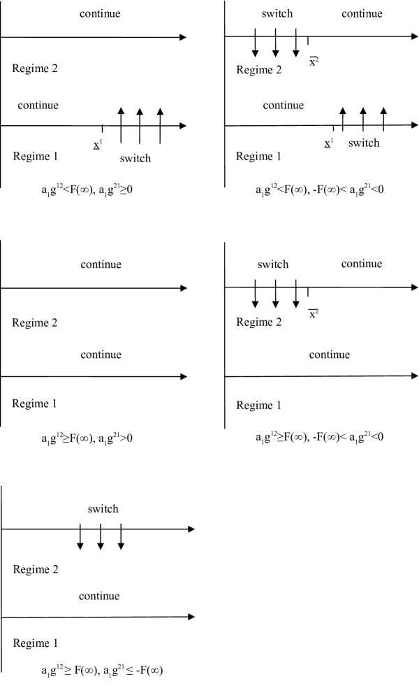
Figure 1: The structure of switching regions

The main result of this section is the following characterization of the switching regions of the optimal switching problem (3.5), which are also demonstrated in Figure 1.

Theorem 3.1

Suppose that Assumptions 3, 4 and 5 hold. Then we have the following five cases for the switching regions $\mathcal{S}^{1}$ and $\mathcal{S}^{2}$:

1. If $a_{1}g^{12}\geq F(\infty)$ and $a_{1}g^{21}\geq 0$, then, $\mathcal{S}^{1}=\phi,\mathcal{S}^{2}=\phi$;

2. If $a_{1}g^{12}\geq F(\infty)$ and $-F(\infty)<a_{1}g^{21}<0$, then, $\mathcal{S}^{1}=\phi,\mathcal{S}^{2}=(0,\overline{x}^{2}]$, where $\overline{x}^{2}\in(0,\infty)$;

3. If $a_{1}g^{12}\geq F(\infty)$ and $a_{1}g^{21}\leq-F(\infty)$, then, $\mathcal{S}^{1}=\phi,\mathcal{S}^{2}=(0,\infty)$;

4. If $a_{1}g^{12}<F(\infty)$ and $a_{1}g^{21}\geq 0$, then, $\mathcal{S}^{1}=[\underline{x}^{1},\infty),\mathcal{S}^{2}=\phi$, where $\underline{x}^{1}\in(0,\infty)$.

5. If $a_{1}g^{12}<F(\infty)$ and $-F(\infty)<a_{1}g^{21}<0$, then, $\mathcal{S}^{1}=[\underline{x}^{1},\infty),\mathcal{S}^{2}=(0,\overline{x}^{2}]$, where $\underline{x}^{1},\overline{x}^{2}\in(0,\infty)$.

3.1 The Structure of Switching Regions: Proof of Theorem 3.1

The proof relies on several basic properties of the value function $v(\cdot)$, and the associated comparison principle. First, we prove that the value function $v(\cdot)$ has at most linear growth and is Lipschitz continuous by employing the optimal switching representation (3.5). The proof is adapted from Ly Vath and Pham [18], and is provided in the Appendix.

Proposition 3.2

Suppose that Assumptions 3 and 4 hold. Then the value function $v(\cdot)$ of the optimal switching problem has at most linear growth,

$$|v^{i}(x)|\leq C(1+x),$$

and is Lipschitz continuous,

$$|v^{i}(x)-v^{i}(\bar{x})|\leq C|x-\bar{x}|,$$

for $i=1,2$ and $x,\bar{x}\in\mathbb{R}^{+}$.

Given the above linear growth property and the Lipschitz continuous property of $v(\cdot)$, the nonlinear Feynman-Kac formula (see Section 6 of [8]) then implies that $v(\cdot)$ is the unique (viscosity) solution to the following system of ODEs:

$$-\mathcal{L}v^{i}(x)+a_{1}v^{i}(x)=\lambda\max\left\{0,v^{j}(x)-g^{ij}-v^{i}(x)\right\}+h^{i}(x)$$ (3.6)

for $i=1,2$ and $j=3-j$, where the operator $\mathcal{L}=\frac{1}{2}\sigma^{2}x^{2}\frac{d^{2}}{dx^{2}}+bx\frac{d}{dx}$. Note that (3.6) are actually penalized equations for the system of variational inequalities:

$$\min\{-\mathcal{L}v^{i}(x)+a_{1}v^{i}(x)-h^{i}(x),v^{i}(x)-v^{j}(x)+g^{ij}\}=0.$$

Moreover, the following comparison principle for (3.6) also holds, whose proof is also provided in the Appendix for completeness.

Proposition 3.3

Suppose that $\underline{v}^{i}(\cdot)$ is the subsolution of the following ODE:

$$-\mathcal{L}\underline{v}^{i}(x)+a_{1}\underline{v}^{i}(x)\leq 0$$ (3.7)

for $x\in\mathbb{R}^{+}$, and that $\underline{v}^{i}(\cdot)$ has at most linear growth. Then $\underline{v}^{i}(x)\leq 0$ for $x\in\mathbb{R}^{+}$. The supersolution property also holds for $\overline{v}^{i}(\cdot)$ in a similar way.

The structure of the switching region $\mathcal{S}^{1}$

Define $G_{1}(x)=v^{1}(x)-v^{2}(x)+g^{12}$. From (3.6), it is easy to see that $G_{1}(\cdot)$ is the solution of the following ODE:

$$-\mathcal{L}G_{1}(x)+a_{1}G_{1}(x)=\lambda(-G_{1}(x))^{+}-\lambda(G_{1}(x)-g^{12}-g^{21})^{+}+a_{1}g^{12}-F(x).$$ (3.8)

From Proposition 3.2, $G_{1}(\cdot)$ has at most linear growth and is Lipschitz continuous. The switching region $\mathcal{S}^{1}=\{x\in(0,\infty):G_{1}(x)\leq 0\}$.

Lemma 3.4

Suppose that Assumptions 3, 4 and 5 hold. If there exists $x^{0}\in\mathcal{S}^{1}$, then $[x^{0},\infty)\in\mathcal{S}^{1}$. Hence, if $\mathcal{S}^{1}\neq\phi$, then $\bar{x}^{1}=\infty$.

Proof. Since $G_{1}(\cdot)$ is Lipschitz continues, its derivative ${G_{1}^{\prime}}(x)=\frac{d}{dx}G_{1}(x)$ is bounded. Moreover. from (3.8), it is easy to see ${G_{1}^{\prime}}(\cdot)$ is the subsolution of the following ODE:

$$-\frac{1}{2}\sigma^{2}x^{2}\frac{d^{2}G_{1}^{\prime}}{dx^{2}}-(b+\sigma^{2})x\frac{dG_{1}^{\prime}}{dx}+(a_{1}-b+\lambda H(-G_{1})+\lambda H(G_{1}-g^{12}-g^{21}))G_{1}^{\prime}=-F^{\prime}(x)\leq 0,$$ (3.9)

where $H(x)=\mathbf{1}_{[0,\infty)}(x)$. Since $a_{1}>b$, by using the subsolution property in Proposition 3.3, we obtain $G_{1}^{\prime}(x)\leq 0$. Thus, if $G_{1}(x^{0})\leq 0$, then $G_{1}(x)\leq 0$ for $x\in[x^{0},\infty)$.   

Proposition 3.5

Suppose that Assumptions 3, 4 and 5 hold. Then

1. If $a_{1}g^{12}\geq F(\infty)$, then $\underline{x}^{1}=\infty$, i.e. $\mathcal{S}^{1}=\phi$.

2. If $a_{1}g^{12}<F(\infty)$, then $\underline{x}^{1}\in(0,\infty)$ and $\mathcal{S}^{1}=[\underline{x}^{1},\infty)$.

Proof.

1. We claim that $\underline{x}^{1}\neq 0$. If not, then $\underline{x}^{1}=\inf\mathcal{S}^{1}=0$, so that $G_{1}(0)\leq 0$ by the continuity of $G_{1}(\cdot)$ on $(0,\infty)$. On the other hand, from (3.8), we have $G_{1}(0)=\dfrac{a_{1}g^{12}}{a_{1}+\lambda}>0$, which is a contradiction.

   Now we show that $\underline{x}^{1}=\infty$. Suppose not. Then $0<\underline{x}^{1}=\inf\mathcal{S}^{1}<\infty$. Due to the continuity of $G_{1}(\cdot)$ on $(0,\infty)$, we have $G_{1}(\underline{x}^{1})=0$, so $\underline{x}^{1}\in\mathcal{S}^{1}$. From Lemma 3.4, $[\underline{x}^{1},\infty)\in\mathcal{S}^{1}$, and $G_{1}(x)\leq 0$ for $x\in[\underline{x}^{1},\infty)$. Therefore, (3.8) reduces to

   $$-\mathcal{L}G_{1}(x)+(a_{1}+\lambda)G_{1}(x)=a_{1}g^{12}-F(x)>0$$

   on $[\underline{x}^{1},\infty)$. But from the supersolution property in Proposition 3.3, we get $G_{1}(x)>0$ for $x\in[\underline{x}^{1},\infty)$, which is obscured.

2. Similar to the proof in 1, we have $\underline{x}^{1}\neq 0$. Therefore, we only need to prove $\underline{x}^{1}\neq\infty$. If not, then $G_{1}(x)>0$ for $x\in(0,\infty)$, and (3.8) reduces to

   $$-\mathcal{L}G_{1}(x)+a_{1}G_{1}(x)=-\lambda(G_{1}(x)-g^{12}-g^{21})^{+}+a_{1}g^{12}-F(x).$$

   By the comparison principle in Proposition 3.3, we have $G_{1}(x)\leq G(x)$, where $G(x)$ is the solution with linear growth to the following ODE:

   $$-\mathcal{L}G(x)+a_{1}G(x)=a_{1}g^{12}-F(x).$$

   The Feynman-Kac formula implies that

   $$G(x)=\mathbf{E}[\int^{\infty}_{0}e^{-a_{1}t}(a_{1}g^{12}-F(X^{x}_{t}))dt]$$

   By Fatou lemma, we have

   $$G(\infty)=\varlimsup_{x\to\infty}\mathbf{E}[\int^{\infty}_{0}e^{-a_{1}t}(rg^{12}-F(X^{x}_{t}))dt]\leq\mathbf{E}[\int^{\infty}_{0}e^{-a_{1}t}(rg^{12}-F(\infty))dt]<0.$$

   Thus, we have $G_{1}(\infty)<0$. This is a contradiction.

 

The financial intuition behind Proposition 3.5 is that the structure of the switching region of the regime $1$ depends on the “instant loss” of the switching cost $g^{12}$ and the “net running profit” $F=h^{2}-h^{1}$. If $a_{1}g^{12}\geq F(\infty)$, which means the loss by switching can not be compensated by the net running profit, then one has no interest to switch; If $a_{1}g^{12}<F(\infty)$, which means the net running profit may exceed the loss due to the switching cost in some state, then one may switch when the net running profit reaches some level at Poisson arrival times.

The Structure of the switching region $\mathcal{S}^{2}$

Define $G_{2}(x)=v^{2}(x)-v^{1}(x)+g^{21}$, which is the solution to the following ODE:

$$-\mathcal{L}G_{2}(x)+a_{1}G_{2}(x)=\lambda(-G_{2}(x))^{+}-\lambda(G_{2}(x)-g^{21}-g^{12})^{+}+a_{1}g^{21}+F(x).$$ (3.10)

From Proposition 3.2, $G_{2}(\cdot)$ has at most linear growth and is Lipschitz continuous. The switching region $\mathcal{S}^{2}=\{x\in(0,\infty):G_{2}(x)\leq 0\}$.

Lemma 3.6

Suppose that Assumptions 3, 4 and 5 hold. If there exists $x^{0}\in\mathcal{S}^{2}$, then $(0,x^{0}]\in\mathcal{S}^{2}$. Hence, if $\mathcal{S}^{2}\neq\phi$, then $\underline{x}^{2}=0$.

Proof. From Lemma 3.4, we have $G_{2}^{\prime}(x)=-G_{1}^{\prime}(x)\geq 0$. Thus, if $G_{2}(x^{0})\leq 0$, then $G_{2}(x)\leq 0$ for $x\in(0,x^{0}]$.   

Proposition 3.7

Suppose that Assumptions 3, 4 and 5 hold. Then

1. If $a_{1}g^{21}\geq 0$, then $\overline{x}^{2}=0$, i.e. $\mathcal{S}^{2}=\phi$.

2. If $-F(\infty)<a_{1}g^{21}<0$, then $\overline{x}^{2}\in(0,\infty)$ and $\mathcal{S}^{2}=(0,\overline{x}_{2}]$.

3. If $a_{1}g^{21}\leq-F(\infty)$, then $\mathcal{S}^{2}=(0,\infty)$.

Proof.

1. If there exists $\overline{x}^{2}\in(0,\infty]$, then $G_{2}(0)<0$ (From (3.10), it is easy to see that there does not exist any interval in which $G_{2}$ keeps constant.). From (3.10), we can see that $G_{2}(0)=\dfrac{a_{1}g^{21}}{a_{1}+\lambda}\geq 0$. This is a contradiction, so $\bar{x}^{2}=\sup\mathcal{S}^{2}$ must be zero.

2. Thanks to Lemma 3.6, we only need to show that $\overline{x}^{2}\neq 0$ and $\overline{x}^{2}\neq\infty$.

   If $\overline{x}_{2}=0$, then $G_{2}(x)>0$ for $x\in(0,\infty)$, and $G_{2}(0)\geq 0$ due to the continuity of $G_{2}(\cdot)$. Hence, (3.10) reduces to

   $$-\mathcal{L}G_{2}(x)+a_{1}G_{2}(x)=-\lambda(G_{2}(x)-g^{21}-g^{12})^{+}+a_{1}g^{21}+F(x).$$

   By the comparison principle in Proposition 3.3, we have $G_{2}(x)\leq G(x)$, where $G(x)$ is the solution with linear growth to the following ODE:

   $$-\mathcal{L}G(x)+a_{1}G(x)=a_{1}g^{21}+F(x).$$

   By continuity of both $G_{2}(\cdot)$ and $G(\cdot)$, $G_{2}(0)\leq G(0)=g_{21}<0$, which is a contradiction. Thus, we have $\overline{x}^{2}\neq 0$.

   If $\overline{x}_{2}=\infty$, i.e. $G_{2}(x)\leq 0$ for $x\in(0,\infty)$, then (3.10) reduces to

   $$-\mathcal{L}G_{2}(x)+(a_{1}+\lambda)G_{2}(x)=a_{1}g^{21}+F(x).$$

   The Feynman-Kac formula implies that

   $$G_{2}(x)=\mathbf{E}[\int^{\infty}_{0}e^{-(a_{1}+\lambda)t}(a_{1}g^{21}+F(X^{x}_{t}))dt]$$

   By Fatou lemma, we have

   $$G_{2}(\infty)=\varliminf_{x\to\infty}\mathbf{E}[\int^{\infty}_{0}e^{-(a_{1}+\lambda)t}(a_{1}g^{21}+F(X^{x}_{t}))dt]\geq\mathbf{E}[\int^{\infty}_{0}e^{-(a_{1}+\lambda)t}(a_{1}g^{21}+F(\infty))dt]>0$$

   This is a contradiction. Thus, we have $\overline{x}^{2}\neq\infty$.

3. Suppose that $G_{0}(\cdot)$ is the solution with linear growth to the following ODE:

   $$-\mathcal{L}G_{0}(x)+(a_{1}+\lambda)G_{0}(x)=a_{1}g^{21}+F(x).$$

   Since $a_{1}g^{21}+F(x)<a_{1}g^{21}+F(\infty)\leq 0$, the subsolution property in Proposition 3.3 implies that $G_{0}(x)\leq 0$ for $x\in(0,\infty)$. Thus $G_{0}(\cdot)$ is one solution with linear growth to (3.10). Due to the uniqueness of the solution to (3.10), we must have $G_{2}(x)=G_{0}(x)\leq 0$ for $x\in(0,\infty)$, which means $\mathcal{S}^{2}=(0,\infty)$.

 

The financial intuition behind Proposition 3.7 is that (1) when the switching cost from a “higher regime” to a “lower regime” is non-negative, it is unnecessary to switch; (2) if the switching cost is negative and can “compensate” the loss due to switching to a “lower regime” in some state, the player would switch to a “lower regime” at some level at Poisson arrival times; (3) if the profit from switching cost exceeds the maximum loss from the “net running profit”, the player would switch to a “lower regime” from a “higher regime” at Poisson arrival times.

Appendix A Appendix

A.1 Proof of Proposition 2.1

Existence of solutions to the infinite horizon BSDE system (2.3)

The idea is to truncate the infinite horizon BSDE system (2.3) on $[0,\infty)$ to a finite horizon one on $[0,n]$ for any $n\geq 0$:

$$Y_{t}^{i}(n)=\int_{t}^{n}f_{s}^{i}(Y_{s}(n),Z_{s}(n))+\lambda\max\left\{0,\mathcal{M}Y_{s}^{i}(n)-Y_{s}^{i}(n)\right\}ds-\int_{t}^{n}Z_{s}^{i}(n)dW_{s}.$$ (A.1)

Then for $n\geq m\geq 0$, we consider the difference of two truncated equations truncated on different time intervals $[0,n]$ and $[0,m]$:

$$Y_{t}^{i}(n)-Y_{t}^{i}(m)= \ \int_{t}^{n}f_{s}^{i}(Y_{s}(n),Z_{s}(n))-f_{s}^{i}(Y_{s}(m),Z_{s}(m))+f_{s}^{i}(Y_{s}(m),Z_{s}(m))\mathbf{1}_{\{s\geq m\}}ds$$

$$+\int_{t}^{n}\lambda\left(\mathcal{M}Y_{s}^{i}(n)-Y_{s}^{i}(n)\right)^{+}-\lambda\left(\mathcal{M}Y_{s}^{i}(m)-Y_{s}^{i}(m)\right)^{+}+\lambda\left(\mathcal{M}Y_{s}^{i}(m)-Y_{s}^{i}(m)\right)^{+}\mathbf{1}_{\{s\geq m\}}ds$$

$$-\int_{t}^{n}\left(Z_{s}^{i}(n)-Z_{s}^{i}(m)+Z_{s}^{i}(m)\mathbf{1}_{\{s\geq m\}}\right)dW_{s}$$

Note that $Y_{t}(m)=Z_{t}(m)=0$ on $\{t\geq m\}$. Hence, we have

$$f_{s}^{i}(Y_{s}(m),Z_{s}(m))\mathbf{1}_{\{s\geq m\}}=f_{s}^{i}(0,0)\mathbf{1}_{\{s\geq m\}},$$

and

$$\lambda\left(\mathcal{M}Y_{s}^{i}(m)-Y_{s}^{i}(m)\right)^{+}\mathbf{1}_{\{s\geq m\}}=Z_{s}^{i}(m)\mathbf{1}_{\{s\geq m\}}=0.\\$$

Now apply Itô’s formula to $e^{2at}|Y_{t}(n)-Y_{t}(m)|^{2}$,

$$\ e^{2at}|Y_{t}({n})-Y_{t}({m})|^{2}$$

$$= \ -\int_{t}^{n}2ae^{2as}|Y_{s}(n)-Y_{s}(m)|^{2}ds$$

$$\ +\int_{t}^{n}2e^{2as}(Y_{s}(n)-Y_{s}(m))^{*}\left(f_{s}(Y_{s}(n),Z_{s}(n))-f_{s}(Y_{s}(m),Z_{s}(m))+f_{s}(0,0)\mathbf{1}_{\{s\geq m\}}\right)ds$$

$$\ +\int_{t}^{n}2\lambda e^{2as}[Y_{s}(n)-Y_{s}(m)]^{*}\left((\mathcal{M}Y_{s}(n)-Y_{s}(n))^{+}-(\mathcal{M}Y_{s}(m)-Y_{s}(m))^{+}\right)ds$$

$$\ -\int_{t}^{n}2e^{2as}(Y_{s}(n)-Y_{s}(m))^{*}(Z_{s}(n)-Z_{s}(m))dW_{s}$$

$$\ -\int_{t}^{n}e^{2as}||Z_{s}(n)-Z_{s}(m)||^{2}ds.$$ (A.2)

By the monotone condition and Lipschitz condition in Assumption 1, the second term on the RHS of (A.1) is dominated by

$$\int_{t}^{n}-2a_{1}e^{2as}|Y_{s}(n)-Y_{s}(m)|^{2}+2a_{2}e^{2as}|Y_{s}(n)-Y_{s}(m)|\times||Z_{s}(n)-Z_{s}(m)||ds$$

$$+\int_{m}^{n}2e^{2as}(Y_{s}(n)-Y_{s}(m))^{*}f_{s}(0,0)ds$$

$$\leq \int_{t}^{n}-2a_{1}e^{2as}|Y_{s}(n)-Y_{s}(m)|^{2}ds$$

$$+\int_{t}^{n}\delta_{1}^{2}a_{2}^{2}e^{2as}|Y_{s}(n)-Y_{s}(m)|^{2}+\frac{1}{\delta_{1}^{2}}e^{2as}||Z_{s}(n)-Z_{s}(m)||^{2}ds$$

$$+\int_{m}^{n}\delta_{2}^{2}a_{2}^{2}e^{2as}|Y_{s}(n)-Y_{s}(m)|^{2}+\frac{1}{\delta_{2}^{2}a_{2}^{2}}e^{2as}|f_{s}(0,0)|^{2}ds$$ (A.3)

for any constants $\delta_{1},\delta_{2}$, where we used the elementary inequality $2ab\leq\frac{1}{\delta^{2}}a^{2}+\delta^{2}b^{2}$.

Similarly, the third term on the RHS of (A.1) is dominated by

$$\int_{t}^{n}2\lambda e^{2as}|Y_{s}(n)-Y_{s}(m)|\times|(\mathcal{M}Y_{s}(n)-Y_{s}(n))-(\mathcal{M}Y_{s}(m)-Y_{s}(m))|ds$$

$$\leq \int_{t}^{n}2\lambda e^{2as}\left(|Y_{s}(n)-Y_{s}(m)|^{2}+|Y_{s}(n)-Y_{s}(m)|\times|\mathcal{M}Y_{s}(n)-\mathcal{M}Y_{s}(m)|\right)ds$$

$$\leq \int_{t}^{n}2\lambda e^{2as}\left(1+\frac{1}{2}+\frac{d}{2}\right)|Y_{s}(n)-Y_{s}(m)|^{2}ds$$ (A.4)

By plugging (A.1) and (A.1) into (A.1), and choosing $\delta_{1}^{2}>1$ and $\delta_{1}^{2}+\delta_{2}^{2}<\delta$, and $a$ as in the structure condition (2.6), we obtain

$$e^{2at}|Y_{t}({n})-Y_{t}({m})|^{2}+(1-\frac{1}{\delta_{1}^{2}})\int_{t}^{n}e^{2as}||Z_{s}(n)-Z_{s}(m)||^{2}ds$$

$$\leq \int_{m}^{n}\frac{1}{\delta_{2}^{2}a_{2}^{2}}e^{2as}|f_{s}(0,0)|^{2}ds-\int_{t}^{n}2e^{2as}(Y_{s}(n)-Y_{s}(m))^{*}(Z_{s}(n)-Z_{s}(m))dW_{s}$$

Taking expectation at $t=0$, we have

$$\mathbf{E}\left[\int_{0}^{n}e^{2as}||Z_{s}(n)-Z_{s}(m)||^{2}ds\right]\leq\frac{\delta_{1}^{2}}{(\delta_{1}^{2}-1)\delta_{2}^{2}a_{2}^{2}}\mathbf{E}\left[\int_{m}^{n}e^{2as}|f_{s}(0,0)|^{2}ds\right]\downarrow 0$$

as $m,n\uparrow\infty$. Hence, $(Z(n))_{n\geq 0}$ is a Cauchy sequence in $\mathcal{H}^{2}_{a}(\mathbb{R}^{d\times n})$, and converges to some limit process, denoted as $Z$. On the other hand, taking supremum over $t\geq 0$, and then taking expectation, we obtain

$$\mathbf{E}\left[\sup_{t\geq 0}e^{2at}|Y_{t}({n})-Y_{t}({m})|^{2}\right]$$

$$\leq \frac{1}{\delta_{2}^{2}a_{2}^{2}}\mathbf{E}\left[\int_{m}^{n}e^{2as}|f_{s}(0,0)|^{2}ds\right]+\mathbf{E}\left[\sup_{t\geq 0}|\int_{t}^{\infty}2e^{2as}(Y_{s}(n)-Y_{s}(m))^{*}(Z_{s}(n)-Z_{s}(m))dW_{s}|\right]$$

The standard argument by using the BDG inequality implies that the martingale term is in fact uniformly integrable, so by taking $m,n\uparrow\infty$, we deduce that $(Y(n))_{n\geq 0}$ is a Cauchy sequence in $\mathcal{S}^{2}_{a}(\mathbb{R}^{d})$, and converges to some limit process, denoted as $Y$. It is standard to check that $(Y,Z)$ indeed satisfies (2.3), so in order to verify that they are one solution to the infinite horizon BSDE system (2.3), we only need to prove that

$$\lim_{t\uparrow\infty}\mathbf{E}\left[e^{2at}|Y_{t}|^{2}\right]=0.$$ (A.5)

Indeed, since $(Y(n))_{n\geq 0}$ is a Cauchy sequence in $\mathcal{S}^{2}_{a}(\mathbb{R}^{d})$, for any $\epsilon>0$, there exists $n$ large enough such that

$$\mathbf{E}\left[e^{2at}|Y_{t}|^{2}\right]\leq 2\mathbf{E}\left[e^{2at}|Y_{t}-Y_{t}(n)|^{2}\right]+2\mathbf{E}\left[e^{2at}|Y_{t}(n)|^{2}\right]<2\epsilon+2\mathbf{E}\left[e^{2at}|Y_{t}(n)|^{2}\right].$$

Letting $t\uparrow\infty$ and noting $Y_{t}(n)=0$ for $t\geq n$, we obtain the desired convergence (A.5).

Uniqueness of solutions to the infinite horizon BSDE system (2.3)

The proof of uniqueness is similar to the proof of the existence, so we only sketch it. Let $(Y,Z)$ and $(\tilde{Y},\tilde{Z})$ be two solutions to the infinite horizon BSDE system (2.3). Denote $\delta Y_{t}^{i}=Y_{t}^{i}-\tilde{Y}_{t}^{i}$, and $\delta Z_{t}^{i}=Z_{t}^{i}-\tilde{Z}_{t}^{i}$. Then $(\delta Y,\delta Z)$ satisfies the following equation:

$$\delta Y^{i}_{t}=\delta Y_{T}^{i}+\int_{t}^{T}F_{s}^{i}(Y_{s},Z_{s})-F_{s}^{i}(\tilde{Y}_{s},\tilde{Z}_{s})ds-\int_{t}^{T}\delta Z^{i}_{s}dW_{s},$$

where we denote

$$F_{s}^{i}(y,z)=f^{i}_{s}(y,z)+\lambda\max\{0,\mathcal{M}y^{i}-y^{i}\}$$

for any $(y,z)\in\mathbb{R}^{d}\times\mathbb{R}^{d\times n}$.

Apply Itô’s formula to $e^{2at}|\delta Y_{t}|^{2}$,

$$e^{2at}|\delta Y_{t}|^{2}= \ e^{2aT}|\delta Y_{T}|^{2}-\int_{t}^{T}2ae^{2as}|\delta Y_{s}|^{2}ds$$

$$\ +\int_{t}^{T}2e^{2as}(\delta Y_{s})^{*}\left(F_{s}(Y_{s},Z_{s})-F_{s}(\tilde{Y}_{s},\tilde{Z}_{s})\right)ds$$

$$\ -\int_{t}^{T}2e^{2as}(\delta Y_{s})^{*}\delta Z_{s}dW_{s}-\int_{t}^{T}e^{2as}||\delta Z_{s}||^{2}ds.$$ (A.6)

Using the monotone condition and the Lipschitz condition in Assumption 1, we get

$$e^{2at}|\delta Y_{t}|^{2}+(1-\frac{1}{\delta_{1}^{2}})\int_{t}^{T}e^{2as}||\delta Z_{s}||^{2}ds$$

$$\leq \ e^{2aT}|\delta Y_{T}|^{2}-\left(2a+2a_{1}-\delta_{1}^{2}a_{2}^{2}-(d+3)\lambda\right)\int_{t}^{T}e^{2as}|\delta Y_{s}|^{2}ds-\int_{t}^{T}2e^{2as}(\delta Y_{s})^{*}\delta Z_{s}dW_{s}.$$ (A.7)

Choosing $\delta_{1}^{2}=\delta$ and taking expectation on (A.1) at $t=0$, we obtain

$$(1-\frac{1}{\delta})\mathbf{E}\left[\int_{0}^{T}e^{2as}||\delta Z_{s}||^{2}ds\right]\leq\mathbf{E}\left[e^{2aT}|\delta Y_{T}|^{2}\right].$$

Since $\lim_{T\uparrow\infty}\mathbf{E}\left[e^{2aT}|\delta Y_{T}|^{2}\right]=0$, we conclude that

$$\mathbf{E}\left[\int_{0}^{\infty}e^{2as}||\delta Z_{s}||^{2}ds\right]=0.$$

On the other hand, choosing $\delta_{1}^{2}=\delta$, taking supremum over $t\geq 0$, and take expectation on (A.1), we get

$$\mathbf{E}\left[\sup_{t\geq 0}e^{2at}|\delta Y_{t}|^{2}\right]\leq\mathbf{E}\left[e^{2aT}|\delta Y_{T}|^{2}\right]+\mathbf{E}\left[\sup_{t\geq 0}|\int_{t}^{T}2e^{2as}(\delta Y_{s})^{*}\delta Z_{s}dW_{s}|\right].$$

Since $\lim_{T\uparrow\infty}\mathbf{E}\left[e^{2aT}|\delta Y_{T}|^{2}\right]=0$, and the martingale is uniformly integrable, we conclude that

$$\mathbf{E}\left[\sup_{t\geq 0}e^{2at}|\delta Y_{t}|^{2}\right]=0.$$

A.2 Proof of Proposition 3.2

For any switching strategy $u\in\mathcal{K}_{i}(0,\lambda)$, the running profit of (3.5) is dominated by

$$\mathbf{E}\left[\int_{0}^{\infty}e^{-a_{1}s}h^{u_{s}}(X_{s}^{x})\right]\leq C\mathbf{E}\left[\int_{0}^{\infty}e^{-a_{1}s}X_{s}^{x}ds\right]=\frac{Cx}{a_{1}-b},$$ (A.8)

where we used $h(0)=0$ and the Lipschitz continuity of $h(\cdot)$. The switching cost of (3.5) is dominated by

$$-\sum_{k=1}^{M}e^{-a_{1}T_{k}}g^{\alpha_{k-1},\alpha_{k}}\leq\max_{j=1,2}[-g^{ij}]$$ (A.9)

for any $M\geq 1$, which can be proved by induction as in [18]. Indeed, (A.9) obviously holds for $M=1$. Suppose (A.9) holds for $M\geq 1$, we consider $M+1$. When $g^{\alpha_{M},\alpha_{M+1}}\geq 0$, (A.9) obviously holds as $a_{1}\geq 0$. When $g^{\alpha_{M},\alpha_{M+1}}\leq 0$, we have

$$-\sum_{k=1}^{M+1}e^{-a_{1}T_{k}}g^{\alpha_{k-1},\alpha_{k}} =-\sum_{k=1}^{M-1}e^{-a_{1}T_{k}}g^{\alpha_{k-1},\alpha_{k}}-(e^{-a_{1}T_{M}}g^{\alpha_{M-1},\alpha_{M}}+e^{-a_{1}T_{M+1}}g^{\alpha_{M},\alpha_{M+1}})$$

$$\leq-\sum_{k=1}^{M-1}e^{-a_{1}T_{k}}g^{\alpha_{k-1},\alpha_{k}}-e^{-a_{1}T_{M}}(g^{\alpha_{M-1},\alpha_{M}}+g^{\alpha_{M},\alpha_{M+1}})$$

$$\leq-\sum_{k=1}^{M-1}e^{-a_{1}T_{k}}g^{\alpha_{k-1},\alpha_{k}}-e^{-a_{1}T_{M}}g^{\alpha_{M-1},\alpha_{M+1}}\leq\max_{j=1,2}[-g^{ij}].$$

Combining (A.8) and (A.9) gives us

$$\mathbf{E}\left[\int_{0}^{\infty}e^{-a_{1}s}h^{u_{s}}(X_{s}^{x})ds-\sum_{k\geq 1}e^{-a_{1}T_{k}}g^{\alpha_{k-1},\alpha_{k}}\right]\leq\frac{Cx}{a_{1}-b}+\max_{j=1,2}[-g^{ij}].$$

From the arbitrariness of $u\in\mathcal{K}_{i}(0,\lambda)$, we obtain that the RHS of the above inequality is the upper bound of $v^{i}(\cdot)$.

On the other hand, for $j=1,2$, choose a switching strategy as

$$u_{s}=i\mathbf{1}_{[0,T_{1}]}(s)+j\mathbf{1}_{[T_{1},\infty)}(s).$$

Then, since $h\geq 0$,

$$\mathbf{E}\left[\int_{0}^{\infty}e^{-a_{1}s}h^{u_{s}}(X_{s}^{x})ds-\sum_{k\geq 1}e^{-a_{1}T_{k}}g^{\alpha_{k-1},\alpha_{k}}\right]\geq\mathbf{E}\left[-e^{a_{1}T_{1}}g^{ij}\right]=\frac{-\lambda}{a_{1}+\lambda}g^{ij}\geq\frac{\lambda}{a_{1}+\lambda}\max_{j=1,2}\{-g^{ij}\}.$$

Once again, from the arbitrariness of $u\in\mathcal{K}_{i}(0,\lambda)$, we obtain that the RHS of the above inequality is the lower bound of $v^{i}(\cdot)$, so $v^{i}(\cdot)$ has at most linear growth.

We conclude by showing the Lipschitz continuity of $v^{i}(\cdot)$. Indeed, for $x,\bar{x}\in\mathbb{R}^{+}$,

$$|v^{i}(x)-v^{i}(\bar{x})| \leq\sup_{u\in\mathcal{K}_{i}(0,\lambda)}\mathbf{E}\left[\int_{0}^{\infty}e^{-a_{1}s}|h^{u_{s}}(X_{s}^{x})-h^{u_{s}}(X_{s}^{\bar{x}})|ds\right]$$

$$\leq\sup_{u\in\mathcal{K}_{i}(0,\lambda)}\mathbf{E}\left[\int_{0}^{\infty}e^{-a_{1}s}C|X_{s}^{x}-X_{s}^{\bar{x}}|ds\right]$$

$$=\mathbf{E}\left[\int_{0}^{\infty}e^{-a_{1}s}C|x-\bar{x}|e^{(b-\frac{1}{2}\sigma^{2})s+\sigma W_{s}}ds\right]$$

$$=\frac{C}{a_{1}-b}|x-\bar{x}|.$$

A.3 Proof of Proposition 3.3

We only prove the subsolution property, as the supersolution property is similar. The proof relies on the comparison principle for the ODE (3.7) on a finite interval. For any $x^{0}\in(0,\infty)$ and $\epsilon>0$, since $b<a_{1}$, we can choose $p>0,q>1$ such that

$$\frac{1}{2}\sigma^{2}p(p+1)-bp-a_{1}\leq 0.$$

$$\frac{1}{2}\sigma^{2}q(q-1)+bq-a_{1}\leq 0.$$

With such $p,q$, we then choose $C_{1},C_{2},C_{3}>0$ such that

$$C_{1}(x^{0})^{q}+\frac{C_{2}}{(x^{0})^{p}}+C_{3}\leq\epsilon.$$

Now we consider the following auxiliary function

$$\underline{w}^{i}(x)=\underline{v}^{i}(x)-\left(C_{1}x^{q}+\frac{C_{2}}{x^{p}}+C_{3}\right).$$

Then we have

$$(-\mathcal{L}+a_{1})\underline{w}^{i}(x)=(-\mathcal{L}+a_{1})\underline{v}^{i}(x)+C_{1}x^{q}\left(\frac{1}{2}\sigma^{2}q(q-1)+bq-a_{1}\right)+\frac{C_{2}}{x^{p}}\left(\frac{1}{2}\sigma^{2}p(p+1)-bp-a_{1}\right)-a_{1}C_{3}.$$

Since $\underline{v}^{i}(\cdot)$ is the subsolution to the ODE (3.7) and the terms involving $p,q$ are negative by the choice of $p,q$, we obtain that $(-\mathcal{L}+a_{1})\underline{w}^{i}(x)\leq 0$ for $x\in(0,\infty)$.

On the other hand, by the linear growth condition of $\underline{v}^{i}(\cdot)$, there exits $\underline{x}$ and $\overline{x}$ such that $x^{0}\in[\underline{x},\overline{x}]$ and $\underline{w}^{i}(\overline{x})\leq 0$ and $\underline{w}^{i}(\underline{x})\leq 0$. Then the comparison principle for the ODE (3.7) on a finite interval $[\underline{x},\overline{x}]$ implies that $\underline{w}^{i}(x^{0})\leq 0$, and therefore, $\underline{v}^{i}(x^{0})\leq\epsilon$. Letting $\epsilon\downarrow 0$, we obtain $\underline{v}^{i}(x^{0})\leq 0$ for any $x^{0}\in(0,\infty)$.

References

• [1] Bayraktar, E. and Egami, M., On the one-dimensional optimal switching problem, Mathematics of Operations Research, 35(1), (2010), 140–159.
• [2] Bayraktar, E. and Ludkovski, M., A Sequential Tracking of a Hidden Markov Chain Using Point Process Observations, Stochastic Processes and Their Applications, 119(6), (2009), 1792–1822.
• [3] Bensoussan, A. and Lions, J. L., Impulse control and quasivariational inequalities, Gauthier-Villars, Paris, (1984).
• [4] Brekke, K. and Oksendal, B., Optimal switching in an economic activity under uncertainty. SIAM J. Control Optim., 32(4), (1994), 1021-1036.
• [5] Briand, P., and Ying H., Stability of BSDEs with random terminal time and homogenization of semilinear elliptic PDEs, Journal of Functional Analysis, 155(2), (1998), 455-494.
• [6] Carmona, R. and Ludkovski, M., Pricing asset scheduling flexibility using optimal switching, Applied Mathematical Finance, 15, (2008), 405–447.
• [7] Dai, M., Zhang, Q., and Zhu, Q., Trend following trading under a regime switching model, SIAM Journal on Financial Mathematics, 1, (2010), 780–810.
• [8] Darling, R. W. R., and Pardoux, E., Backwards SDE with random terminal time and applications to semilinear elliptic PDE, The Annals of Probability, 25(3), (1997), 1135-1159.
• [9] Duckworth, K. and Zervos, M., A model for investment decisions with switching costs. The Annals of Applied probability, (2001), 239-260.
• [10] Dupuis, P. and Wang, H., Optimal stopping with random intervention times, Adv. in Appl. Probab., 34(1), (2002), 141-157.
• [11] El Karoui, N., Peng, S. and Quenez, M. C., Backward stochastic differential equations in finance, Mathematical Finance, 7(1), (1997), 1–71.
• [12] Hamadène, S. and Jeanblanc, M., On the starting and stopping problem: Application in reversible investments, Math. Oper. Res., 32 (1), (2007), 182–192.
• [13] Hamadène, S. and Zhang, J., Switching problem and related system of reflected backward SDEs, Stochastic Processes and Their Applications, 120, (2010), 403–426.
• [14] Hu, Y. and Tang, S., Multi-dimensional BSDE with oblique reflection and optimal switching, Probab. Theory Related Fields, 147, (2010), 89–121.
• [15] Lempa, J., Optimal stopping with information constraint. Applied Mathematics and Optimization, 66(2), (2012), 147-173.
• [16] Liang, G., Stochastic control representations for penalized backward stochastic differential equations, Working paper, (2013).
• [17] Liang, G., Lütkebohmert, E. and Wei, W., Funding liquidity, debt tenor structure, and creditor’s belief: An exogenous dynamic debt run model, Working paper, (2013).
• [18] Ly Vath, V., and Pham, H., Explicit solution to an optimal switching problem in the two-regime case, SIAM Journal on Control and Optimization, 46(2), (2007), 395–426.
• [19] Ma, J. and Yong, J., Forward-backward stochastic differential equations and their applications, Lecture Notes in Mathematics, Springer-Verlag, Berlin, (1999).
• [20] Pardoux, É. and Peng, S. G., Adapted solution of a backward stochastic differential equation, Systems & Control Letters, 14(1), (1990), 55–61.
• [21] Pham, H., Continuous-time stochastic control and optimization with financial applications, Springer-Verlag, Berlin, (2009).
• [22] Pham, H., Ly Vath, V., and Zhou, X. Y., Optimal switching over multiple regimes, SIAM Journal on Control and Optimization, 48(4), (2009), 2217–2253.
• [23] Porchet, A., Touzi, N. and Warin, X., Valuation of power plants by utility indifference and numerical computation, Math. Methods Oper. Res., 70(1), (2009), 47–75.
• [24] Tang, S. and Yong, J., Finite horizon stochastic optimal switching and impulse controls with a viscosity solution approach. Stochastics: An International Journal of Probability and Stochastic Processes, 45(3-4), (1993), 145-176.
• [25] Yong, J. and Zhou, X. Y., Stochastic controls: Hamiltonian systems and HJB equations, Springer-Verlag, New York, (1999).
Refer to caption