Stochastic Bound Majorization

Abstract

Recently a majorization method for optimizing partition functions of log-linear models was proposed alongside a novel quadratic variational upper-bound. In the batch setting, it outperformed state-of-the-art first- and second-order optimization methods on various learning tasks. We propose a stochastic version of this bound majorization method as well as a low-rank modification for high-dimensional data-sets. The resulting stochastic second-order method outperforms stochastic gradient descent (across variations and various tunings) both in terms of the number of iterations and computation time till convergence while finding a better quality parameter setting. The proposed method bridges first- and second-order stochastic optimization methods by maintaining a computational complexity that is linear in the data dimension and while exploiting second order information about the pseudo-global curvature of the objective function (as opposed to the local curvature in the Hessian).

1 Introduction

Stochastic learning algorithms are of central interest in machine learning due to their simplicity and, as opposed to batch methods, their low memory and computational complexity requirements [1, 2, 3]. For instance, stochastic learning algorithms are commonly used to train deep belief networks (DBNs) [4, 5] which perform extremely well on tasks involving massive data-sets [6, 7]. Stochastic algorithms are also broadly used to train Conditional Random Fields (CRFs) [8], solve maximum likelihood problems [9] and perform variational inference [10].

Most stochastic optimization approaches fall into two groups: first-order methods and second-order methods. Popular first-order methods include stochastic gradient descent (SGD) [11] and its many extensions [12, 13, 14, 15, 16, 17]. These methods typically have low computational cost per iteration (such as $\mathcal{O}(d)$ where $d$ is the data dimensionality) and either sub-linear (most stochastic gradient methods) or linear (as shown recently in [12]) convergence rate which makes them particularly relevant for large-scale learning. Despite its simplicity, SGD has many drawbacks: it has slow asymptotic convergence to the optimum [8], it has limited ability to handle certain regularized learning problems such as $l_{1}$-regularization [18], it requires step-size tuning and it is difficult to parallelize [19]. Many works have tried to incorporate second-order information (i.e. Hessian) into the optimization problem to improve the performance of traditional SGD methods. A straightforward way of doing so is to simply replace the gain in SGD with the inverse of the Hessian matrix which, when naively implemented, induces a computational complexity of $\mathcal{O}(d^{3})$. This makes the approach impractical for large problems. The trade-offs in large-scale learning for various prototypical batch and stochastic learning algorithms are conveniently summarized in [20]). Therein, several new methods are developed, including variants of Newton’s method which use both gradient and Hessian information to compute the descent direction. By carefully exploring different first- and second-order techniques, the overall computational complexity of optimization can be reduced as in the Stochastic Meta-Descent (SMD) algorithm [21]. Although it still uses the gradient direction to converge, SMD also efficiently exploits certain Hessian-vector products to adapt the gradient step-size. The algorithm is shown to converge to the same quality solution as limited-memory BFGS (LBFGS) an order of magnitude faster for CRF training [8]. There also exists stochastic versions of quasi-Newton methods like online BFGS and online LBFGS [22], the latter applicable to large-scale problems, which while using convenient size mini-batches performs comparably to a well-tuned natural gradient descent [23] on the task of training CRFs, but at the same time is more scalable. In each iteration the inverse of the Hessian, that is assumed to have no negative eigenvalues, is estimated. Computational complexity of this online LBFGS method is $\mathcal{O}(md)$ per iteration, where $m$ is the size of the buffer used to estimate the inverse of the curvature. The method degrades (large $m$) for sparse data-sets. Another second-order stochastic optimization approach proposed in the literature explores diagonal approximations of the Hessian matrix or Gauss-Newton matrix[5, 24]. In some cases this approach appears to be overly simplistic [25], but turned out successful in very particular applications, i.e. for learning with linear Support Vector Machines [24]. There is also a large body of work on stochastic second-order methods particularly successful in training deep belief network like Hessian-free optimization [25]. Finally, there are also many hybrid methods using existing stochastic optimization tools as building blocks and merging them to obtain faster and more robust learning algorithms [9, 26].

This paper contributes to the family of existing second-order stochastic optimization methods with a new algorithm that is using a globally guaranteed quadratic bound with a curvature different than the Hessian. Therefore our approach is not merely a variant of Newton’s method. This is a stochastic version of a recently proposed majorization method [27] which performed maximum (latent) conditional likelihood problems more efficiently than other state-of-the-art first- and second- order batch optimization methods like BFGS, LBFGS, steepest descent (SD), conjugate gradient (CG) and Newton. The corresponding stochastic bound majorization method is compared with a well-tuned SGD with either constant or adaptive gain in $l_{2}$-regularized logistic regression and turns out to outperform competitor methods in terms of the number of iterations, the convergence time and even the quality of the obtained solution measured by the test error and test likelihood.

2 Preliminaries

A staggering number of machine learning and statistics frameworks involve linear combinations or cascaded linear combinations of soft-maximum functions:

$$s(\bm{\theta})=\sum_{j=1}^{t}\gamma_{i}\log\sum_{y}h(y)\exp(\bm{\theta}^{\top}{\bf f}(y)),$$

where $\bm{\theta}\in\mathbb{R}^{d}$ is a parameter vector, ${\bf f}:\Omega\rightarrow\mathbb{R}^{d}$ is any vector-valued function mapping an input $y$ to some arbitrary vector (we assume $\Omega$ is finite and $|\Omega|=n$ is enumerable), $t$ is the size of the data-set and $\gamma_{i}$ is some non-negative weight. These functions emerge in multi-class logistic regression, CRFs [28], hidden variable problems, DBNs [29], discriminatively trained speech recognizers [30] and maximum entropy problems [31]. For simplicity, we focus herein on the CRF training problem in particular. CRFs use the density model:

$$p(y|x_{j},\bm{\theta})=\frac{1}{Z_{x_{j}}(\bm{\theta})}h_{x_{j}}(y)\exp(\bm{\theta}^{\top}{\bf f}_{x_{j}}(y)),$$

where $\{(x_{1},y_{1}),\dots,(x_{t},y_{t})\}$ are iid input-output pairs and $Z_{x_{j}}(\bm{\theta})$ is a partition function: $Z_{x_{j}}(\bm{\theta})=\sum_{y\in\Omega_{j}}h_{x_{j}}(y)\exp(\bm{\theta}^{\top}{\bf f}_{x_{j}}(y))$. Following the maximum likelihood approach, the objective function to maximize in this setting is:

$$J(\bm{\theta})=\sum_{j=1}^{t}\left[\log\frac{h_{x_{j}}(y_{j})}{Z_{x_{j}}(\bm{\theta})}+\bm{\theta}^{\top}{\bf f}_{x_{j}}(y_{j})\right]-\frac{\lambda}{2}\|\bm{\theta}\|^{2},$$ (1)

where $\lambda$ is a regularization hyper-parameter. Let $J(\bm{\theta})=\sum_{j=1}^{t}J_{j}(\bm{\theta})$, where $J_{j}(\bm{\theta})=\log\frac{h_{x_{j}}(y_{j})}{Z_{x_{j}}(\bm{\theta})}+\bm{\theta}^{\top}{\bf f}_{x_{j}}(y_{j})-\frac{\lambda}{2t}\|\bm{\theta}\|^{2}$. For large numbers of data points $t$, and potentially large dimensionality $d$, summations in Equation 1 need not be handled in a batch form, but rather, can be processed stochastically or semi-stochastically. We next review the most commonly used stochastic algorithm, SGD, which will be a key comparator for our stochastic bound majorization algorithm.

2.1 Stochastic gradient descent methods

Batch gradient descent updates the parameter vector $\bm{\theta}$ after seeing the entire training data-set using the following formula:

$$\bm{\theta}=\bm{\theta}-\eta{\bm{\mu}}(\bm{\theta})=\bm{\theta}-\eta\sum_{j=1}^{t}{\bm{\mu}}_{j}(\bm{\theta}),$$

where ${\bm{\mu}}(\bm{\theta})=\bigtriangledown_{\bm{\theta}}J(\bm{\theta})$, ${\bm{\mu}}_{j}(\bm{\theta})=\bigtriangledown J_{j}(\bm{\theta})$ and $\eta$ is typically chosen via line search. In contrast, stochastic gradient descent updates the parameter vector $\bm{\theta}$ after seeing each training data point (resp. each mini-batch of data points) as follows:

$$\bm{\theta}_{i+1}=\bm{\theta}_{i}-\eta_{i}{\bm{\mu}}_{j}(\bm{\theta}_{i}),\>\>\>\>\>\>\>\>\text{resp.}\>\>\bm{\theta}_{i+1}=\bm{\theta}_{i}-\eta_{i}\sum_{j=1}^{m}{\bm{\mu}}_{j}(\bm{\theta}_{i}),$$

where $\bm{\theta}_{i}$ is the current parameter vector, $\eta_{i}$ is the current gain or step-size, and $m<<t$ is the size of the mini-batch. We assume a data point is randomly selected and take its index to be $j$. We intentionally index $\bm{\theta}$ with $i$ and $i+1$ to emphasize that the update is done after seeing single example (resp. mini-batch of examples). For the batch method, we do not index $\bm{\theta}$ since the update is done after passing through the entire data-set (epoch). In the experimental section we explore two existing variants of stochastic gradient descent: one with constant gain (SGD) and one with adaptive gain (ASGD). For the latter, we consider two strategies for modifying the gain and present the results for the better one (in Section 5 the absence of a $\tau$ value indicates that the second strategy is better since it does not require a $\tau$ parameter):

• $\eta_{i}=\frac{\tau}{\tau+i}\eta_{0}$

• $\eta_{i}=\frac{\eta_{0}}{i}$,                       where $\eta_{0},\tau>0$   are tuning parameters.

2.2 Batch bound majorization algorithm

Input Parameters $\tilde{\bm{\theta}},{\bf f}(y),h(y)\>\forall y\in\Omega$ Init $z\rightarrow 0^{+},{\bf g}={\bm{0}},{\bm{\Sigma}}=z{\bf I}\>\>$ For each $y\in\Omega$ { $\>\>\>\>\>\>\>\>\>\>\>\>\alpha=h(y)\exp(\tilde{\bm{\theta}}^{\top}{\bf f}(y));\>\>{\bf l}={\bf f}(y)-{\bf g}$ $\>\>\>\>\>\>\>\>\>\>\>\>\beta=\frac{\tanh(\frac{1}{2}\log(\alpha/z))}{2\log(\alpha/z)};\>\>\kappa=\frac{\alpha}{z+\alpha}$ $\>\>\>\>\>\>\>\>\>\>\>\>{\bm{\Sigma}}\>\>\>\!\!\!\;\!\;+\!=\beta{\bf l}{\bf l}^{\top}$ $\>\>\>\>\>\>\>\>\>\>\>\>{\bf g}\>\>\!\!\>\;\>+\!=\kappa{\bf l}$ $\>\>\>\>\>\>\>\>\>\>\>\>z\>\;\>\>+\!=\alpha\>\>\>\>\>\>\>\}$ Output $z,{\bf g},{\bm{\Sigma}}$

Algorithm 1 Batch Bound

Theorem 1

Algorithm 1 finds $z,{\bf g},{\bm{\Sigma}}$ such that $z\exp(\frac{1}{2}(\bm{\theta}-\tilde{\bm{\theta}})^{\top}{\bm{\Sigma}}(\bm{\theta}-\tilde{\bm{\theta}})+(\bm{\theta}-\tilde{\bm{\theta}})^{\top}\!{\bf g})$ upper-bounds $Z(\bm{\theta})=\sum_{y}h(y)\exp(\bm{\theta}^{\top}{\bf f}(y))$ for any $\bm{\theta},\tilde{\bm{\theta}},{\bf f}(y)\in\mathbb{R}^{d}$ and $h(y)\in\mathbb{R}^{+}$ for all $y\in\Omega$.

The stochastic bound majorization algorithm proposed in this paper is a stochastic variant of the batch method described in [27]. The bound is depicted in Theorem 1. The figure near Algorithm 1 shows typical bounds the algorithm recovers (in blue) and also shows (in green) examples what happens when the bound’s ${\bm{\Sigma}}$ matrix is replaced by the Hessian matrix which yields a second-order approximation to the function. These tight quadratic bounds facilitate majorization: solving an optimization problem by iteratively finding the optima of simple bounds on it [32] as popularized by the Expectation-Maximization (EM) algorithm [33]. Majorization was shown to achieve faster and monotonically convergent performance in CRF learning and maximum latent conditional likelihood problems with a clear advantage over state-of-the-art first- and second-order batch methods [27]. The batch bound majorization algorithm applied to Equation 1 updates the parameter vector $\bm{\theta}$ after seeing the entire training data-set using the following formula:

$$\bm{\theta}=\bm{\theta}-\eta{\bm{\Sigma}}^{-1}(\bm{\theta})\mu(\bm{\theta}),$$ (2)

where ${\bm{\Sigma}}(\bm{\theta})=\sum_{j=1}^{t}{\bm{\Sigma}}_{j}(\bm{\theta})+\lambda{\bf I}$, ${\bm{\mu}}(\bm{\theta})=\sum_{j=1}^{t}{\bm{\mu}}_{j}(\bm{\theta})=\sum_{j=1}^{t}({\bf g}_{j}(\bm{\theta})-{\bf f}_{j}(y_{j}))+\lambda\bm{\theta}$. Here, each ${\bm{\Sigma}}_{j}$ and ${\bf g}_{j}$ is computed using Algorithm 1 (for details see [27]) and $\eta\in(0,2)$ guarantees monotonic improvement [34] (typically we set $\eta=1$).

3 Stochastic bound majorization algorithm

The intuition behind stochastic gradient descent is to compute the gradient over a single representative data-point rather than an iterative computation (namely a summation) over all data-points. This allows us to interleave parameter updates into the gradient computation rather than wait for it to terminate after a full epoch. We herewith extend this intuition into a bound majorization setting. Unfortunately, the update rule for majorization involves a matrix inverse rather than a simple sum across the data. We will re-cast this update rule as an iterative computation over the data-set which will then admit a stochastic incarnation.

3.1 Full-rank version

Notice that the batch update in Equation 2 is the solution of the linear system:

$$\left(\sum_{j=1}^{t}{\bm{\Sigma}}_{j}+\lambda{\bf I}\right){\bm{\delta}}=\sum_{j=1}^{t}{\bm{\mu}}_{j}$$

For the ease of notation we denote ${\bm{\Sigma}}_{j}(\bm{\theta})$ as ${\bm{\Sigma}}_{j}$ and ${\bm{\mu}}_{j}(\bm{\theta})$ as ${\bm{\mu}}_{j}$. Rewrite the linear system as ${\bm{\Sigma}}{\bm{\delta}}={\bf u}$. We then define the inverse matrix ${\bf M}={\bm{\Sigma}}^{-1}$ and write the solution as ${\bm{\delta}}={\bf M}{\bf u}$. Clearly, the matrix inversion cannot be performed each time we process a single data-point in a stochastic setting since a computational complexity of $\mathcal{O}(d^{3})$ is prohibitive in a stochastic setting. Therefore, consider an online version of Algorithm 1 which computes the matrix inversion of ${\bm{\Sigma}}$ incrementally using the Sherman-Morrison formula $({\bm{\Sigma}}+{\bf q}_{i}{\bf q}_{i}^{\top})^{-1}={\bm{\Sigma}}^{-1}-({\bm{\Sigma}}^{-1}{\bf q}_{i}{\bf q}_{i}^{\top}{\bm{\Sigma}}^{-1})/(1+{\bf q}_{i}^{\top}{\bm{\Sigma}}^{-1}{\bf q}_{i})$. Sherman-Morrison works with the inverse matrix ${\bf M}={\bm{\Sigma}}^{-1}$ instead. Initialize ${\bf M}_{0}=\frac{1}{\lambda}{\bf I}$ and incrementally increase ${\bf M}$ using the update rule:

$${\bf M}_{i+1}={\bf M}_{i}-\frac{{\bf M}_{i}{\bf q}_{i}{\bf q}_{i}^{\top}{\bf M}_{i}}{1+{\bf q}_{i}^{\top}{\bf M}_{i}{\bf q}_{i}},\>\>\>\>\>\text{where}\>\>\>{\bf q}_{i}=\sqrt{\beta_{i}}({\bf f}_{i}-{\bf g}_{i})=\sqrt{\beta_{i}}{\bf l}_{i},$$

where the index $i$ ranges over all rank $1$ updates to the matrix ${\bm{\Sigma}}$ for all elements of $\Omega$ as well as $j=1,\dots,t$. Finally, the solution is obtained by multiplying ${\bf M}$ with ${\bf u}$. This avoids $\mathcal{O}(d^{3})$ inversion and solves the linear system in $\mathcal{O}(tnd^{2})$. Let $T=tn$. We will now reformulate the batch update from Equation 2 by using the Sherman-Morrison technique. For the ease of notation, introduce $\bm{\xi}$’s such that $\forall_{i=1,2,\dots,T}{\bm{\mu}}_{i}={\bm{\mu}}_{i-1}+\bm{\xi}_{i-1}$ (thus $\bm{\xi}_{i-1}=\kappa_{i-1}{\bm{l}}_{i-1}-{\bm{f}}_{i-1}+\lambda\bm{\theta}/t$).

$$\bm{\theta}=\bm{\theta}-\eta{\bm{M}_{T}}{\bm{\mu}}_{T}=\bm{\theta}-\eta\left[{\bm{M}}_{T-1}-\frac{{\bm{M}}_{T-1}{\bf q}_{T-1}{\bf q}_{T-1}^{\top}{\bm{M}}_{T-1}}{1+{\bf q}_{T-1}^{\top}{\bf M}_{T-1}{\bf q}_{T-1}}\right]({\bm{\mu}}_{T-1}+\bm{\xi}_{T-1})$$

$$=\bm{\theta}-\eta{\bm{M}}_{T-1}{\bm{\mu}}_{T-1}-\eta{\bm{M}}_{T-1}\bm{\xi}_{T-1}+\frac{{\bm{M}}_{T-1}{\bf q}_{T-1}{\bf q}_{T-1}^{\top}{\bm{M}}_{T-1}}{1+{\bf q}_{T-1}^{\top}{\bf M}_{T-1}{\bf q}_{T-1}}{\bm{\mu}}_{T-1}$$

$$+\frac{{\bm{M}}_{T-1}{\bf q}_{T-1}{\bf q}_{T-1}^{\top}{\bm{M}}_{T-1}}{1+{\bf q}_{T-1}^{\top}{\bf M}_{T-1}{\bf q}_{T-1}}\bm{\xi}_{T-1}.$$

We can further expand ${\bm{M}}_{T-1}{\bm{\mu}}_{T-1}$ as:

$${\bm{M}}_{T-1}{\bm{\mu}}_{T-1}=\left[{\bm{M}}_{T-2}-\frac{{\bm{M}}_{T-2}{\bf q}_{T-2}{\bf q}_{T-2}^{\top}{\bm{M}}_{T-2}}{1+{\bf q}_{T-2}^{\top}{\bf M}_{T-2}{\bf q}_{T-2}}\right]({\bm{\mu}}_{T-2}+\bm{\xi}_{T-2})$$

$$={\bm{M}}_{T-2}{\bm{\mu}}_{T-2}+{\bm{M}}_{T-2}\bm{\xi}_{T-2}-\frac{{\bm{M}}_{T-2}{\bf q}_{T-2}{\bf q}_{T-2}^{\top}{\bm{M}}_{T-2}}{1+{\bf q}_{T-2}^{\top}{\bf M}_{T-2}{\bf q}_{T-2}}{\bm{\mu}}_{T-2}-\frac{{\bm{M}}_{T-2}{\bf q}_{T-2}{\bf q}_{T-2}^{\top}{\bm{M}}_{T-2}}{1+{\bf q}_{T-2}^{\top}{\bf M}_{T-2}{\bf q}_{T-2}}\bm{\xi}_{T-2}$$

and again we can further expand ${\bm{M}}_{T-2}{\bm{\mu}}_{T-2}$ as:

$${\bm{M}}_{T-2}{\bm{\mu}}_{T-2}=\left[{\bm{M}}_{T-3}-\frac{{\bm{M}}_{T-3}{\bf q}_{T-3}{\bf q}_{T-3}^{\top}{\bm{M}}_{T-3}}{1+{\bf q}_{T-3}^{\top}{\bf M}_{T-3}{\bf q}_{T-3}}\right]({\bm{\mu}}_{T-3}+\bm{\xi}_{T-3})$$

$$={\bm{M}}_{T-3}{\bm{\mu}}_{T-3}+{\bm{M}}_{T-3}\bm{\xi}_{T-3}-\frac{{\bm{M}}_{T-3}{\bf q}_{T-3}{\bf q}_{T-3}^{\top}{\bm{M}}_{T-3}}{1+{\bf q}_{T-3}^{\top}{\bf M}_{T-3}{\bf q}_{T-3}}{\bm{\mu}}_{T-3}-\frac{{\bm{M}}_{T-3}{\bf q}_{T-3}{\bf q}_{T-3}^{\top}{\bm{M}}_{T-3}}{1+{\bf q}_{T-3}^{\top}{\bf M}_{T-3}{\bf q}_{T-3}}\bm{\xi}_{T-3}.$$

We repeat these steps. In the last step we expand ${\bm{M}}_{1}{\bm{\mu}}_{1}$. We can combine these results and write the following update rule:

$$\bm{\theta}=\bm{\theta}-\eta{\bm{M}}_{T}{\bm{\mu}}_{T}=\bm{\theta}-\eta{\bm{M}}_{0}{\bm{\mu}}_{0}-\eta\sum_{c=0}^{T-1}\left[{\bm{M}}_{c}\bm{\xi}_{c}-\frac{{\bm{M}}_{c}{\bf q}_{c}{\bf q}_{c}^{\top}{\bm{M}}_{c}}{1+{\bf q}_{c}^{\top}{\bf M}_{c}{\bf q}_{c}}{\bm{\mu}}_{c}-\frac{{\bm{M}}_{c}{\bf q}_{c}{\bf q}_{c}^{\top}{\bm{M}}_{c}}{1+{\bf q}_{c}^{\top}{\bf M}_{c}{\bf q}_{c}}\bm{\xi}_{c}\right]$$

$$=\bm{\theta}-\eta\sum_{c=0}^{T-1}\left[\left({\bm{M}}_{c}-\frac{{\bm{M}}_{c}{\bf q}_{c}{\bf q}_{c}^{\top}{\bm{M}}_{c}}{1+{\bf q}_{c}^{\top}{\bf M}_{c}{\bf q}_{c}}\right)\bm{\xi}_{c}-\frac{{\bm{M}}_{c}{\bf q}_{c}{\bf q}_{c}^{\top}{\bm{M}}_{c}}{1+{\bf q}_{c}^{\top}{\bf M}_{c}{\bf q}_{c}}{\bm{\mu}}_{c}\right]$$

The last inequality comes from the fact that ${\bm{\mu}}_{0}$ is initialized as ${\bm{\mu}}_{0}={\bm{0}}$. We have thus rewritten the batch majorization update rule for the parameters as an iterative summation over the data. Analogous to the conversion of a batch gradient descent algorithm into SGD, the most natural way to convert the batch bound majorization algorithm to its stochastic version is to interleave updates of the parameter $\bm{\theta}$ rather than waiting for the full summation to terminate (after an epoch) before allowing $\bm{\theta}$ to update. This permits us to now write a fully stochastic update rule on the parameter vector $\bm{\theta}$ (in original notation):

$$\begin{split}\bm{\theta}_{i+1}=\bm{\theta}_{i}-\eta_{i}\left[\left({\bm{M}}_{j}(\bm{\theta}_{i})-\frac{{\bm{M}}_{j}(\bm{\theta}_{i}){\bf q}_{j}(\bm{\theta}_{i}){\bf q}_{j}(\bm{\theta}_{i})^{\top}{\bm{M}}_{j}(\bm{\theta}_{i})}{1+{\bf q}_{j}(\bm{\theta}_{i})^{\top}{\bf M}_{j}(\bm{\theta}_{i}){\bf q}_{j}(\bm{\theta}_{i})}\right)\bm{\xi}_{j}(\bm{\theta}_{i})\right.\\ \left.-\frac{{\bm{M}}_{j}(\bm{\theta}_{i}){\bf q}_{j}(\bm{\theta}_{i}){\bf q}_{j}(\bm{\theta}_{i})^{\top}{\bm{M}}_{j}(\bm{\theta}_{i})}{1+{\bf q}_{j}(\bm{\theta}_{i})^{\top}{\bf M}_{j}(\bm{\theta}_{i}){\bf q}_{j}(\bm{\theta}_{i})}{\bm{\mu}}_{j}(\bm{\theta}_{i})\right]\end{split}$$

Input: $\lambda\in\mathbb{R}^{+}$, $\eta$ Initialize: ${\bm{\theta}}\in\mathbb{R}^{d}$, $\bm{\phi}=zeros(d)$, ${\bm{M}}=\frac{1}{\lambda}{\bm{I}}$, ${\bm{\mu}}={\bm{0}}$ while not converged { select data point $j$ $z\rightarrow 0^{+};\>\>{\bm{g}}={\bm{0}}$ For each $y\in\Omega$   { $\>\>\>\>\>\>\>\>\>\>\>\>\>\alpha=h_{j}(y)\exp({\bm{\theta}}^{\top}{{\bm{f}}_{j}}(y));\>\>{\bm{l}}={{\bm{f}}}_{j}(y)-{\bm{g}};\>\>\beta=\frac{\tanh(\frac{1}{2}\log(\alpha/z)}{2\log(\alpha/z)};\>\>\kappa=\frac{\alpha}{z+\alpha}\>\>\>\>\>\>\>\>\>\>\>\>\>\>\>\>\>\>\>\>\>\>\>\>\>\>\>\>\>\>$ $\>\>\>\>\>\>\>\>\>\>\>\>\>\bm{\xi}=\kappa{\bm{l}}-{\bm{f}}_{j}+\lambda\bm{\theta}/t$ $\>\>\>\>\>\>\>\>\>\>\>\>\>{\bm{N}}\>\>\>\;=\frac{{\bm{M}}\beta{\bm{l}}{\bm{l}}^{\top}{\bm{M}}}{1+\beta{\bm{l}}^{\top}{\bm{M}}{\bm{l}}}$ $\>\>\>\>\>\>\>\>\>\>\>\>\>{\bm{M}}\>\!\!\;-\!={\bm{N}}$ $\>\>\>\>\>\>\>\>\>\>\>\>\>\bm{\phi}\>\>\;+\!={\bm{M}}\bm{\xi}-{\bm{N}}{\bm{\mu}}$ $\>\>\>\>\>\>\>\>\>\>\>\>\>{\bm{g}}\>\>\>\!\>\!\;+\!=\kappa{\bm{l}}$ $\>\>\>\>\>\>\>\>\>\>\>\>\>{\bm{\mu}}\>\>\;+\!=\bm{\xi}$ $\>\>\>\>\>\>\>\>\>\>\>\>\>z\>\;\>\>+\!=\alpha$   } $\bm{\theta}\>\;-\!=\eta\bm{\phi}$   }

Algorithm 2 Stochastic Bound

The stochastic bound majorization algorithm also readily admits mini-batches. Algorithm 2 captures the full-rank version of the proposed algorithm (we always use constant step size $\eta=\frac{1}{t}$).

We have also investigated many other potential variants of Algorithm 2 including heuristics borrowed from other stochastic algorithms in the literature [12]. Some heuristics involved using memory to store previous values of updates, gradients and second order matrix information. Remarkably, all such heuristics and modifications slowed down the convergence of Algorithm 2.

On caveat remains. The computational complexity of the proposed stochastic bound majorization method is $\mathcal{O}(nd^{2})$ per iteration which is less appealing than the $\mathcal{O}(nd)$ complexity of SGD. This shortcoming is resolved in the next subsection.

3.2 Low-rank version

We next provide a low-rank version of Algorithm 2 to maintain a $\mathcal{O}(nd)$ run-time per stochastic update. Consider the update on $\bm{\phi}$ inside the loop over $y$ in Algorithm 2. This update can be rewritten as

$$\bm{\phi}+\!={\bm{M}}\bm{\xi}-{\bm{N}}{\bm{\mu}}={\bm{M}}\bm{\xi}-({\bm{M}}_{old}-{\bm{M}}){\bm{\mu}}=({\bm{\Sigma}})^{-1}\bm{\xi}-(({\bm{\Sigma}}_{old})^{-1}-({\bm{\Sigma}})^{-1}){\bm{\mu}},$$

where ${\bf M}_{old}$ and ${\bm{\Sigma}}_{old}$ are the matrices that, after being updated, become ${\bf M}$ and ${\bm{\Sigma}}$ respectively: ${\bf M}={\bf M}_{old}-{\bf N}_{old}$, ${\bf M}_{old}={\bm{\Sigma}}_{old}^{-1}$ and ${\bm{\Sigma}}={\bm{\Sigma}}_{old}+{\bf q}_{old}{\bf q}_{old}^{\top}={\bm{\Sigma}}_{old}+{\beta}_{old}{\bf l}_{old}{\bf l}_{old}^{\top}$ (rank $1$ update). We can store the matrix ${\bm{\Sigma}}$ using a low-rank representation ${\bf V}^{\top}{\bf S}{\bf V}+{\bf D}$, where $k$ is a rank ($k<<d$), ${\bf V}\in\mathbb{R}^{k\times d}$ is orthonormal, ${\bf S}\in\mathbb{R}^{k\times k}$ is positive semi-definite and ${\bf D}\in\mathbb{R}^{d\times d}$ is non-negative diagonal. We can directly update ${\bf V}$, ${\bf S}$ and ${\bf D}$ online rather than incrementing matrix ${\bm{\Sigma}}$ by a rank $1$ update. In the case of batch bound majorization method this still guarantees an overall upper bound [27]. We directly apply this technique as well in our stochastic setting. Due to space constraints we will not present this technique (we refer the reader to [27]). Given a low-rank version of the matrix, we use the Woodbury formula to invert it in each iteration: ${\bf\Sigma}^{-1}={\bf D}^{-1}+{\bf D}^{-1}{\bf V}^{\top}({\bf S}^{-1}+{\bf V}{\bf D}^{-1}{\bf V}^{\top})^{-1}{\bf V}{\bf D}^{-1}$. That leads to a low-rank version of Algorithm 2, which requires only $\mathcal{O}(knd)$ work per iteration which is pseudo-linear in dimension if $k$ is assumed to be a logarithmic or constant function of $d$.

4 A motivating example

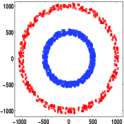
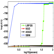
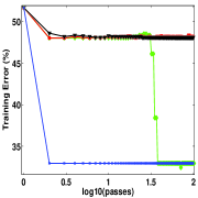
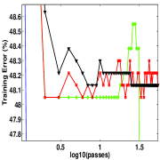
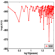
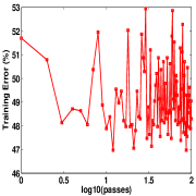
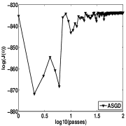
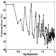
Figure 1: A comparison of LBFGS, SGD, ASGD and SBM for $l_{2}$-regularized logistic regression. From left to right, first row: the data-set, training log-likelihood and error (original and zoomed) vs. passes through the data for LBFGS, SGD ($\eta_{0}=10^{-8}$, $m=1$), ASGD ($\eta_{0}=10^{-5}$, $\tau=1$, $m=1$) and SBM ($\eta_{0}=\frac{1}{t}$, $m=1$), second row: SGD training log-likelihood and error ($\eta_{0}=10^{-7}$) and ASGD training log-likelihood and error ($\eta_{0}=10^{-4}$, $\tau=1$) vs. passes through the data. $\lambda=10^{1}$.

Consider Figure 1 which is an example of a binary classification problem which exposes some of difficulties with SGD. Intuitively, in this example, the gradients in the SGD update rule will point in almost random directions which could lead to very slow progress. Four training algorithms will be compared: SGD, ASGD, stochastic bound majorization algorithm (SBM) and LBFGS. We have tried several parameter settings for SGD and ASGD. The range of tested step size $\eta_{0}$ was as broad as $[10^{-12},1]$. The SGD method however exhibits high instability until the step size is reduced to an unreasonably small value such as $10^{-8}$ (for comparison we also show SGD performance for $\eta_{0}=10^{-7}$). The reason for is that this is a highly symmetric and non-linearly separable data-set. Therefore, the information captured in the gradients is extremely noisy which causes SGD to oscillate and fail to converge in practice. For ASGD we obtained the best and stable result for $\eta_{0}=10^{-5}$ (for comparison we also show ASGD performance for $\eta_{0}=10^{-4}$) and $\tau=1$ (larger values of $\tau$ weaken performance). For both methods we tested the mini-batch size $m$ from $1$ (a single data point) to $10$ and noticed no meaningful difference. Clearly both SGD and ASGD are stuck in solutions that are only slightly better than random guessing. Meanwhile SBM (with $m=1$ and a constant step size $\eta_{0}=\frac{1}{t}$) finds the same solution as a batch LBFGS method. It does so with a single pass through the data and simultaneously outperforming the competitor methods. We emphasize that all methods used as comparators to our algorithm were well-tuned, i.e. the initial gain $\eta_{0}$ is set as high as possible for each method while maintaining stability.

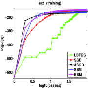
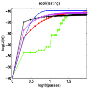
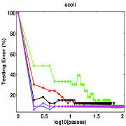
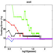
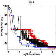
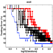
Figure 2: A comparison of LBFGS, SGD, ASGD, SBM and BBM for $l_{2}$-regularized logistic regression. From left to right, first row: training and testing log-likelihood and testing error (original and zoomed) vs. passes through the data for LBFGS, SGD ($\eta_{0}=10^{-2}$, $m=10$), ASGD ($\eta_{0}=10^{-1}$, $\tau=500$, $m=10$), SBM ($\eta_{0}=\frac{1}{t}$, $m=1$) and BBM on the ecoli data-set, second row: testing error (original and zoomed) vs. iterations for LBFGS, SGD and ASGD on the same experiment.

Next, we focus on the ecoli UCI data-set (http://archive.ics.uci.edu/ml/), a simple small-scale classification problem. We compare LBFGS, batch bound majorization method (BBM), SGD, ASGD and SBM. Results are summarized in Figure 2. BBM, which was already shown to outperform leading batch methods [27], performs comparably to ASGD and SGD. The only method that beats BBM is SBM. In the first row of Figure 2, we plot the objective with respect to the number of passes through the data. However, looking more closely at the objective with respect to each iteration (where a single iteration corresponds to a single update of the parameter vector), we note an interesting property of SBM: it clearly remains monotonic in its convergence despite its stochastic nature. This is in contrast to SGD and ASGD which (as expected) fluctuate much more noisily.

Note that, in all experiments in this section and the next, $90\%$ of the data is used for training and the rest for testing, the results are averaged over $10$ random initializations close to the origin and the regularization value $\lambda$ is chosen through crossvalidation. All methods were implemented in C++ using the mex environment under Matlab.

5 Experiments

We next evaluate the performance of the new algorithm empirically. We compare SGD, ASGD and SBM for $l_{2}$-regularized logistic regression on the Mnist^⋆, gisette^∗, SecStr^†, digitl^† and Text^† data-sets. We show two variants of the SBM algorithm: full-rank (on SecSTR and Mnist) and low-rank (on the remaining data-sets). For the experiments with full-rank SBM, we plot the testing log-likelihood and error versus passes through the data (epoch iterations). For the experiments with low-rank SBM, we plot the likelihood versus cpu time. For SGD and ASGD we tested mini-batches of size from $m=1$ to $m=10$ and chose the best setting. For the Mnist data-set we explored mini-batches of up to $m=100$ to achieve optimal SGD behavior. For SBM we always simply used $m=1$. For each data-set, Figure 3 reports the optimal step size $\eta_{0}$ for SGD and ASGD and the optimal parameter $\tau$ for ASGD (if it was necessary). For the full-rank version of SBM we always use $\eta_{0}=\frac{1}{t}$, however for its low-rank version (where we simply assumed $k=1$) we tuned $\eta_{0}$. The chosen value of $\eta_{0}$ is also reported in Figure 3. Clearly, SBM is less prone to over-fitting and achieves higher testing likelihood than SGD and ASGD as well as lower testing error. Simultaneously, SBM exhibits the fastest convergence in terms of the number of passes through the data till convergence. Furthermore, low-rank SBM had the fastest convergence in terms of cpu time, outperforming the leading stochastic first-order methods (SGD and ASGD) as shown in the plots of likelihood over time.

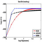
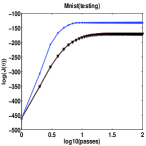
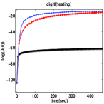
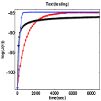
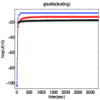
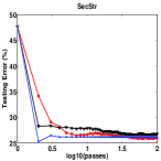
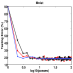
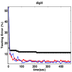
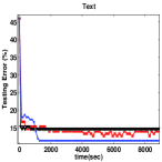
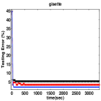
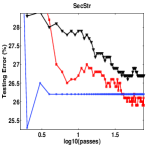
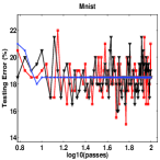
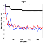
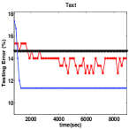
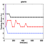
Figure 3: A comparison of SGD, ASGD and SBM for $l_{2}$-regularized logistic regression. From top to bottom: testing log-likelihood and testing error (original and zoomed) vs. passes through the data for data-sets: SecStr ($t=83679$, $n=2$, $d=632$, $\lambda=10^{1}$, SGD ($\eta_{0}=10^{-4}$, $m=10$), ASGD ($\eta_{0}=10^{-1}$, $m=10$) SBM ($\eta_{0}=\frac{1}{t}$, $m=1$, full-rank)), Mnist ($t=10000$, $n=10$, $d=510$, $\lambda=10^{-2}$, SGD ($\eta_{0}=10^{-1}$, $m=100$), ASGD ($\eta_{0}=10^{-1}$, $\tau=10^{5}$, $m=100$) SBM ($\eta_{0}=\frac{1}{t}$, $m=1$, full-rank)), digitl ($t=1500$, $n=2$, $d=1448$, $\lambda=10^{1}$, SGD ($\eta_{0}=10^{-4}$, $m=10$), ASGD ($\eta_{0}=10^{-3}$, $\tau=10^{2}$, $m=10$) SBM ($\eta_{0}=50\cdot\frac{1}{t}$, $m=1$, $k=1$)), Text ($t=1500$, $n=2$, $d=23922$, $\lambda=10^{1}$, SGD ($\eta_{0}=10^{-4}$, $m=10$), ASGD ($\eta_{0}=10^{-2}$, $\tau=10^{3}$, $m=10$) SBM ($\eta_{0}=\frac{1}{t}$, $m=1$, $k=1$)) and gisette ($t=1500$, $n=2$, $d=10002$, $\lambda=10^{0}$, SGD ($\eta_{0}=10^{-3}$, $m=10$), ASGD ($\eta_{0}=10^{-1}$, $\tau=10^{1}$, $m=10$) SBM ($\eta_{0}=100\cdot\frac{1}{t}$, $m=1$, $k=1$)).

6 Conclusion

We have proposed a new stochastic bound majorization method for optimizing the partition function of log-linear models that uses second-order curvature through a global bound (rather than a local Hessian). The method is obtained by applying Sherman-Morrison to the batch update rule to convert it into an iterative summation over the data which can easily be made stochastic by interleaving parameter updates. This (full-rank) stochastic method requires no parameter tuning. A low-rank version of this stochastic update rule makes this effectively second-order method remain linear in the dimensionality of the data. We showed experimentally that the method has significant advantage over the state-of-the-art first-order stochastic methods like SGD and ASGD making majorization competitive in both stochastic and batch settings [27]. Stochastic bound majorization achieves convergence in fewer iterations, in less computation time (when using the low-rank version), and with better final solutions. Future work will involve providing theoretical guarantees for the method as well as application to deep architectures with cascaded linear combinations of soft-max functions.

References

- [1] L. Bottou. Online algorithms and stochastic approximations. In David Saad, editor, Online Learning and Neural Networks. Cambridge University Press, Cambridge, UK, 1998.
- [2] N. Littlestone. Learning quickly when irrelevant attributes abound: A new linear-threshold algorithm. Mach. Learn., 2(4):285–318, April 1988.
- [3] F. Rosenblatt. The perceptron: A probabilistic model for information storage and organization in the brain. Psychological Review, 65(6):386–408, 1958.
- [4] L. Bottou. Stochastic gradient learning in neural networks. In Proceedings of Neuro-Nˆımes. 1991.
- [5] Y. Le Cun, L. Bottou, G. B. Orr, and K.-R. Müller. Efficient backprop. In Neural Networks, Tricks of the Trade, Lecture Notes in Computer Science LNCS 1524. Springer Verlag, 1998.
- [6] A. Krizhevsky, I. Sutskever, and G. E. Hinton. Imagenet classification with deep convolutional neural networks. In NIPS, 2012.
- [7] B. Kingsbury, T. N. Sainath, and H. Soltau. Scalable minimum Bayes risk training of deep neural network acoustic models using distributed Hessian-free optimization. In INTERSPEECH, 2012.
- [8] S. V. N. Vishwanathan, N. N. Schraudolph, M. W. Schmidt, and K. P. Murphy. Accelerated training of conditional random fields with stochastic gradient methods. In ICML, 2006.
- [9] N. Le Roux and A. W. Fitzgibbon. A fast natural Newton method. In ICML, 2010.
- [10] C. Wang and D. M. Blei. Truncation-free online variational inference for Bayesian nonparametric models. In NIPS, 2012.
- [11] H. Robbins and S. Monro. A stochastic approximation method. Annals of Mathematical Statistics, 22:400–407, 1951.
- [12] N. Le Roux, M. W. Schmidt, and F. Bach. A stochastic gradient method with an exponential convergence rate for finite training sets. In NIPS, 2012.
- [13] B. T. Polyak and A. B. Juditsky. Acceleration of stochastic approximation by averaging. SIAM J. Control Optim., 30(4):838–855, July 1992.
- [14] P. Tseng. An incremental gradient(-projection) method with momentum term and adaptive stepsize rule. SIAM J. on Optimization, 8(2):506–531, February 1998.
- [15] Y. Nesterov. Primal-dual subgradient methods for convex problems. Math. Program., 120(1):221–259, 2009.
- [16] H. Kesten. Accelerated stochastic approximation. Annals of Mathematical Statistics, 29(1):41–59, 1958.
- [17] D. Blatt, A. O. Hero, and H. Gauchman. A convergent incremental gradient method with a constant step size. SIAM Journal on Optimization, 18(1):29–51, 2007.
- [18] L. Xiao. Dual averaging methods for regularized stochastic learning and online optimization. In NIPS, 2009.
- [19] Q. V. Le, J. Ngiam, A. Coates, A. Lahiri, B. Prochnow, and A. Y. Ng. On optimization methods for deep learning. In ICML, 2011.
- [20] L. Bottou and O. Bousquet. The tradeoffs of large scale learning. In NIPS, 2007.
- [21] N. N. Schraudolph. Local gain adaptation in stochastic gradient descent. In ICANN, 1999.
- [22] N. N. Schraudolph, J. Yu, and S. Günter. A stochastic quasi-Newton method for online convex optimization. In AISTATS, 2007.
- [23] S.-I. Amari, H. Park, and K. Fukumizu. Adaptive method of realizing natural gradient learning for multilayer perceptrons. Neural Comput., 12(6):1399–1409, June 2000.
- [24] A. Bordes, L. Bottou, and P. Gallinari. Sgd-qn: Careful quasi-Newton stochastic gradient descent. J. Mach. Learn. Res., 10:1737–1754, December 2009.
- [25] J. Martens. Deep learning via Hessian-free optimization. In ICML, 2010.
- [26] M. P. Friedlander and M. W. Schmidt. Hybrid deterministic-stochastic methods for data fitting. SIAM J. Scientific Computing, 34(3), 2012.
- [27] T. Jebara and A. Choromanska. Majorization for CRFs and latent likelihoods. In NIPS, 2012.
- [28] J. D. Lafferty, A. McCallum, and F. C. N. Pereira. Conditional random fields: Probabilistic models for segmenting and labeling sequence data. In ICML, 2001.
- [29] G. E. Hinton, S. Osindero, and Y. W. Teh. A fast learning algorithm for deep belief nets. Neural Computation, 18(7):1527–1554, 2006.
- [30] L.R. Bahl, M. Padmanabhan, D. Nahamoo, and P. S. Gopalakrishnan. Discriminative training of Gaussian mixture models for large vocabulary speech recognition systems. In ICASSP, 1996.
- [31] A. Berger. The improved iterative scaling algorithm: A gentle introduction. Technical report, Carnegie Mellon University, 1997.
- [32] J. De Leeuw and W. J. Heiser. Convergence of correction matrix algorithms for multidimensional scaling. chapter Geometric representations of relational data, Mathesis Press, pages 735–752, 1977.
- [33] A. P. Dempster, N. M. Laird, and D. B. Rubin. Maximum likelihood from incomplete data via the EM algorithm. Journal of the Royal Statistical Society, Series B, 39(1):1–38, 1977.
- [34] R. Salakhutdinov and S. T. Roweis. Adaptive overrelaxed bound optimization methods. In ICML, 2003.