Lifshitz-sector mediated SUSY breaking

Abstract

We propose a novel mechanism of SUSY breaking by coupling a Lorentz-invariant supersymmetric matter sector to non-supersymmetric gravitational interactions with Lifshitz scaling. The improved UV properties of Lifshitz propagators moderate the otherwise uncontrollable ultraviolet divergences induced by gravitational loops. This ensures that both the amount of induced Lorentz violation and SUSY breaking in the matter sector are controlled by $\Lambda_{\textrm{HL}}^{2}/M_{P}^{2}$, the ratio of the Hořava-Lifshitz cross-over scale $\Lambda_{\textrm{HL}}$ to the Planck scale $M_{P}$. This ratio can be kept very small, providing a novel way of explicitly breaking supersymmetry without reintroducing fine-tuning. We illustrate our idea by considering a model of scalar gravity with Hořava-Lifshitz scaling coupled to a supersymmetric Wess-Zumino matter sector, in which we compute the two-loop SUSY breaking corrections to the masses of the light scalars due to the gravitational interactions and the heavy fields.

1 Introduction

Supersymmetry (SUSY) is a vastly studied framework, motivated by its ability to solve the gauge hierarchy problem. The latter belongs to the class of “technical naturalness” problems, and is usually formulated in terms of the quadratic divergences plaguing the Higgs mass term in the effective potential. In the absence of protection mechanisms, based for example on symmetries, the physical mass of the Higgs field is naturally driven towards the cutoff of the theory unless some extreme fine-tuning of parameters is invoked. Since the quadratic divergences are scheme dependent –absent, for example, in dimensional regularization– and hence unphysical, one may want to re-state the same problem in an alternative way: the Higgs mass is sensitive to generic New Physics in the form of heavy states, which may couple to the Higgs field either directly or via other gauge and matter fields of the Standard Model (SM). For example, generic heavy states of mass $M$ would normally give rise to finite threshold contributions to the Higgs mass of the form $\frac{M^{2}}{16\pi^{2}}$, which again tend to drive the physical mass towards unacceptably large values so that an ad hoc fine adjustment of the Higgs mass is required.

Supersymmetry solves this problem by automatically forcing the cancellation of threshold contributions between fermionic and bosonic degrees of freedom in the ultraviolet (UV). However, since SUSY is not realized exactly in Nature, there must be new fields and interactions responsible for its breaking. If the main phenomenological motivation for SUSY is to be kept, the SUSY breaking mechanisms should not reintroduce the dangerous quadratic divergences (or threshold contributions). The most common approach to this problem is to assume that SUSY is spontaneously broken at some energy scale, so that nonlinearly realized SUSY still forbids quadratic divergences, and the finite threshold corrections to the Higgs mass are proportional to $m_{b}^{2}-m_{f}^{2}$, the difference between the squared masses of bosons and fermions after the SUSY breaking. These considerations, together with the naturalness requirement of no tuned cancellations between threshold corrections and the bare Higgs mass itself, set the expectations for finding supersymmetric partners in the TeV range. (This logic applies at least to those superpartners that have significant coupling to the Higgs field.)

If supersymmetry is broken by hard interactions, one expects the comeback of dangerous quadratic divergences and threshold corrections. For example, if the top and stop Yukawa couplings were different even by a tiny amount $\Delta y_{t}$ in the whole dynamical range of energies, a quadratic divergence would be resurrected, signaling sensitivity to the highest energy scale: $\delta m_{H}^{2}\propto y_{t}\Delta y_{t}\times\Lambda_{\textrm{UV}}^{2}$. One possibility is that SUSY could be broken by higher dimensional operators involving some inverse power of a large mass scale $\Lambda_{\textrm{UV}}$, suppressing quantum corrections. A chief example in this category is given by non-supersymmetric gravitational interactions, with $\Lambda_{\textrm{UV}}$ identified with the Planck mass $M_{P}$ (or, equivalently, supergravity with $m_{\rm gravitino}\to M_{P}$). However, not only there will be nonzero quadratic and even higher power divergences, but the finite threshold corrections due to possible heavy states of mass $M$ will scale as $\frac{M^{4}}{\Lambda_{\textrm{UV}}^{2}}$, hence becoming unacceptably large for $M\sim\Lambda_{\textrm{UV}}$. Thus, either the new interactions would need to become supersymmetric, perhaps at or below some intermediate scale $\sim(\Lambda_{\textrm{UV}}m_{H})^{1/2}$, or a new mechanism for naturalness would need to be invoked at a scale below $\Lambda_{\textrm{UV}}$.

An interesting exception to these otherwise quite generic arguments is a possible change in the dynamics of the New Physics (NP) that renders the power-counting based arguments above not valid. This can happen if the interactions in the NP sector, aside from being proportional to inverse powers of $\Lambda_{\textrm{UV}}$, stop growing in the UV at some additional intermediate scale $\Lambda_{\rm inter}\ll\Lambda_{\textrm{UV}},M_{P}$. Then it is possible for threshold corrections to the Higgs mass to pick up suppression factors of the form $\Lambda_{\rm inter}/\Lambda_{\textrm{UV}}$. This can happen in theories where $\Lambda_{\rm inter}$ serves as a cross-over scale for the dispersion law of elementary excitations, changing from $E=|\vec{p}|$ below this scale to a higher power of $|\vec{p}|$ above it. This is precisely the situation in Hořava-Lifshitz type (HL) theories, where the propagators of particles from the Lifshitz sector have a characteristic form

$$\frac{i}{E^{2}-|\vec{p}|^{2}-\Lambda_{\textrm{HL}}^{2-2z}|\vec{p}|^{2z}-\delta m^{2}},$$ (1.1)

with some $z>1$ and the cross-over momentum scale $\Lambda_{\textrm{HL}}$. As pointed out by Hořava, such theories with $z\geq 3$ can be a promising candidate for a renormalizable theory of gravitational interactions [1]. As is obvious from the form of the propagator (1.1), Lorentz symmetry is broken around the scale $\Lambda_{\textrm{HL}}$, which may present additional phenomenological challenges to such models. However, if their Lorentz-violating phenomenology can be brought under control, then one might benefit from much faster UV convergence in loop diagrams involving the propagator in eq. (1.1).

Indeed, we suggest to consider the case in which gravitational interactions produce hard SUSY breaking, with $\Lambda_{\textrm{UV}}$ identified with $M_{P}$. Given the improved behavior of the gravity propagators, divergences will not only be milder but, together with the threshold corrections associated with heavy states, will involve nonzero powers of $\frac{\Lambda_{\textrm{HL}}}{M_{P}}$. Demanding the absence of large SUSY-breaking corrections to the masses of the SM superpartners suggests then a hierarchy of scales, namely ${\Lambda_{\textrm{HL}}}\ll{M_{P}}$. Intriguingly, the same hierarchy is required to suppress the amount of Lorentz violation (LV) transmitted to the matter sector via gravitational loops [2].

In this paper we set to evaluate the plausibility of this picture by computing threshold corrections in what appears to be the simplest model capturing the essentials of the dynamics discussed above. Specifically, we consider a supersymmetric Wess-Zumino sector with light and heavy fields coupled to scalar gravity with Lifshitz scaling, and calculate loop corrections to the boson mass of the light superfield. It will be shown that the SUSY-breaking threshold corrections to the mass of the light scalar involving the heavy mass scale $M$, which appear at two loops, are indeed suppressed by powers of $\frac{\Lambda_{\textrm{HL}}}{M_{P}}$ in the limit of small $\Lambda_{\textrm{HL}}$ and can be made phenomenologically acceptable even for $M\sim M_{P}$. Although quadratic divergences reappear, they are also suppressed by powers of $\frac{\Lambda_{\textrm{HL}}}{M_{P}}$. By starting from exact supersymmetry in the limit $M_{P}\to\infty$, we can also increase the degree of protection against LV in the matter sector [3, 4].

The paper is organized as follows: in the next section we will elaborate on our proposal in more detail, and discuss known consequences of introducing LV into SUSY theories. In Section 3 we introduce the simplest test-ground for our proposal: a toy supersymmetric model coupled to scalar gravity with Lifshitz propagators. We also derive the necessary Feynman rules. Section 4 is the main part of our paper, where the two-loop corrections to the light scalar masses are calculated in the $\Lambda_{\textrm{HL}}/M_{P}$ expansion. We reach our conclusions in section 5. Appendix A contains technical details on the evaluation of two-loop integrals with some Lifshitz propagators using dimensional regularization.

2 Taming LV by scale separation

Whichever additional theoretical flexibility Lorentz violation may offer, it must confront extremely precise experimental tests of this symmetry. Indeed, neither studies of high-energy cosmic rays and associated phenomena nor the most precise low-energy measurements of atomic and particle systems have produced any credible hints of the departure from Lorentz invariance (for some reviews on the subject see e.g. Refs. [5, 6]). Given that the straightforward classification of Lorentz-violating operators [7] shows that they are at least of mass dimension 3, or mass dimension 4 in the case of CPT-preserving backgrounds, one may wonder if a high-energy theory can be made Lorentz-violating in a phenomenologically consistent way. Actually, if Lorentz invariance is completely broken at some high-energy scale (e.g. $M_{P}$), the rules of effective theories and the radiative transfer of LV from one field to another would virtually guarantee large amounts of LV at low energy. In particular, one would expect dimension 3 and 4 Lorentz-violating operators proportional to the first and zeroth power of that high scale. These are huge amounts of LV, that are clearly inconsistent with modern limits, which require that the differences in the speed of propagation for different species must not exceed $\Delta c/c\sim 10^{-22}$.

Therefore it is clear that if LV is to be a property of high energy physics, a mechanism should be found ensuring that the corresponding LV at low energy is sufficiently suppressed by powers of some IR scale over the appropriate UV scale, such as $M_{P}$. (A classification of all possible operators of this type for the Standard Model can be found in [8]). Scenarios involving strong interactions that, together with an appropriate sign for the anomalous dimensions of Lorentz-violating operators, would suppress their contributions at low energy, have been advocated on several occasions (see e.g. Refs. [9, 10]). We do not pursue this solution here because we would like to stay on fully perturbative grounds. Instead, we consider mechanisms of suppressing LV for the SM fields relying on scale separation as well as on supersymmetry and the protection it offers against large radiative transfer, building on the ideas of Refs. [2] and [3, 4].

The main idea of [2] is that, if LV is sourced by high-energy Lifshitz behavior, then in order to tame LV in the matter sector at low energy one should i. limit the Lifshitz behavior exclusively to the gravity sector, and ii. ensure that the gravitational and HL scale are widely separated, ${\Lambda_{\textrm{HL}}}\ll{M_{P}}$. As a consequence of the first point, the different species of the SM with different spins (e.g. gauge and Higgs bosons) acquire deviating, loop-induced Lorentz-violating corrections to the limiting propagation speed, so that

$$\frac{\Delta c}{c}\sim O(1)\times\frac{\Lambda_{\textrm{HL}}^{2}}{16\pi^{2}M_{P}^{2}}\log\left(\frac{\Lambda_{\textrm{UV}}^{2}}{\Lambda_{\textrm{HL}}^{2}}\right).$$ (2.1)

This result implies that Lorentz-violating corrections can be brought under phenomenological control for $\Lambda_{\textrm{HL}}$ below some intermediate scale of $\sim 10^{10}$ GeV. Concrete implementation of this scale separation proposal within Hořava gravity meets some difficulties due to the non-Lifshitz spin=1 sector of the gravitational interactions, which needs to be supplied with additional terms beyond those in the original gravitational action with anisotropic scaling [1]. It may look somewhat artificial that matter and gravity should have different scalings of the propagators in the UV, but the alternative, Lifshitz-type matter, requires enormous fine-tuning because of simple SM loops being able to induce $O(1\%)$ nonuniversality in the propagation speed for different species (see e.g. [11]). Further insights on calculations of loop corrections in HL theories can be found in Ref. [12], while the current status of developments in these theories can be found in these works: [13, 14, 15, 16].

As is clear from the above discussion, the main difficulty in implementing the proposal [2] is the lack of any argument justifying why LV should not be present in the matter sector at all to begin with. A possible resolution of this problem can be found within the framework of the supersymmetric Standard Model (MSSM), where it was shown [3, 4] that in the limit of exact SUSY there is an automatic localization of LV to higher dimensional operators (dim=5, 6 etc). Once SUSY becomes broken, one finds that lower dimensional operators are induced,

$${\cal O}_{LV,MSSM}^{\rm dim=6}\to{\cal O}_{LV,SM}^{\rm dim=4}\times(m_{b}^{2}-m_{f}^{2}).$$ (2.2)

As a result, again, the SM can be protected from LV by the wide scale separation between the SUSY breaking mass parameters and scales normalizing dimension 6 operators, or $m_{\rm~{}SUSY~{}breaking}\ll M_{P}$. However, lifting these ideas to the level of supergravity was never attempted, and it is not known whether this is possible.

In this paper we propose to combine together both ideas of scale separation in HL gravity and protection against LV by SUSY. Instead of trying to supersymmetrize HL gravity, we propose to leave this sector completely nonsupersymmetric, and make the matter sector obey exact SUSY in the $M_{P}\to\infty$ limit. The self-consistency of this scenario has to be checked by investigating the transfer of the hard breaking of SUSY in the gravitational HL sector to the matter sector. If the results for the MSSM SUSY breaking parameters were to come out unsuppressed by $\Lambda_{\textrm{HL}}$, e.g. $m_{b}\propto\Lambda_{\textrm{UV}}^{2}/M_{P}$, then there would be no benefits and no real grounds for adopting SUSY in the matter sector to begin with, since naturalness would be lost. If on the other hand we were to find that the amount of SUSY breaking is to be controlled by $\Lambda_{\textrm{HL}}$, one could bring both SUSY and LV breakings under control, have a candidate theory for a renormalizable theory of gravity, and address the hierarchy problem in the SM sector. It is the latter option that seems to hold, as shown in the rest of the paper by performing explicit calculations in a toy model capturing the essential features of the ideas discussed above.

3 WZ model coupled to scalar gravity with Lifshitz scaling

In order to study the amount of SUSY breaking in the matter sector induced by the HL gravitational interactions, we build the simplest model that has all the required ingredients. Specifically we choose the following matter content:

• A chiral matter superfield $\phi$ (which will also denote its scalar component) that should remain light in the IR, a prototype for a generic MSSM superfield.

• A very heavy matter superfield $\Phi$ that represents generic new physics at a scale $m_{\Phi}=M$, that we can take as high as the Planck scale. This superfield has a Yukawa-type interaction with $\phi$, which serves as a prototype for the coupling of MSSM fields to new physics at UV scales.

• One light real scalar field $\chi$ (not a superfield!) with Lifshitz scaling. We choose it to couple to the trace of the stress-energy tensor for the matter fields with a $\sim 1/M_{P}$ coefficient. Therefore $\chi$, a scalar graviton, is the prototype for a more realistic version of HL gravity.

Our main goal is to study the sensitivity of the mass of the bosonic component of $\phi$ on the heavy threshold $M$, when interactions with the explicitly nonsupersymmetric gravitational Lifshitz sector are turned on. Phrasing the hierarchy problem in the language of threshold effects saves us from the regularization ambiguities normally associated with the hard cutoff schemes.

We remind the reader of the Lagrangian for a Wess-Zumino model with superpotential $W$ in flat space. For a collection of chiral multiplets labeled here by an index $i$, each including a scalar field $\varphi_{i}$ and a Majorana fermion $\psi_{i}$, one has

$${\cal L}_{m}=\partial_{\mu}\varphi^{*}_{i}\partial^{\mu}\varphi_{i}+\frac{i}{2}\bar{\psi_{i}}{\partial\mkern-9.0mu/}\psi_{i}-\left(\frac{\partial W}{\partial\varphi_{i}}\right)^{\dagger}\frac{\partial W}{\partial\varphi_{i}}-\left\{\frac{1}{2}\frac{\partial^{2}W}{\partial\varphi_{i}\partial\varphi_{j}}\bar{\psi}_{i}\frac{(1-\gamma_{5})}{2}\psi_{j}+\text{h.c.}\right\},$$

where repeated indices are summed. In practice, as said above we consider two chiral multiplets with scalars $\phi,\Phi$ and fermions $\psi,\Psi$. Their masses and Yukawa interaction come from the simplest renormalizable superpotential:

$$W(\phi,\Phi)=\frac{1}{2}m\phi^{2}+\frac{1}{2}M\Phi^{2}+\lambda\phi\Phi^{2}.$$

The coupling of matter fields to scalar gravity mediated by a real scalar field $\chi$ is given by the interaction

$${\cal L}_{m\chi}=-\frac{\kappa}{2\sqrt{2}}\,\chi\,{{T_{m}}^{\mu}}_{\mu}=-\frac{\kappa}{2\sqrt{2}}\chi\left(2\partial_{\mu}\varphi^{*}_{i}\partial^{\mu}\varphi_{i}+\frac{i}{2}\bar{\psi_{i}}{\partial\mkern-9.0mu/}\psi_{i}-4{\cal L}_{m}\right),$$

where ${T_{m}}^{\mu\nu}$ is the energy-momentum tensor of the matter sector, and $\kappa$ is up to a coefficient the inverse of the Planck mass, $\kappa=\sqrt{32\pi G_{N}}=\sqrt{32\pi c\hbar}M_{P}^{-1}$. This interaction is the same that would be obtained by coupling the WZ model to ordinary linearized gravity and identifying $\chi$ with the trace of the metric fluctuation

$$h_{\mu\nu}=\frac{1}{\sqrt{2}}\eta_{\mu\nu}\chi.$$

For the kinetic term of the scalar graviton, we consider one giving rise to a propagator of Lifshitz type with a scale $\Lambda$ (we remove the subscript ”HL” for concision in the following):

$${\cal L}_{kin,\chi}=\frac{1}{2}\chi\,\left(\partial^{2}-\frac{(\vec{\partial}\cdot\vec{\partial})^{3}}{\Lambda^{4}}-\delta m^{2}\right)\chi.$$

Note that we have added a mass $\delta m$, since the mass of the scalar graviton is not protected by gauge symmetry. In keeping with regarding this model as a toy model for massless gravitational interactions, we are interested in the limit of $x\equiv\frac{\delta m^{2}}{M^{2}}\rightarrow 0$, in which case $\delta m^{2}$ can be seen as an IR regulator. We expect the final result for the threshold corrections to be free of IR divergences, which will serve as a consistency check for the calculation.

The Feynman rules relevant for our computation are shown in fig. 1. The fields from the heavy chiral multiplet are denoted with double lines. Fermion lines are solid, and scalar graviton’s are dotted.

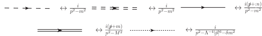
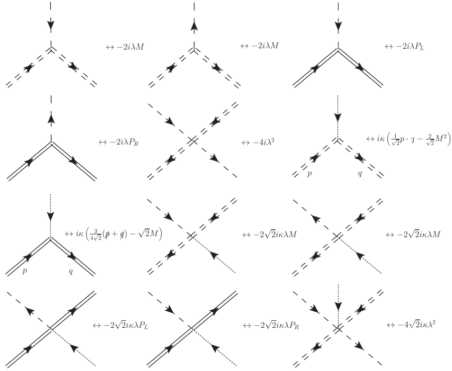
Figure 1: Feynman rules relevant for the calculation of the diagrams in fig. 2. The fields from the heavy chiral multiplet are denoted with double lines. Fermion lines are solid, and scalar graviton’s are dotted

4 Threshold corrections involving the heavy masses

As already explained, we are interested in evaluating the light scalar’s SUSY-breaking threshold corrections induced by the Lifshitz dynamics at high energy scales and involving the masses of the heavy fields. In this way we will be able to test whether these scalar-gravity-induced contributions are under control for a suitable choice of the Lifshitz scale $\Lambda$.

Since SUSY guarantees the nonrenormalization of the potential in the absence of the scalar graviton interactions ($\kappa\to 0$ limit), we need to calculate diagrams involving the latter. At one loop, all possible diagrams have no lines corresponding to heavy fields and thus will not give rise to any dependence on the heavy mass $M$ and will be ignored. The dominant diagrams contributing at two-loops are shown in fig. 2. Note that we have not included diagrams with scalar gravitons attached to the external light scalar legs through 3-point vertices. This is because such diagrams become proportional to the IR parameters, either the external momenta or the light mass $m$, and are thus subdominant. For similar reasons it is safe to ignore the counterterm diagrams corresponding to the one-loop divergences. For convenience, the external momentum can be put to zero for all diagrams.

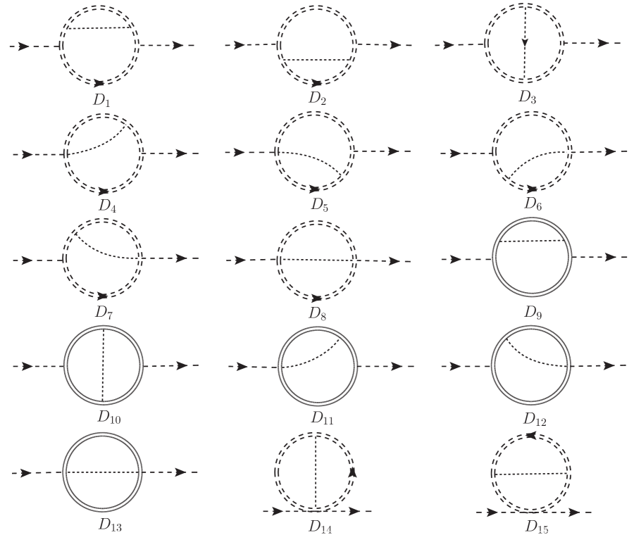
Figure 2: Two loop diagrams dominating the threshold corrections to the light scalar’s mass due to the heavy fields and the scalar graviton.

We have computed the diagrams using dimensional regularization in $D=4-2\epsilon$ dimensions, using the Feynman rules in fig. 1. All integrals can be reduced to the form

$$I[\alpha,\beta,\gamma,\rho,\sigma]=\int\frac{d^{D}kd^{D}l}{(2\pi)^{2D}}\frac{(l_{0})^{\rho}(|\vec{l}|)^{\sigma}}{[k^{2}-M^{2}]^{\alpha}[(k+l)^{2}-M^{2})]^{\beta}[(l^{2}-\Lambda^{-4}|\vec{l}|^{6}-\delta m^{2})]^{\gamma}},$$ (4.1)

with no $k$ dependence in the numerator. This is because the integrands obey the following relations,

$$k^{2}P[\alpha,\beta,\gamma]=P[\alpha-1,\beta,\gamma]+M^{2}P[\alpha,\beta,\gamma],$$

$$(l\cdot k)P[\alpha,\beta,\gamma]=\frac{1}{2}P[\alpha,\beta-1,\gamma]-\frac{l^{2}}{2}P[\alpha,\beta,\gamma]-\frac{1}{2}P[\alpha-1,\beta,\gamma],$$

which can be applied recursively. $P[\alpha,\beta,\gamma]$ here is defined as

$$P[\alpha,\beta,\gamma]\equiv\frac{1}{[k^{2}-M^{2}]^{\alpha}}\frac{1}{[(k+l)^{2}-M^{2}]^{\beta}}\frac{1}{[l^{2}-\Lambda^{-4}|\vec{l}|^{6}-M^{2}]^{\gamma}}.$$

In doing so, one arrives at some integrals with $\alpha=-1$, which can be obtained from $I[0,\beta,\gamma,\rho,\sigma]$ using the identity

$$I[-1,\beta,\gamma,\rho,\sigma]=I[0,\beta,\gamma,\rho+2,\sigma]-I[0,\beta,\gamma,\rho,\sigma+2]-M^{2}I[0,\beta,\gamma,\rho,\sigma].$$

A further symmetry property simplifying the calculations is

$$I[\alpha,\beta,\gamma,\rho,\sigma]=I[\beta,\alpha,\gamma,\rho,\sigma].$$

All the integrals needed for the calculation are obtained in appendix A, where analytic formulae are given for the dominant contributions in the limit of small $\Lambda$ and $x=\frac{\delta m^{2}}{M^{2}}$. These limits suit our goal of checking whether a small value of $\Lambda$ is able to suppress the contributions to soft masses due to loops of very heavy fields with masses $M\gg\Lambda$.

After using the above properties, the diagrams of fig. 2 have the following expressions in terms of the family of integrals $I[\alpha,\beta,\gamma,\rho,\sigma]$:

$$D_{1} =D_{2}=\frac{1}{2}i\kappa^{2}\lambda^{2}M^{2}\left(4M^{4}I[1,3,1,0,0]-5M^{2}I[0,3,1,0,0]\right.$$

$$-4M^{2}I[1,2,1,0,0]-4M^{2}I[1,3,1,0,2]+4M^{2}I[1,3,1,2,0]+2I[0,2,1,0,0]$$

$$+I[0,3,1,0,2]-I[0,3,1,2,0]+I[1,1,1,0,0]+2I[1,2,1,0,2]-2I[1,2,1,2,0]$$

$$\left.+I[1,3,1,0,4]-2I[1,3,1,2,2]+I[1,3,1,4,0]\right),$$

$$D_{3} =\frac{1}{2}iM^{2}\kappa^{2}\lambda^{2}\left(I[0,2,1,0,0]+2I[1,1,1,0,0]-4M^{2}I[1,2,1,0,0]+2I[1,2,1,0,2]\right.$$

$$-2I[1,2,1,2,0]+I[2,0,1,0,0]-4M^{2}I[2,1,1,0,0]+2I[2,1,1,0,2]-2I[2,1,1,2,0]$$

$$+4M^{4}I[2,2,1,0,0]-4M^{2}I[2,2,1,0,2]+I[2,2,1,0,4]+4M^{2}I[2,2,1,2,0]$$

$$\left.-2I[2,2,1,2,2]+I[2,2,1,4,0]\right),$$

$$D_{4} =D_{5}=D_{6}=D_{7}=2iM^{2}\kappa^{2}\lambda^{2}\left(-I[0,2,1,0,0]-I[1,1,1,0,0]+2M^{2}I[1,2,1,0,0]\right.$$

$$\left.-I[1,2,1,0,2]+I[1,2,1,2,0]\right),$$

$$D_{8} =8iM^{2}\kappa^{2}\lambda^{2}I[1,1,1,0,0],$$

$$D_{9} =-\frac{1}{8}i\kappa^{2}\lambda^{2}\left(32M^{6}I[1,3,1,0,0]-58M^{4}I[0,3,1,0,0]-16M^{4}I[1,2,1,0,0]\right.$$

$$+8M^{4}I[1,3,1,0,2]-8M^{4}I[1,3,1,2,0]-29M^{2}I[0,2,1,0,0]-14M^{2}I[1,1,1,0,0]$$

$$-8M^{2}I[1,2,1,0,2]+8M^{2}I[1,2,1,2,0]+63I[0,1,1,0,0]+9I[1,1,1,0,2]$$

$$\left.-9I[1,1,1,2,0]\right),$$

$$D_{10} =-\frac{1}{8}i\kappa^{2}\lambda^{2}\left(36I[0,1,1,0,0]+6M^{2}I[0,2,1,0,0]-18M^{2}I[1,1,1,0,0]+9I[1,1,1,0,2]\right.$$

$$-9I[1,1,1,2,0]-32M^{4}I[1,2,1,0,0]-12M^{2}I[1,2,1,0,2]+12M^{2}I[1,2,1,2,0]$$

$$\left.+16M^{6}I[2,2,1,0,0]+4M^{4}I[2,2,1,0,2]-4M^{4}I[2,2,1,2,0]\right),$$

$$D_{11} =D_{12}=i\kappa^{2}\lambda^{2}\left(12I[0,1,1,0,0]+4M^{2}I[0,2,1,0,0]+3I[1,1,1,0,2]-3I[1,1,1,2,0]\right.$$

$$\left.-8M^{4}I[1,2,1,0,0]-2M^{2}I[1,2,1,0,2]+2M^{2}I[1,2,1,2,0]\right),$$

$$D_{13} =-4i\kappa^{2}\lambda^{2}\left(2I[0,1,1,0,0]+2M^{2}I[1,1,1,0,0]+I[1,1,1,0,2]-I[1,1,1,2,0]\right),$$

$$D_{14} =-2i\kappa^{2}\lambda^{2}\left(2I[0,1,1,0,0]-2M^{2}I[1,1,1,0,0]+I[1,1,1,0,2]-I[1,1,1,2,0]\right),$$

$$D_{15} =\frac{1}{2}i\kappa^{2}\lambda^{2}\left(4M^{4}I[1,2,1,0,0]-5M^{2}I[0,2,1,0,0]-4M^{2}I[1,1,1,0,0]-4M^{2}I[1,2,1,0,2]\right.$$

$$+4M^{2}I[1,2,1,2,0]+2I[0,1,1,0,0]+I[0,2,1,0,2]-I[0,2,1,2,0]+I[1,0,1,0,0]$$

$$\left.+2I[1,1,1,0,2]-2I[1,1,1,2,0]+I[1,2,1,0,4]-2I[1,2,1,2,2]+I[1,2,1,4,0]\right),$$

the total being

$$-i\Sigma_{\phi}[p=0]= \frac{1}{8}i\kappa^{2}\lambda^{2}\Big{(}M^{4}(18I[0,3,1,0,0]+16I[1,2,1,0,0]-40I[1,3,1,0,2]$$

$$+40I[1,3,1,2,0]-16I[2,1,1,0,0]-20I[2,2,1,0,2]+20I[2,2,1,2,0])$$

$$+M^{2}(23I[0,2,1,0,0]+8I[0,3,1,0,2]-8I[0,3,1,2,0]$$

$$-68I[1,2,1,0,2]+68I[1,2,1,2,0]+8I[1,3,1,0,4]-16I[1,3,1,2,2]$$

$$+8I[1,3,1,4,0]+4I[2,0,1,0,0]+8I[2,1,1,0,2]-8I[2,1,1,2,0]$$ (4.2)

$$+4I[2,2,1,0,4]-8I[2,2,1,2,2]+4I[2,2,1,4,0])+5I[0,1,1,0,0]$$

$$+4I[0,2,1,0,2]-4I[0,2,1,2,0]+4I[1,0,1,0,0]-10I[1,1,1,0,2]$$

$$+10I[1,1,1,2,0]+4I[1,2,1,0,4]-8I[1,2,1,2,2]+4I[1,2,1,4,0]\Big{)}.$$

Before substituting the results of the integration in dimensional regularization, it is worth to dwell upon the the degree of divergence of the contributing integrals. The presence of Lifshitz propagators modifies the usual power counting, and if the integrals $I[\alpha,\beta,\gamma,\rho,\sigma]$ were to be computed with a cutoff regularization, the leading dependence on the cutoff $\Lambda_{\textrm{UV}}$ would be

$$I[\alpha,\beta,\gamma,\rho,\sigma]\sim\Lambda^{2+2\frac{\sigma}{3}}\Lambda_{\textrm{UV}}^{6-2\alpha-2\beta-2\gamma+\rho+\frac{\sigma}{3}}.$$ (4.3)

From this one can conclude that the divergences in $-i\Sigma_{\phi}[p=0]$ are at worst quadratic, which is an improvement with respect to the quartic divergences that ordinary scalar gravity would give rise to. Still, the dreaded quadratic divergences do not cancel and sneak back into the theory because of the hard SUSY breaking entailed by the scalar graviton interactions. However, as follows from eq. (4.3) and the $\kappa^{2}$ dependence in eq. (4.2), these divergences come with factors of $(\frac{\Lambda}{M_{P}})^{2}\Lambda^{2\frac{\sigma}{3}}$, so that they are strongly suppressed for $\Lambda\ll M_{P}$. Expression (4.3) is deduced for $z=3$, while higher $z$ lead to a higher power of $\Lambda$.

A similar suppression holds for the results in the limit of small $\Lambda$ in dimensional regularization, including the finite parts. Using the analytic formulae in § A, we obtain the following expression valid for $x=0$ in the limit of small $\Lambda$:

$$-i\Sigma_{\phi}[p=0] \sim\frac{i\kappa^{2}\lambda^{2}\Lambda^{2}M^{2}}{256\pi^{4}}\Big{\{}\frac{18}{\epsilon^{2}}-\frac{12}{\epsilon}\left(-3+3\gamma+\text{Log}\left[\frac{M^{4}\Lambda^{2}}{8\pi^{3}\mu^{6}}\right]\right)$$

$$+80-\pi^{2}+72\text{Log}[2\pi]+36\left(\gamma^{2}+\text{Log}[2]^{2}-2\gamma(1+\text{Log}[2\pi])\right.$$

$$\left.+\text{Log}[\pi]\text{Log}[4\pi]\right)+16\text{Log}\left[\frac{M^{2}\Lambda}{\mu^{3}}\right]\left(-3+3\gamma+\text{Log}\left[\frac{M^{2}\Lambda}{8\pi^{3}\mu^{3}}\right]\right)+O(\Lambda^{\frac{10}{3}}).$$

Despite the fact that some diagrams are IR divergent in the limit $x\rightarrow 0$ (those involving the integral $I[1,1,1,0,0]$, see appendix A), the final result is IR safe as expected for physical observables.

5 Conclusions

The main conclusion of our paper is that the combination of a supersymmetric matter sector and Hořava-Lifshitz gravity gives rise to interesting models, in which both Lorentz violation and SUSY breaking have a common origin and are controlled by a single dimensionless ratio,

$$\frac{\Delta c}{c}\propto\frac{\Lambda_{\textrm{HL}}^{2}}{M_{P}^{2}};~{}~{}~{}m^{2}_{\rm~{}SUSY~{}breaking}\propto\Lambda_{\textrm{UV}}^{2}\times\frac{\Lambda_{\textrm{HL}}^{2}}{M_{P}^{2}}.$$ (5.1)

The consideration of a very large ultraviolet scale, $\Lambda_{\textrm{UV}}\sim M_{P}$, and the requirement of a natural resolution to the gauge hierarchy problem then imply

$$\Lambda_{\textrm{HL}}\sim{\rm weak~{}scale}.$$ (5.2)

Supersymmetry in the matter sector also serves as a good argument for explaining why LV without the involvement of gravity is pushed to irrelevant operators.

To demonstrate our main point we took the simplest supersymmetric Wess-Zumino model with two chiral superfields, heavy and light, and coupled it to scalar gravity with Lifshitz scaling. A direct calculation in dimensional regularization of two-loop quantum corrections to the light scalar’s mass due to the gravitational interactions and the heavy fields revealed the universality of the $\Lambda_{\textrm{HL}}^{2}/M_{P}^{2}$ suppression. While the UV sensitivity of light masses remains, it is rendered harmless by the wide separation between the HL and Planck scales.

Our approach puts the gravitational force in a completely separate category from the rest of the interactions: it is not supersymmetric, violates Lorentz symmetry maximally, and acquires a Lifshitz scaling at relatively low energies (e.g. weak scale). If out of this one may eventually build a reliable theory of quantum gravity, it is a relatively modest theoretical price to pay.

Appendix A Evaluation of 2 loop integrals

All relevant two-loop diagrams can be written in terms of a family of 2-loop integrals with two heavy ordinary propagators and one Lifshitz propagator. We consider dimensional regularization in $D=4-2\epsilon$ dimensions. The family of integrals is given by

$$I[\alpha,\beta,\gamma,\rho,\sigma]=\int\frac{d^{D}kd^{D}l}{(2\pi)^{2D}}\frac{(l_{0})^{\rho}(|\vec{l}|)^{\sigma}}{[k^{2}-M^{2}]^{\alpha}[(k+l)^{2}-M^{2})]^{\beta}[(l^{2}-\Lambda^{-4}|\vec{l}|^{6}-\delta m^{2})]^{\gamma}}.$$

The usual power counting is modified in the presence of propagators of Lifshitz type. If one were to define the integrals by means of a cutoff regularization with cutoff $\Lambda_{C}$, the leading cutoff dependence would be

$$I[\alpha,\beta,\gamma,\rho,\sigma]\sim\Lambda^{2+2\frac{\sigma}{3}}\Lambda_{C}^{6-2\alpha-2\beta-2\gamma+\rho+\frac{\sigma}{3}}.$$

Thus the degree of divergence is lowered with respect to the one that would be obtained with ordinary propagators.

In the case in which all parameters $\alpha,\beta,\gamma,\rho,\sigma$ are greater than zero, we can reduce these integrals to a single one-dimensional complex integral applying the techniques in ref. [17] as follows. First, we apply the identities

$$\frac{1}{A^{\alpha}B^{\beta}}=\frac{\Gamma[\alpha+\beta]}{\Gamma[\alpha]\Gamma[\beta]}\int_{0}^{1}dx\frac{x^{\alpha-1}(1-x)^{\beta-1}}{[xA+(1-x)B]^{\alpha+\beta}},$$ (A.1)

$$\int\frac{d^{D}k}{(2\pi)^{D}}\frac{1}{[k^{2}-M^{2}]^{\lambda}}=\frac{i(-1)^{\lambda}}{2^{D}\pi^{D/2}}\frac{\Gamma\left[\lambda-\frac{D}{2}\right]}{\Gamma[\lambda]}(M^{2})^{\frac{D}{2}-\lambda}$$

to perform the integration in $k$. Applying eq. (A.1) again one is left with the following integral:

$$\int_{0}^{1}d\xi\,d\eta\,\int d^{D}l\,\frac{i(-1)^{\alpha+\beta}\Gamma[\alpha+\beta+\gamma-D/2]\xi^{\alpha-1}(1-\xi)^{\beta-1}\eta^{\gamma-1}(1-\eta)^{\alpha+\beta-D/2-1}l_{0}^{\rho}|\vec{l}|^{\sigma}}{2^{2D}\pi^{3D/2}\Gamma[\alpha]\Gamma[\beta]\Gamma[\gamma]([\eta-(1-\eta)\xi(1-\xi)][l^{2}-\tilde{\Lambda}^{-4}|\vec{l}|^{6}-\tilde{M}^{2}])^{\alpha+\beta+\gamma-D/2}},$$

$$\tilde{\Lambda}=\Lambda\left(\frac{\eta}{\eta-(1-\eta)\xi(1-\xi)}\right)^{-\frac{1}{4}},$$

$$\tilde{M}^{2}=\frac{M^{2}(\eta x-(1-\eta))}{\eta-(1-\eta)\xi(1-\xi)},$$ (A.2)

where we defined

$$x\equiv\frac{\delta m^{2}}{M^{2}}.$$

In order to perform the $l$ integral, we use the propagator representation

$$\frac{1}{A^{c}}=\frac{i^{c}\lambda^{c-1}}{\Gamma[c]}\int_{0}^{\infty}d\lambda e^{-i\lambda A}.$$ (A.3)

The $l^{0}$ integral can be computed after a proper contour deformation, and is given by

$$\int_{-\infty}^{\infty}dl_{0}l_{0}^{\rho}e^{-i\lambda l_{0}^{2}}=\!-\frac{(i\!-\!1)^{\rho+1}}{2^{\frac{\rho+1}{2}}}\int_{\!-\infty}^{\infty}dyy^{\rho}e^{-\lambda y^{2}}=-\frac{(-1)^{3/4}}{2}(1+(-1)^{\rho})e^{\frac{3i\pi\rho}{4}}\lambda^{-1/2-\rho/2}\Gamma\left[\frac{1+\rho}{2}\right].$$

The integral along $d^{3}\vec{l}$ can be expressed in terms of hypergeometric functions. We are interested in threshold effects from very heavy fields mediated by the scalar gravity interactions, which explicitly break supersymmetry and hence violate the nonrenormalization of the superpotential. For this reason we are interested in the limit of $M\gg\Lambda$ (very heavy thresholds). In this limit the dominant contribution to the integral over $d^{3}\vec{l}$ is

$$\frac{2\pi^{\frac{D-1}{2}}}{\Gamma[\frac{D-1}{2}]}\int_{0}^{\infty}d|\vec{l}||\vec{l}|^{D-2+\sigma}e^{i\lambda(|\vec{l}|^{2}+\tilde{\Lambda}^{-4}|\vec{l}|^{6}+\tilde{M}^{2})}=$$

$$=-\frac{1}{6}(-1)^{11/12}\lambda^{\frac{1}{6}(-D-\sigma+1)}\Lambda^{\frac{2}{3}(D+\sigma-1)}\Gamma\left[\frac{1}{6}(D+\sigma-1)\right]e^{\frac{1}{12}i\pi(D+\sigma)+i\lambda M^{2}}+O(\Lambda^{\frac{2}{3}+D+\sigma}).$$

In this limit one may perform the integral over $\lambda$; also, it is useful to rewrite the part of the denominator in eq. (A.2) involving $\xi,\eta$ as a product of factors, by using the Mellin-Barnes identity

$$\frac{1}{(A+B)^{c}}=\frac{1}{2\pi i\Gamma[c]}\int_{-i\infty}^{i\infty}dz\frac{A^{z}\Gamma[c+z]\Gamma[-z]}{B^{c+z}}.$$

Here the contour is taken between the left and right handed poles of the Gamma functions –the left poles are those corresponding to the factors $\Gamma[z+\dots]$, and the right poles those of the factors $\Gamma[-z+\dots]$. In this way one gets the following representation of the integral $I[\alpha,\beta,\gamma,\rho,\sigma]$:

$$I[\alpha,\beta,\rho,\sigma]=\int_{-i\infty}^{i\infty}dz\int_{0}^{1}d\xi\,d\eta\,\frac{(-1)^{\gamma}i^{\rho-D}(1+(-1)^{\rho})\Gamma[\frac{1}{6}(D+\sigma-1)]}{2^{2D}\pi^{D+\frac{1}{2}}6\Gamma[\alpha]\Gamma[\beta]\Gamma[\gamma]\Gamma[\frac{D-1}{2}]}\Gamma[-z]\Gamma\left[\frac{1+\rho}{2}+z\right]\times$$

$$\times\Gamma\left[-\frac{1}{3}+\alpha+\beta+\gamma-\frac{2D}{3}-\frac{\rho}{2}-\frac{\sigma}{6}\right]\Lambda^{\frac{2(D-1+\sigma)}{3}}M^{\frac{1}{3}(2-6\alpha-6\beta-6\gamma+4D+3\rho+\sigma)}\times$$

$$\times\frac{\xi^{\alpha-1}(1-\xi)^{\beta-1}\eta^{\gamma-1+z-\frac{1}{6}(D+\sigma-1)}(1-\eta)^{\alpha+\beta-\frac{D}{2}-1}(x\eta-(1-\eta))^{\frac{1}{6}(2-6\alpha-6\beta-6\gamma+4D+3\rho+\sigma)}}{[-(1-\eta)\xi(1-\xi)]^{\frac{1+\rho}{2}+z}}.$$

The integral in the parameters $\xi,\eta$ can be expressed in terms of Gamma functions, leaving only a one dimensional contour integral:

$$I[\alpha,\beta,\rho,\sigma]=\int_{-i\infty}^{i\infty}dz\,\frac{i^{1-\rho}(-1)^{\alpha+\beta+\gamma}4^{-1-D}(1+(-1)^{\rho})\Gamma[\frac{1}{6}(D+\sigma\!-\!1)]}{3\pi^{D+\frac{3}{2}}\Gamma[\alpha]\Gamma[\beta]\Gamma[\gamma]\Gamma[\frac{D-1}{2}]\Gamma[\alpha+\beta-\rho-2z-1]}\Gamma\left[\!-\frac{1}{2}+\alpha\!-\frac{\rho}{2}\!-z\right]\times$$

$$\times\Gamma\left[-\frac{1}{2}+\beta-\frac{\rho}{2}-z\right]\Gamma\left[-\frac{1}{2}+\alpha+\beta-\frac{D}{2}-\frac{\rho}{2}-z\right]\Gamma[-z]\Gamma\left[\frac{1+\rho}{2}+z\right]\times$$

$$\times\Gamma\left[\frac{1}{6}-\frac{D}{6}+\gamma-\frac{\sigma}{6}+z\right]\Lambda^{\frac{2(D-1+\sigma)}{3}}M^{\frac{1}{3}(2-6\alpha-6\beta-6\gamma+4D+3\rho+\sigma)}x^{\frac{1}{6}(-1+D-6\gamma+\sigma-6z)}.$$

Again, the contour integral runs between the right and left poles of the Gamma functions. The singularities in $D=4$ come from either z-independent Gamma functions or when the integration contour is pinched between poles that approach as $D\rightarrow 4$. The latter can be isolated by appropriately deforming the integration contour, so that $I[\alpha,\beta,\gamma,\rho,\sigma]$ can be expressed as a sum over residues over some of the poles pinching the integration contour plus another line integral free of singularities as $D\rightarrow 4$, for which the latter limit may be safely taken.

As an example, let’s evaluate $I[1,1,1,0,0]$. From eq. (4.1), one can see that the left-handed poles in $z$ of the Gamma functions sit at $\{-\frac{1}{2}-k,\,-\frac{1}{2}-\frac{\epsilon}{3}-k\},\,k=0,1,2,\dots$, while the right handed poles are at $\{\frac{1}{2}+k,\,-\frac{1}{2}+\epsilon+k\},\,k=0,1,2,\dots$. Thus there is a pinch singularity when $D\rightarrow 4$ ($\epsilon\rightarrow 0$) as the contour is trapped between the poles at $z=-\frac{1}{2}$ and $z=-\frac{1}{2}+\epsilon$. The contour can be deformed as the sum of a vertical line to the left of the $z=-\frac{1}{2}-\frac{\epsilon}{3}$ pole plus a sum of residues over $z=-\frac{1}{2}-\frac{\epsilon}{3}$ and $z=-\frac{1}{2}$. The line integral is finite for $D\rightarrow 4$ and can be evaluated closing the contour on the left and summing over the residues of the poles inside the contour; the sum converges very quickly and we choose to approximate it by the first terms corresponding to the poles closer to the origin, which is equivalent to an expansion in $x$; in this case, the first term is already of order $x^{2}$ and we will neglect it. We are left just with the residues of the poles giving rise to the singularity, that is

$$I[1,1,1,0,0]=\Lambda^{2}\left\{\frac{1}{512\pi^{4}\epsilon^{2}}-\frac{1}{1536\pi^{4}\epsilon}\left(\log\left(\frac{\Lambda^{4}M^{8}x^{4}}{16384\pi^{6}}\right)+6(\gamma-2)\right)\right.$$

$$\!+\!\frac{1}{27648\pi^{4}}\Big{[}48\log(\Lambda)\left(\log\left(\frac{\Lambda M^{4}x^{2}}{128\pi^{3}}\right)-6\right)+96\log(M)\left(\log\left(\frac{x^{2}}{128\pi^{3}}\right)+3\gamma-6\right)$$

$$+192\log^{2}(M)+144\gamma\log(\Lambda x)+12\log(x)(\log(x)-4(3+\log(16)+3\log(\pi)))-19\pi^{2}$$

$$+12\left(30+9\log^{2}(\pi)+6(6\right.$$

$$\left.+\log(128))\log(\pi)+\log(2)(60+37\log(2))\right)+36\gamma(3\gamma-2(6+\log(128)+3\log(\pi)))\Big{]}\Big{\}},$$

where $\gamma$ is the Euler constant. In a similar way, results for all the integrals needed for the computation follow. Where appropriate, we have computed line integrals which are finite at $D=4$ by closing contours and summing over residues. These sums are dominated by the residues of the poles closest to the origin, and we give the corresponding analytic expressions –in fact, the residues of these poles involve powers of $x=\delta m^{2}/M^{2}$ that increase with the distance to the origin, so that the formulae below correspond to the lowest terms in an $x$ expansion. Thus, in the previous formula and the ones that follow, equalities are understood up to higher orders in $\Lambda$ and $x$.

$$I[1,1,1,2,0]=\Lambda^{2}M^{2}\Big{\{}\frac{x+12}{1024\pi^{4}\epsilon^{2}}+\frac{1}{1536\pi^{4}\epsilon}\Big{[}\!-24\log\left(\Lambda M^{2}\right)-2x\log\left(\Lambda M^{2}x\right)-3\gamma(x+12)$$

$$+x(5+\log(128)+3\log(\pi))+60+36\log(2\pi)\Big{]}+\frac{1}{55296\pi^{4}}\Big{[}576(3\gamma-5)\log\left(\Lambda M^{2}\right)$$

$$+12\left(-2x\log(x)\left(-4\log\left(\Lambda M^{2}\right)+7+\log(256)\right)+4\log\left(\Lambda M^{2}\right)\left((x+12)\log\left(\Lambda M^{2}\right)\right.\right.$$

$$\left.\left.-x(5\!+\!\log(128))\!-\!12\log\left(8\pi^{3}\right)\right)+12x(\gamma\!-\!\log(\pi))\log\left(\Lambda M^{2}x\right)+x\log^{2}(x)\right)+108\gamma^{2}(x+12)$$

$$-\pi^{2}(19x+36)+12\left(x\left(32+9\log^{2}(\pi)+6(5+\log(128))\log(\pi)+\log(2)(58+37\log(2))\right)\right.$$

$$\left.\!+\!12\left(38\!+\!9\log^{2}(2)\!+\!30\log(2\pi)+3\log(\pi)\log\left(64\pi^{3}\right)\right)\right)-72\gamma(x(5+\log(128)+3\log(\pi))+60$$

$$+36\log(2\pi))\Big{]}\Big{\}},$$

$$I[1,1,1,0,2]=(xM^{2}\Lambda^{10})^{1/3}\Big{\{}\frac{\Gamma\left(-\frac{1}{3}\right)\Gamma\left(\frac{5}{6}\right)}{384\pi^{9/2}\epsilon}+\frac{1}{1152\pi^{9/2}}\Big{[}\Gamma\left(-\frac{1}{3}\right)\Gamma\left(\frac{5}{6}\right)\left(\log\left(\frac{256\pi^{6}}{\Lambda^{4}M^{8}x}\right)\right.$$

$$\left.-\frac{\pi}{\sqrt{3}}-6\gamma+9\right)\Big{]}-\frac{(x-84)\Gamma\left(-\frac{7}{6}\right)\Gamma\left(-\frac{1}{3}\right)}{13824\left(\sqrt[3]{2}\sqrt{3}\pi^{7/2}\sqrt[3]{x}\right)}-\frac{x\Gamma\left(-\frac{4}{3}\right)\Gamma\left(\frac{5}{6}\right)}{4608\pi^{9/2}}\Big{\}},$$

$$I[1,2,1,4,0]=(\Lambda M)^{2}\Big{\{}\frac{3(x+4)}{1024\pi^{4}\epsilon^{2}}-\frac{1}{1024\pi^{4}\epsilon}(x+4)\left(\log\left(\frac{\Lambda^{4}M^{8}}{64\pi^{6}}\right)+6\gamma-8\right)$$

$$+\frac{1}{6144\pi^{4}}\Big{[}\!-\!256\log(\Lambda)+4\left(4(x+4)\left(\log\left(\frac{\Lambda^{4}}{64\pi^{6}}\right)+6\gamma-8\right)\log(M)+16(x+4)\log^{2}(M)\right.$$

$$\left.+\log\left(\frac{\pi^{3}}{\Lambda^{2}}\right)(-2(x+4)\log(\Lambda)-6\gamma(x+4)+x(8+\log(64)+3\log(\pi))+12\log(4\pi))\right),$$

$$+36\gamma^{2}(x+4)-\pi^{2}(x+4)-24\gamma(x+4)(4+\log(8))+12\log(2)(8x+(x+4)\log(8))$$

$$+32(3x+2(7+\log(64)+6\log(\pi)))\Big{]}\},$$

$$I[1,2,1,0,4]=\frac{\Lambda^{\frac{14}{3}}}{M^{\frac{2}{3}}}\Big{\{}\frac{(x-60)\Gamma\left(-\frac{2}{3}\right)}{13122\pi^{2}\Gamma\left(\frac{5}{3}\right)\Gamma\left(\frac{11}{3}\right)}+\frac{x^{2/3}(x+20)\Gamma\left(-\frac{5}{3}\right)\Gamma\left(\frac{7}{6}\right)}{9216\pi^{9/2}}\Big{\}},$$

$$I[1,2,1,2,2]=\Lambda^{\frac{10}{3}}M^{\frac{2}{3}}\frac{(x-12)\Gamma\left(-\frac{1}{3}\right)}{3888\pi^{2}\Gamma\left(\frac{1}{3}\right)\Gamma\left(\frac{7}{3}\right)},$$

$$I[1,3,1,2,0]=\frac{\Lambda^{2}}{M^{2}}\Big{\{}-\frac{1}{256\pi^{4}\epsilon}+\frac{\log\left(\frac{\Lambda^{4}M^{8}}{64\pi^{6}}\right)+6\gamma-5}{768\pi^{4}}+\frac{x(-6\log(x)+1+6\log(4))}{27648\pi^{4}}\Big{\}},$$

$$I[1,3,1,0,2]=\left(\frac{\Lambda}{M}\right)^{10/3}\Big{\{}-\frac{\sqrt[3]{x}(9x+80)\Gamma\left(-\frac{4}{3}\right)\Gamma\left(\frac{5}{6}\right)}{138240\pi^{9/2}}+\frac{175(2x+39)\Gamma\left(\frac{5}{3}\right)}{118098\pi^{2}\Gamma\left(\frac{10}{3}\right)\Gamma\left(\frac{16}{3}\right)}\Big{\}},$$

$$I[2,2,1,2,0]=\frac{\Lambda^{2}}{M^{2}}\Big{\{}-\frac{x-6x\log(2)+3x\log(x)+36}{13824\pi^{4}}\Big{\}},$$

$$I[2,2,1,0,2]=\left(\frac{\Lambda}{M}\right)^{\frac{10}{3}}\Big{\{}-\frac{\sqrt[3]{x}(3x+20)\Gamma\left(-\frac{4}{3}\right)\Gamma\left(\frac{5}{6}\right)}{34560\pi^{9/2}}+\frac{35(25x+312)\Gamma\left(\frac{2}{3}\right)}{354294\pi^{2}\Gamma\left(\frac{10}{3}\right)\Gamma\left(\frac{16}{3}\right)}\Big{\}},$$

$$I[1,2,1,2,0]=\Lambda^{2}\Big{\{}\frac{3}{512\pi^{4}\epsilon^{2}}+\frac{\log\left(\frac{64\pi^{6}}{\Lambda^{4}M^{8}}\right)-6\gamma+6}{512\pi^{4}\epsilon}$$

$$+\frac{1}{3072\pi^{4}}\Big{[}16\log\left(\Lambda M^{2}\right)\left(\log\left(\Lambda M^{2}\right)+3\gamma-3-3\log(2\pi)\right)-\pi^{2}+36\gamma(\gamma-2(1+\log(2\pi)))$$

$$+36(2+\log(2\pi)(2+\log(2\pi)))\Big{]}+\frac{x\left(\log\left(\frac{x}{4}\right)-1\right)}{1536\pi^{4}}\Big{\}},$$

$$I[1,2,1,0,2]=\left(\frac{\Lambda^{10}}{M^{4}}\right)^{\frac{1}{3}}\Big{\{}-\frac{10(x+42)\Gamma\left(-\frac{4}{3}\right)}{59049\pi^{2}\Gamma\left(\frac{7}{3}\right)\Gamma\left(\frac{13}{3}\right)}+\frac{\sqrt[3]{x}(x+16)\Gamma\left(-\frac{4}{3}\right)\Gamma\left(\frac{5}{6}\right)}{9216\pi^{9/2}}\Big{\}},$$

$$I[1,3,1,4,0]=\Lambda^{2}\Big{\{}-\frac{1}{512\pi^{4}\epsilon}+\frac{\log\left(\frac{\Lambda^{4}M^{8}}{64\pi^{6}}\right)+6\gamma-6}{1536\pi^{4}}+\frac{x\log\left(\frac{4}{x}\right)}{1536\pi^{4}}\Big{\}},$$

$$I[1,3,1,0,4]=\frac{\Lambda^{\frac{14}{3}}}{M^{\frac{8}{3}}}\Big{\{}\frac{5(7x-132)\Gamma\left(\frac{4}{3}\right)}{39366\pi^{2}\Gamma\left(\frac{8}{3}\right)\Gamma\left(\frac{14}{3}\right)}-\frac{x^{2/3}(9x+100)\Gamma\left(-\frac{5}{3}\right)\Gamma\left(\frac{7}{6}\right)}{138240\pi^{9/2}}\Big{\}},$$

$$I[1,3,1,2,2]=\frac{\Lambda^{\frac{10}{3}}}{M^{\frac{4}{3}}}\Big{\{}\frac{(5x+84)\Gamma\left(-\frac{4}{3}\right)\Gamma\left(\frac{5}{3}\right)}{11664\sqrt{3}\pi^{3}\Gamma\left(\frac{10}{3}\right)}-\frac{x^{4/3}\Gamma\left(-\frac{4}{3}\right)\Gamma\left(\frac{5}{6}\right)}{4608\pi^{9/2}}\Big{\}},$$

$$I[2,2,1,4,0]=\Lambda^{2}\Big{\{}\frac{3}{256\pi^{4}\epsilon^{2}}+\frac{\log\left(\frac{64\pi^{6}}{\Lambda^{4}M^{8}}\right)-6\gamma+5}{256\pi^{4}\epsilon}+\frac{1}{1536\pi^{4}}\Big{[}40\log\left(\frac{4}{\Lambda}\right)$$

$$+16\log(\Lambda)(\log(\Lambda)+3\gamma-3\log(2\pi))+16(4\log(\Lambda)+6\gamma-5-6\log(2\pi))\log(M)$$

$$+64\log^{2}(M)-\pi^{2}+4(15+\log(2)(\log(512)-5)+3\log(\pi)(5+\log(64)+3\log(\pi)))$$

$$+12\gamma(3\gamma-5-6\log(2\pi))\Big{]}-\frac{x}{768\pi^{4}}\Big{\}},$$

$$I[2,2,1,0,4]=\frac{\Lambda^{\frac{14}{3}}}{M^{\frac{8}{3}}}\Big{\{}\frac{10(33-4x)\Gamma\left(-\frac{2}{3}\right)}{177147\pi^{2}\Gamma\left(\frac{8}{3}\right)\Gamma\left(\frac{14}{3}\right)}-\frac{x^{2/3}(3x+25)\Gamma\left(-\frac{5}{3}\right)\Gamma\left(\frac{7}{6}\right)}{34560\pi^{9/2}}\Big{\}},$$

$$I[2,2,1,2,2]=\frac{\Lambda^{\frac{10}{3}}}{M^{\frac{4}{3}}}\Big{\{}\frac{(x-21)\Gamma\left(\frac{11}{6}\right)}{2430\sqrt[3]{2}\pi^{5/2}\Gamma\left(\frac{10}{3}\right)}-\frac{x^{4/3}\Gamma\left(-\frac{4}{3}\right)\Gamma\left(\frac{5}{6}\right)}{4608\pi^{9/2}}\Big{\}}.$$

Except for $I[1,1,1,0,0]$, the previous integrals have a well defined limit when $x\rightarrow 0$. In the case $\alpha=0$ (or equivalently $\beta=0$), with the rest of parameters staying positive, the two-loop integral factorizes in one-loop integrals, and the $l$ integral can be performed using eq. (A.3) as before. Doing a series expansion in $\Lambda$ and keeping the lowest order, one gets

$$I[0,\beta,\gamma,\rho,\sigma]= I[\beta,0,\gamma,\rho,\sigma]=\frac{i^{2\gamma+\rho}(1+(-1)^{\rho})}{3\cdot 2^{2+D}\pi^{D/2}\Gamma[\beta]\Gamma[\gamma]}\Gamma\Big{[}\beta\!-\!\frac{D}{2}\Big{]}\Gamma\Big{[}\frac{1+\rho}{2}\Big{]}\Gamma\Big{[}\frac{1}{6}(\!-\!1+D+\sigma)\Big{]}\times$$

$$\times\Gamma\Big{[}\frac{1}{6}(-2-D+6\gamma-3\rho-\sigma)\Big{]}\Lambda^{\frac{2}{3}(-1+D+\sigma)}M^{\frac{1}{3}(D-2\beta)}\delta m^{\frac{1}{3}(2+D-6\gamma+3\rho+\sigma)}.$$

In the case $x=0$, the $l$ integral is of the tadpole type and it vanishes in dimensional regularization, so that

$$I[0,\beta,\gamma,\rho,\sigma]|_{x=0}=0.$$

References

• [1] P. Horava, Phys.Rev. D79, 084008 (2009), 0901.3775.
• [2] M. Pospelov and Y. Shang, Phys.Rev. D85, 105001 (2012), 1010.5249.
• [3] S. Groot Nibbelink and M. Pospelov, Phys.Rev.Lett. 94, 081601 (2005), hep-ph/0404271.
• [4] P. A. Bolokhov, S. Nibbelink Groot, and M. Pospelov, Phys.Rev. D72, 015013 (2005), hep-ph/0505029.
• [5] M. Pospelov and M. Romalis, Phys.Today 57N7, 40 (2004).
• [6] T. Jacobson, S. Liberati, and D. Mattingly, Annals Phys. 321, 150 (2006), astro-ph/0505267.
• [7] D. Colladay and V. A. Kostelecky, Phys.Rev. D55, 6760 (1997), hep-ph/9703464.
• [8] P. A. Bolokhov and M. Pospelov, Phys.Rev. D77, 025022 (2008), hep-ph/0703291.
• [9] M. M. Anber and J. F. Donoghue, Phys.Rev. D83, 105027 (2011), 1102.0789.
• [10] G. Bednik, O. Pujolas, and S. Sibiryakov, (2013), 1305.0011.
• [11] R. Iengo, J. G. Russo, and M. Serone, JHEP 0911, 020 (2009), 0906.3477.
• [12] I. Kimpton and A. Padilla, JHEP 1304, 133 (2013), 1301.6950.
• [13] D. Blas, O. Pujolas, and S. Sibiryakov, JHEP 1104, 018 (2011), 1007.3503.
• [14] S. Mukohyama, Class.Quant.Grav. 27, 223101 (2010), 1007.5199.
• [15] T. Griffin, P. Horava, and C. M. Melby-Thompson, JHEP 1205, 010 (2012), 1112.5660.
• [16] T. P. Sotiriou, J.Phys.Conf.Ser. 283, 012034 (2011), 1010.3218.
• [17] V. Smirnov, (2006), Feynman integral calculus.