Simultaneous Transmission and Reception: Algorithm, Design and System Level Performance

Abstract

Full Duplex or Simultaneous transmission and reception (STR) in the same frequency at the same time can potentially double the physical layer capacity. However, high power transmit signal will appear at receive chain as echoes with powers much higher than the desired received signal. Therefore, in order to achieve the potential gain, it is imperative to cancel these echoes. As these high power echoes can saturate low noise amplifier (LNA) and also digital domain echo cancellation requires unrealistically high resolution analog-to-digital converter (ADC), the echoes should be cancelled or suppressed sufficiently before LNA. In this paper we present a closed-loop echo cancellation technique which can be implemented purely in analogue domain. The advantages of our method are multiple-fold: it is robust to phase noise, does not require additional set of antennas, can be applied to wideband signals and the performance is irrelevant to radio frequency (RF) impairments in transmit chain. Next, we study a few protocols for STR systems in carrier sense multiple access (CSMA) network and investigate MAC level throughput with realistic assumptions in both single cell and multiple cells. We show that STR can reduce hidden node problem in CSMA network and produce gains of up to 279% in maximum throughput in such networks. Moreover, at high traffic load, the gain of STR system can be tremendously large since the throughput of non-STR system is close to zero at heavy traffic due to severe collisions. Finally, we investigate the application of STR in cellular systems and study two new unique interferences introduced to the system due to STR, namely BS-BS interference and UE-UE interference. We show that these two new interferences will hugely degrade system performance if not treated appropriately. We propose novel methods to reduce both interferences and investigate the performances in system level. We show that BS-BS interference can be suppressed sufficiently enough to be less than thermal noise power, and with favorable UE-UE channel model, capacities close to double are observed both in downlink (DL) and uplink (UL). When UE-UE interference is larger than DL co-channel interferences, we propose a simple and “non-cooperative” technique in order to reduce UE-UE interference.

I Introduction

Currently deployed wired and wireless communication systems employ half duplex. Namely, either frequency division duplex (FDD) or time division duplex (TDD) has been used for separate transmission and reception. In FDD and TDD, transmitted signal does not interfere with received signal due to orthogonal use of time/frequency resources for transmission and reception. Since two orthogonal channels are needed in half duplex systems, twice of time and/or frequency resources are required in half duplex compared to full duplex systems. It is clear that the capacity can be doubled by simultaneous transmission and reception in the same frequency at the same time.

I-A Benefits of Full Duplex

STR or full duplex systems not only improve the physical layer capacity but also provide other important benefits in layers beyond physical layer [1]. For example, STR can reduce or completely eliminate hidden node problem which is typical issue in CSMA networks such as wireless local area networks (WLAN). When a node receives a packet designated to it and meanwhile has a packet to transmit, by having STR capability it can transmit the packet while receiving the designated packet. This not only provides twice throughput but also enables hidden nodes to better detect active nodes in their neighborhoods. On the other hand, when the node has no packet to send, it can transmit a dummy signal so that any hidden node can detect the activity in its vicinity and realize that the channel is in use.

Another benefit of STR is significant reduction in end-to-end delay in multi-hop networks [1]. In half duplex systems, each node can start transmission of a packet to the next node only when it is fully received from the previous node in network. Therefore, the end-to-end delay is equal to packet duration multiplied by the number of hops. However, when STR is employed, a node can forward a packet while receiving it, and consequently the end-to-end delay in STR systems can be just a bit longer than the packet duration. This will be a huge advantage over half duplex systems especially as the number of hops grows. Meanwhile, the forwarded packet to next node can play a role of implicit acknowledgement (ACK) to previous node as well.

Interesting application of STR includes channel sensing in cognitive radio systems [1]. In cognitive radios, active secondary users have to release the spectrum when primary users start their transmissions. Without STR capability, it is a challenge for secondary users to detect activity of primary users while they are using the spectrum for their own communications. However, STR enabled secondary users can scan the activities of primary users frequently (even as they transmit) and stop their transmissions immediately once they detect primary users’ transmissions.

Likewise, STR makes the device discovery easier in device-to-device (D2D) systems. This is due to the fact that in D2D systems, when user equipment (UE) has STR capability, it can discover neighboring UEs easily by monitoring UL signals from proximate UEs without stopping its own UL transmission.

It is interesting to note that STR techniques can be used for interference cancellation in co-existence of multiple radios in the same device. Multiple radios such as WLAN, Bluetooth, GPS receiver, 2G and 3G cellular transceivers are put into the same device particularly a small handheld device type [2]. Although those radios operate at different RF carriers, due to proximity of transceivers in the same device, they can still interfere with each other. This interference can be treated as echo since the transmitted signal from a radio is arrived at other radios in the same device. Hence, by using the proposed technique in this paper, the co-existence issues in the same device can be resolved.

Multiband support requires large number of switched duplexers in FDD, resulting in quite complicated RF architecture, increased cost and form factor [3], [4]. Multiple input multiple output (MIMO) and carrier aggregation techniques aggravate the situation. However, by STR techniques duplexer free systems are possible by cancelling transmitted signal appeared at receive band.

I-B Prior Arts and Proposed Method

Despite all the advantages mentioned, implementation of STR has its own challenges. The main difficulty in STR system is echo cancellation at receive chain. The strongest echo is introduced to the system when transmitted signal is leaked into receive chain through circulator. This causes a large interference to the desired received signal as the echo power level is much higher than desired received signal. For example, with 46 dBm output power at power amplifier (PA), assuming 25 dB isolation at circulator, the echo power will be 21 dBm. In addition to the aforementioned echoes, echoes can be caused by impedance mismatch at antenna. Besides, transmitted signal can bounce off objects such as buildings and mountains, and return to the antenna as echoes at receive chain. Hence, without echo cancellation, the received signal cannot be decoded. Furthermore, in order to avoid saturation at LNA and high resolution ADC, echo cancellation should be performed before LNA. Therefore, it is imperative to cancel echoes in analogue domain in order for STR systems to be commercially deployable.

An off-the-shelf hardware [5] is available for RF interference cancellation in analogue and can be used for echo cancellation in RF. However, it is a narrowband interference canceller and performs interference cancellation by adjusting phase and magnitude of interference. Thus, the performance of echo cancellation in wideband signals is very limited. In [1] about 20 dB echo suppression is reported for 5 MHz IEEE 802.15.4 signals. In addition, this narrowband interference canceller can create higher sidelobe power than in-band interference power [1].

An STR implementation in analogue assuming separate transmit and receive antennas was reported in [3] claiming 37 dB suppression by the RF echo canceller itself. Recently, [6] presented an open-loop technique for full duplex MIMO. A hardware based experiment shows 50 dB of echo suppression. In [1], the echo cancellation using transmit beamforming is studied. This technique uses two transmit antennas and one receive antenna. The additional two transmit antennas create a null toward receive antenna, resulting in reduced echo power at receive chain. However, the transmitted signal is not omni-directionally transmitted due to the transmit beamforming. When the intended receiver is located in the null direction, signal-to-noise power ratio (SNR) loss is inevitable. Additionally, the transmit beamforming is narrowband beamforming. Thus, it is not suitable for wideband signal. Since this technique needs separate transmit and receive antenna set, increased form factor is unavoidable. Nonetheless, the echo suppression of 20 $\sim$ 30 dB by this technique is not promising. However, with the aids from digital baseband cancellation and the narrowband noise canceller [5], the imperfect prototype achieves 1.84 times of throughput compared to half duplex system throughput. A scalable design to MIMO using extra antennas with special placement antennas is proposed in [7]. In [8], assuming variable delay line, one-tap echo canceller is suggested. It is shown that 45 dB suppression of echo is achieved by using heuristic approach in adaptive parameter adjustment. The throughput measurements in [8] show 111% gain in downlink.

Another prior work [9] proposed to cancel echo before LNA. Firstly, to avoid saturation at LNA, separate transmit and receive antennas with large displacement are used. Various antenna orientations are investigated in [10]. The receiver estimates the echo channel at every subcarrier using OFDM signal. Using another transmit radio chain, an echo cancelling OFDM signal is generated based on the estimated channels of echo path and the additional radio, and added to the receive chain before LNA. The measured echo cancellation is about 31 $\sim$ 32 dB in [9] and 24 dB in [10]. This type of open-loop technique is directly sensitive to impairments as it relies on high accurate echo channel estimation. Since the suppression in this case is not sufficient to realize the full duplex gain, other mechanisms such as digital domain cancellation and separate transmit/receive antenna have to be incorporated.

Without using additional antennas, we propose an adaptive echo cancellation technique that can be implemented in analogue domain for wideband signals. The proposed technique is a closed-loop technique which provides more robustness to impairments than open-loop techniques. Furthermore, the proposed technique is scalable to any MIMO system.

I-C Applications to Multicell Communications

As mentioned earlier, with perfect echo cancellation, STR systems can achieve the doubled capacity especially in isolated links such as point-to-point communications and wireless backhaul. However, in cellular systems the situation is different. In addition to the regular co-channel interference present in half duplex systems, namely base station (BS) to UE and UE to BS interferences, there are two unique and serious interferences caused by system operation in full duplex mode: one is BS-BS and the other is UE-UE.

On one hand, due to STR at BSs, neighboring BSs’ DL signals interfere with desired UL signal at home BS. This is called BS-BS interference and is extremely severe. Firstly, unlike BS to UE channel (downlink or uplink), BS-to-BS channel is closer to line-of-sight (LoS) with much smaller path loss. Secondly, the transmit power and antenna gain at BS is much larger than those of UE. Hence, the interferences from neighboring BSs to home BS easily dominate desired weak UL signal. Hence, without cancelling BS-BS interferences, UL communication is impossible. In this paper we suggest a solution for BS-BS interferences and provide system level evaluations for STR systems with and without BS-BS interference cancellation.

On the other hand, in STR systems, UL signal transmitted by a UE creates interference to DL signals received at other UEs i.e., DL signal will be corrupted by proximate UL signals. This is called UE-UE interference and results in loss of DL capacity. Unfortunately, with simple transceiver and omni-directional single antenna at UE, no fancy transmit and receive beamforming can be utilized in UE to handle UE-UE interference. Therefore, one option to confront UE-UE interference is to coordinate between neighboring BSs such that scheduler avoids scheduling proximate UE pairs that cause serious UE-UE interference to each other. However, in this paper we propose a non-cooperative technique which, despite its simplicity, can hugely reduce UE-UE interference and greatly improve DL capacity.

Unlike cellular systems, the aforesaid BS-BS and UE-UE interferences are absent in CSMA network such as WLAN systems even when multiple co-channel cells are deployed. The reason is that due to CSMA protocol, access points (APs) or terminals will hold their transmissions if they hear any transmission from other proximate APs or terminals. In fact owing to STR, the hidden node issue can be easily solved. Of course collisions still can happen between nodes due to other factors such as propagation delay and some delay in header decoding. However, this is common problem even without employing STR. In this paper we investigate a few protocols and demonstrate how STR can reduce the hidden node problem. We show that the throughput is improved even with the assumptions of asynchronous packet arrival and some delay in decoding header or decision on channel activity. Unlike [11] where detail issues such as variable packet length, fairness and scheduler design are addressed, we study the hidden and exposed node issues in simplified model of CSMA which renders comparisons with theoretical throughput expression.

The paper is organized as follows: in Section II analogue domain echo cancellation technique is described together with performance evaluations. In Section III, the application of STR to CSMA network for reduction of hidden node problem is discussed and throughput improvements are demonstrated with multiple cell simulations. Section IV presents the solutions for BS-BS and UE-UE interferences. Finally, conclusions are provided in Section V.

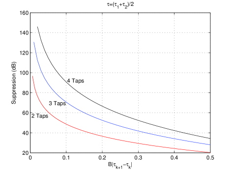
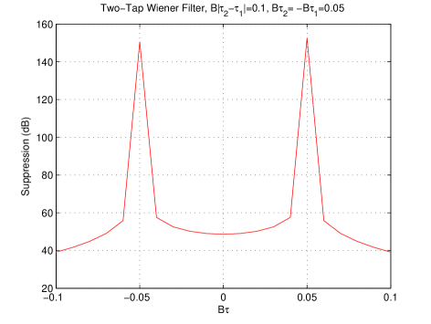
Figure 1: Performance of Wiener filter: (a) Effect of normalized tap delay difference and number of taps (b) Effect of echo delay location in two tap Wiener filter with normalized tap delay difference equal to 0.1.

II Echo Cancellation in Analogue Domain

Echo cancellation is a well-known topic studied extensively in the literature and proved technology in the field. Despite the comprehensive investigations, the derivation of algorithms and implementations are performed in digital baseband. However, as described previously in Section I, the echoes should be cancelled before LNA i.e. in analogue domain. Implementing digital signal processing techniques in analogue domain is very challenging due to RF impairments and the fact that only limited mathematical operations are allowed in analogue domain. In this section, we derive echo cancellation techniques in analogue domain and show that our method can cancel echoes very effectively even with RF impairments.

II-A System Model and Wiener Solution in Analogue

The transmitted signal in passband can be written as

$$x(t) =Re\{\left(x_{i}(t)+jx_{q}(t)\right)e^{-j\omega t}\}$$ (1)

$$=x_{i}(t)\cos(\omega t)+x_{q}(t)\sin(\omega t)$$ (2)

where $Re\{\cdot\}$ represents the real part, $\omega$ is the carrier frequency in radian/sec, and $x_{i}(t)$ and $x_{q}(t)$ are baseband in-phase and quadrature phase signals, respectively. Without loss of generality, we assume one echo with unknown gain and delay. Then, the received signal $y(t)$ at receive chain can be modeled as

$$y(t)=gx(t-\tau)+r(t)+n(t)$$ (3)

where $g$ and $\tau$ are the unknown gain and delay of the echo, respectively, $r(t)$ is the desired received signal and $n(t)$ is additive white Gaussian noise (AWGN). In this paper we cancel the echo in passband by creating estimated echo signal using multiple replica of $x(t)$ with different delays and subtracting it from the signal corrupted by echo. For instance, the echo can be estimated by a linear combination of $x(t-\tau_{1})$ and $x(t-\tau_{2})$ where $\tau_{k}$ is the delay of $k$-th tap. In order to rotate the phases of $x(t-\tau_{1})$ and $x(t-\tau_{2})$, we also need to use the Hilbert transform of $x(t-\tau_{1})$ and $x(t-\tau_{2})$. Then, the estimated echo using two taps can be written as

$$e(t)=w_{1i}x(t-\tau_{1})+w_{1q}\hat{x}(t-\tau_{1})+w_{2i}x(t-\tau_{2})+w_{2q}\hat{x}(t-\tau_{2})$$ (4)

where $w_{ki}$ and $w_{kq}$ are in-phase and quadrature component of $k$-th tap weight, and $\hat{x}(t)=x_{i}(t)\sin(\omega t)-x_{q}(t)\cos(\omega t)$ is the Hilbert transform of $x(t)$. Then, the echo canceller output can be expressed as

$$z(t)=y(t)-e(t).$$ (5)

In order to simplify derivation of the weights $w_{ki}$ and $w_{kq}$, we transform the passband model to equivalent complex baseband model. The transmitted complex baseband signal $X(t)$ is defined by

$$X(t)=x_{i}(t)+jx_{q}(t).$$ (6)

Then, from (3), the received signal in complex baseband is in the form of

$$Y(t)=gX(t-\tau)e^{j\omega\tau}+R(t)+N(t)$$ (7)

where $R(t)$ and $N(t)$ are complex baseband versions of desired received signal and AWGN, respectively. Likewise, we can develop the complex baseband model of the echo canceller output from (4) and (5) as follows

$$Z(t)=Y(t)-W_{1}X(t-\tau_{1})e^{j\omega\tau_{1}}-W_{2}X(t-\tau_{2})e^{j\omega\tau_{2}}.$$ (8)

After some manipulations, it is not difficult to show that $W_{k}=w_{ki}+jw_{kq}$. For the concise representation, the echo canceller output can be written in vector form as

$$Z(t)=Y(t)-\textbf{{W}}^{T}\textbf{{X}}(t)$$ (9)

where superscript $(\cdot)^{T}$ represents transpose, $\textbf{{W}}=[W_{1}~{}W_{2}]^{T}$ and $\textbf{{X}}(t)=[X(t-\tau_{1})e^{j\omega\tau_{1}}~{}X(t-\tau_{2})e^{j\omega\tau_{2}}]^{T}$.

Although it is not possible to implement Wiener solution in analogue domain, minimum mean squared error (MMSE) solution provides valuable insights on the performance and design parameters. Minimizing the power of the echo canceller output means that the echo is cancelled. This is due to the fact that unknown desired receive signal $r(t)$ and AWGN cannot be cancelled by linear combination of $\{x(t-\tau_{k})\}$ as $\{x(t-\tau_{k})\}$ is uncorrelated with $r(t)$ and noise. Therefore, we define the cost function which minimizes the power of the echo canceller output as

$$\min_{\textbf{{W}}}E\{|Z(t)|^{2}\}=\min_{\textbf{{W}}}E\{|Y(t)-\textbf{{W}}^{T}\textbf{{X}}(t)|^{2}\}.$$ (10)

In Appendix A the derivation of Wiener solution in analogue domain is presented. Echo cancellation performance is shown in Fig. 1 where the suppression level is defined by

Suppression $$=\frac{\text{Echo Power}}{\text{Residual Echo Power}}$$ (11)

$$=\frac{E\{|gX(t-\tau)|^{2}\}}{E\{|gX(t-\tau)e^{j\omega\tau}-\textbf{{W}}^{T}\textbf{{X}}(t)|^{2}\}}.$$ (12)

The suppression is not a function of the carrier frequency and echo power as shown in Appendix A. Rather, it is a function of delay difference between taps and the number of them. Fig. 1 (a) exhibits suppression as a function of tap delay difference normalized by signal bandwidth (B) assuming that the echo delay is in the middle of the first and second tap delay. As it can be observed from the figure, smaller normalized tap delay difference $\left(B|\tau_{2}-\tau_{1}|\right)$ and larger number of taps provide better echo suppression. Even with two taps, the suppression level close to 90 dB can be achieved with the normalized tap delay difference equal to 0.01 which means 1 nsec of delay difference between taps in 10 MHz bandwidth systems. This is equivalent to 100 times oversampling in digital signal processing. It is apparent that as the tap delay difference goes to zero the suppression level goes to infinity (i.e. no residual echo). We emphasize that having a small tap delay difference is not a challenging issue. For example, assuming the speed of electromagnetic (EM) wave in transmission line is equal to the speed of light, $3mm$ difference in length will yield $10$ pico second delay difference. In Fig. 1 (b) the effect of echo delay on echo canceller performance is illustrated assuming that the normalized tap delay difference is 0.1. In reality the delay of echo is unknown. However, typical value or range of values of circulator delay can be measured. Interestingly, when the tap delay coincides with the true delay of the echo, even with only two taps suppression beyond 150 dB can be easily achieved. The reason that even when $\tau$ is equal to either $\tau_{1}$ or $\tau_{2}$ the suppression is not infinity is that $\tau_{2}-\tau_{1}$ is not approaching zero. It is simple to show that when the delay of either taps coincides with the echo delay, one tap echo canceller instead of two tap echo canceller has infinity suppression level.

In two tap Wiener filter, we study the impact of number of echoes under the condition of same total echo powers. Assume one echo having delay $\tau$ located in the middle of neighboring two taps

$$Y_{1}(t)=X(t-\tau)e^{j\omega\tau}$$ (13)

where $\tau=(\tau_{1}+\tau_{2})/2$. Without loss of generality assume $E\{|X(t)|^{2}\}=1$. Let us add one more echo with the same power as the first echo but closer to the second tap with arbitrary phase $\vartheta$ and delay $\tau+\delta$ where $0<\delta<(\tau_{2}-\tau_{1})/2$ and $\tau_{2}>\tau_{1}$. Then, the received echo signal becomes

$$Y_{2}(t)=X(t-\tau)e^{j\omega\tau}+X(t-\tau-\delta)e^{j\omega(\tau+\delta)+\vartheta}.$$ (14)

The power of $Y_{2}(t)$ is

$$E\{|Y_{2}(t)|^{2}\}=2\left(1+\cos(\omega\delta+\vartheta)Sinc(B\delta)\right).$$ (15)

Depending on the phase $\omega\delta+\vartheta$, the new echo can reduce total echo power. However, we consider the worst case i.e. $\cos(\omega\delta+\vartheta)=1$. Note $Sinc(B\delta)>0$ due to the assumption $B\delta<1$. For fair comparison, we normalize $Y_{2}(t)$ such that maximum power of $Y_{2}(t)$ is equal to the power of $Y_{1}(t)$

$$Y_{2}(t)=c\left(X(t-\tau)e^{j\omega\tau}+X(t-\tau-\delta)e^{j\omega\tau}\right)$$ (16)

where $c=1/\sqrt{2+2Sinc(B\delta)}$. Then, $Y_{1}(t)$ and $Y_{2}(t)$ have the same power but $Y_{1}(t)$ has one echo in the middle of taps while $Y_{2}(t)$ contains two echoes: one in the middle of the taps and the other closer to either taps.

The cross correlation vector can be written as

$$\textbf{{R}}_{Y_{2}\textbf{{X}}}=E\{Y_{2}(t)\textbf{{X}}^{H}(t)\}=ce^{j\omega\tau}(\textbf{{r}}_{{}_{Y\textbf{{X}}}}+\textbf{{r}}_{{}_{Y_{2}\textbf{{X}}}})\textbf{{D}}$$ (17)

where $\textbf{{r}}_{{}_{Y\textbf{{X}}}}$ and D are defined in Appendix A and

$$\textbf{{r}}_{{}_{Y_{2}\textbf{{X}}}}=[Sinc(B(\tau+\delta-\tau_{1}))~{}Sinc(B(\tau+\delta-\tau_{2}))].$$ (18)

It is not difficult to show the residual echo powers of $Y_{1}(t)$ and $Y_{2}(t)$ as following

$$mse_{1} {}={} 1-\textbf{{r}}_{{}_{Y\textbf{{X}}}}\textbf{{r}}_{{}_{\textbf{{XX}}}}^{-1}\textbf{{r}}_{{}_{Y\textbf{{X}}}}^{H}$$ (19)

and,

$$mse_{2}=\frac{mse_{1}+mse_{0}+2(Sinc(B\delta)-\textbf{{r}}_{{}_{Y_{2}\textbf{{X}}}}\textbf{{r}}_{{}_{\textbf{{XX}}}}^{-1}\textbf{{r}}_{{}_{Y\textbf{{X}}}}^{H})}{2+2Sinc(B\delta)},$$ (20)

respectively where $mse_{0}=1-\textbf{{r}}_{{}_{Y_{2}\textbf{{X}}}}\textbf{{r}}_{{}_{\textbf{{XX}}}}^{-1}\textbf{{r}}_{{}_{Y_{2}\textbf{{X}}}}^{H}$ which is the residual echo power of the second echo when the first echo is not present.

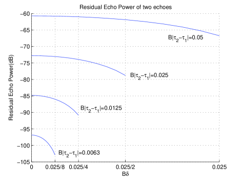
Figure 2: Effect of two echoes in two tap Wiener filter.

From Fig. 2 it is clear that as the second echo moves toward the second tap, the residual echo power is reduced. Notice that $\delta=0$ means that only one echo exists. Hence, the assumption of one echo in the middle of neighboring taps is the worst simulation condition. This is from the fact that echo closer to either tap is easier to estimate as shown in Fig. 1 (b). The argument can be easily extended to arbitrary number of echoes with arbitrary echo powers located between neighboring taps.

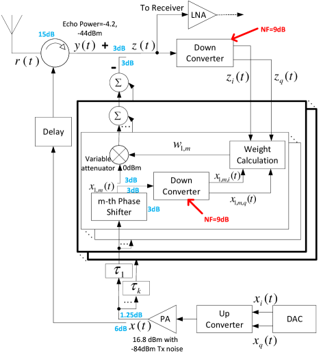
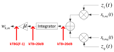
Figure 3: Block diagram of adaptive echo cancellation in analogue domain: (a) High level block diagram (b) Weight calculation block.

II-B Adaptive Echo Cancellation in Analogue

In the previous subsection ideal phase shifter is assumed for Hilbert transform. However, due to phase imbalance in phase shifter, Hilbert transform of $x(t-\tau_{k})$ will not be orthogonal to $x(t-\tau_{k})$. To overcome the phase imbalance problem we use multiple phase shifters. As far as those phases are not identical, by a linear combination of the multiple phase shifter outputs we can rotate and scale $x(t-\tau_{k})$ even with large phase imbalances. Assuming $K$ taps and $M$ phase shifters per tap, $m$-th phase shifter output at $k$-th tap can be written as

$$x_{k,m}(t)=g_{k,m}\{ x_{i}(t-\tau_{k})\cos(\omega(t-\tau_{k})-\theta_{k,m})$$

$$+ x_{q}(t-\tau_{k})\sin(\omega(t-\tau_{k})-\theta_{k,m})\}$$ (21)

where $g_{k,m}$ is phase shifter gain to represent amplitude imbalance, and $\theta_{k,m}$, which can be modeled as $\pi m/M+\phi_{k,m}$, is phase shift including phase imbalance $\phi_{k,m}$. It is clear that with $M=3$, as far as the phase imbalance is less than $30^{\circ}$, those three phases will not be identical. By a linear combination of phase shifter outputs, echo can be estimated as follows

$$e(t)=\sum_{k=1}^{K}\sum_{m=1}^{M}w_{k,m}x_{k,m}(t)$$ (22)

where $w_{k,m}$ is real valued weight for $k$-th tap and $m$-th phase shifter. The complex baseband model of echo canceller output $z(t)$ can be developed from (5) and (22) as

$$Z(t)=Y(t)-\sum_{k=1}^{K}\sum_{m=1}^{M}w_{k,m}X_{k,m}(t).$$ (23)

where $X_{k,m}(t)$ is complex baseband version of $x_{k,m}(t)$. The real and imaginary parts of $X_{k,m}(t)$ can be written as

$$X_{k,m,i}(t)=g_{k,m}\{ x_{i}(t-\tau_{k})\cos(\omega\tau_{k}+\theta_{k,m})$$

$$- x_{q}(t-\tau_{k})\sin(\omega\tau_{k}+\theta_{k,m})\},$$ (24)

and

$$X_{k,m,q}(t)=g_{k,m}\{ x_{i}(t-\tau_{k})\sin(\omega\tau_{k}+\theta_{k,m})$$

$$+ x_{q}(t-\tau_{k})\cos(\omega\tau_{k}+\theta_{k,m})\},$$ (25)

respectively. Since implementing Wiener filter in analogue domain is quite difficult if not impossible, it is desirable to design techniques which are implementable in analogue domain. For this end, we apply well-known steepest-descent method to the cost function (10). This leads to

$$w_{k,m} =w_{k,m}-\frac{\mu}{2}\frac{\partial|Z(t)|^{2}}{\partial w_{k,m}}$$

$$=w_{k,m}+\mu Re\{X_{k,m}^{*}(t)Z(t)\}$$ (26)

where $\mu$ is step-size and superscript $(\cdot)^{*}$ represents complex conjugate. Notice that cross correlation $Re\{X_{k,m}^{*}(t)Z(t)\}$ can be served as echo channel estimation at $k$-th tap delay of $m$-th phase shifter output. Since it is quite noisy estimation due to random signal $x(t)$, noise and impairments which will be discussed in next subsection, the noisy estimation is low-pass filtered by integrator with small step-size $\mu$ as shown in (26).

Together with (26), (5) leads to the block diagram of the adaptive echo cancellation in analogue domain shown in Fig. 3. Note that the multipliers in the outputs of phase shifters are in fact variable attenuators since the magnitudes of weights can be limited to less than 1 by design. Also notice that as the step-size $\mu$ is much less than 1, it can be implemented by a fixed attenuator. Overall, it is quite clear that the proposed structure is implementable.

II-C Impairments

Unfortunately, however, $\{X_{k,m}(t)\}$ and $Z(t)$ cannot be obtained due to phase noise, phase/amplitude imbalances in downconverter. With unknown phase error $\phi_{z,i}$ and $\phi_{z,q}$ in in-phase and quadrature phase respectively, and unknown gains of $g_{z,i}$ and $g_{z,q}$ in in-phase and quadrature phase respectively, following signal has to be used

$$\widetilde{Z}(t)=g_{z,i} Re\{Z(t)e^{-j(\phi_{z,i}+\varphi_{z}(t))}\}$$

$$+jg_{z,q} Im\{Z(t)e^{-j(\phi_{z,q}+\varphi_{z}(t))}\}$$ (27)

where $Im\{\cdot\}$ represents imaginary part and $\varphi_{z}(t)$ is phase noise. Similarly, we can define $\widetilde{X}_{k,m}(t)$. In addition, although all downconverters are driven by the same oscillator, each downconverter may have different phase rotation. Hence, effectively following will be performed

$$w_{k,m} =w_{k,m}+\mu Re\{\widetilde{X}_{k,m}^{*}(t)\widetilde{Z}(t)e^{j\Delta_{k,m}}\}$$ (28)

where $\Delta_{k,m}$ is the phase difference between downconverter for $Z(t)$ and downconverter for $X_{k,m}(t)$. It is desirable to have $\Delta_{k,m}<45^{\circ}$ in order to avoid divergence or slow convergence. Next, the effect of phase distortion in the variable attenuator is investigated. In wideband variable attenuator [12], different attenuation causes different phase rotation $e^{j\phi(w_{k,m})}$. Thus the second term in the right-hand side of (28) is changed to

$$\mu Re\left\{\widetilde{X}_{k,m}^{*}(t)\widetilde{Z}(t)e^{j(\Delta_{k,m}-\phi(w_{k,m}))}\left(1-jw_{k,m}\frac{\phi(w_{k,m})}{\partial w_{k,m}}\right)\right\}.$$ (29)

As in [12], the phase distortion can be modeled as a linear function of attenuation in log scale. For example, assuming $0^{\circ}$ and $50^{\circ}$ phase rotations at 3 dB and 38 dB attenuations respectively leads to

$$w_{k,m} =w_{k,m}+\mu Re\left\{\widetilde{X}_{k,m}^{*}(t)\widetilde{Z}(t)e^{j\left(\Delta_{k,m}-\phi(w_{k,m})+12^{\circ}\right)}\right\}.$$ (30)

The additional phase rotation due to the phase distortion in the attenuator can be absorbed in $\Delta_{k,m}$. The phase distortion is large when the attenuation is large. However, when the attenuation is large, its contribution to echo estimation is small. Thus, the phase distortion at high attenuation can be ignored. The values of above mentioned impairments are unknown. Hence, we do not take any attempt to compensate those impairments in our study. Simply, the outputs of downconverters which include all those impairments are used to train the weights.

Although the second terms in the right hand side of (26) and (30) are quite different due to impairments, as far as the signs of the second terms are same, the adaptive technique can converge as explained in Appendix B. This is why the proposed method exhibits immunity to impairments unlike open loop techniques.

The fixed phase shifter, combiner, splitter and coupler are quite linear components. In [12], the input third order intercept point (IIP3) of the variable attenuator is 50 dBm which means with 0 dBm input power non-linear distortion power can be less than -100 dBm. Hence, 0 dBm input power at the variable attenuator is maintained.

TABLE I: Phase/Amplitude imbalances : In the order of Phase shifter/Downconverter I/Q

	Phase Imbalances & $\Delta_{k,m}$			Amplitude Imbalances
$k$	$\phi_{k,m}$, $\phi_{x,k,m,i}$, $\phi_{x,k,m,q}$, $\Delta_{k,m}$			$g_{k,m}$, $g_{x,k,m,i}$, $g_{x,k,m,q}$
	$m=1$	$m=2$	$m=3$	$m=1$	$m=2$	$m=3$
Tap 1	-1, 0.6, 0.3, 30∘	10, 0.1, 1.1, -30∘	5, 0.25, -0.75, 15∘	-0.5, 0.2, 0.7 dB	1, 0.1, 0.6 dB	1, 0.23, -0.27 dB
Tap 2	11, -0.5, 0.5, 10∘	-2, 0.5, -0.4, 23∘	2, -0.15, 0.8, -17∘	-1, -0.1, 0.4 dB	0.5, 0.5, -0.1 dB	2, 1, 0.5 dB
Tap 3	2, -0.8, 0.2, -25∘	12, -0.2, 0.8, 19∘	-5, 0.7, -0.2, -30∘	1.5, -0.3, 0.2 dB	-0.2, -0.2, 0.3 dB	2, 0.4, -0.1 dB

At the output of every component, noise with power of $kTBG(F-1)$ is added where $kTB$ represents thermal noise power over bandwidth $B$, $G$ is power gain and $F$ is noise factor. In passive components including the variable attenuator $F=1/G$ is assumed. The loss of power in component is specified in Fig. 3. $N$-way combiner and splitter are assumed to have loss of $10\log_{10}N$ per branch (not shown in Fig. 3). The noise figure of downconverter is assumed to be 9 dB. As shown in Fig. 3 (b), 20 dB of noise above thermal noise is added at the integrator output. For the noise in baseband multipliers and adder we equivalently add 20 dB of noise above thermal noise.

BS and AP may not need to support multiple bands in a given operator and deployment. However, terminal will need to support multiple bands. Multiband support is more pronounced in cellular systems. It is more challenging to have good antenna match over multiple bands in terminal. Hence, dominant echo can come from antenna mismatching in terminals. Considering terminal, we assume echo power of only 15 dB lower than transmit power mainly due to antenna mismatching although typical broadband commercial circulator has isolation of 20 $\sim$ 25 dB with fractional dB of insertion loss. Notice that BS and AP can accommodate bulky circulator which can provide more than 40 dB isolation and will need to tune antenna for fewer number of bands usually. By better antenna match and smaller leakage in circulator, the 6 and 3 dB loss of signal power in couplers in transmit and receive path respectively can be reduced by increasing the loss of coupler in echo estimation path.

Table I shows phase imbalances in phase shifters ($\phi_{k,m}$) and corresponding downconverters’ in-phase and quadrature phase imbalances($\phi_{x,k,m,i},\phi_{x,k,m,q}$) relative to in-phase of transmit signal. The phase rotation difference $\Delta_{k,m}$ is specified as well. Amplitude imbalances in phase shifters ($g_{k,m}$) and corresponding downconverters’ in-phase and quadrature phase amplitude imbalances ($g_{x,k,m,i},g_{x,k,m,q}$) relative to in-phase of transmit signal are tabulated in Table I. In the downconverter for $z(t)$, phase imbalances of $-0.9^{\circ}$ and $0.1^{\circ}$, and amplitude imbalances of -0.1 dB and 0.4 dB are assumed for in-phase and quadrature phase, respectively. In transmit chain, it is assumed that the quadrature phase has $1.5^{\circ}$ phase and 0.8 dB amplitude imbalance relative to in-phase. Note that phase and amplitude imbalances larger than commercially available components are assumed. Regarding DC-offset, zero DC-offset is considered which can be achieved by DC blocking capacitor.

From the derivation of adaptive echo cancellation, no restriction on transmitted signal is imposed. Hence, even if transmitted signal $x(t)$ is contaminated by impairments such as phase/amplitude imbalance, non-linear distortion, phase noise, and additional noise above thermal noise, the performance in analogue domain is unaffected as long as the bandwidth is remained the same. Of course, when the signal bandwidth is changed due to impairments, the tap delay difference $|\tau_{k+1}-\tau_{k}|$ should be adjusted accordingly to maintain the same normalized tap delay difference. In adaptive echo cancellation and Wiener filter, the echo $x(t-\tau)$ is estimated by linear combination of $\{x(t-\tau_{k})\}$. Thus, it is important for the input signal to echo estimation path to be identical to the input signal to echo channel path. However, in digital domain echo cancellation, this property cannot be met. This is a significant advantage over digital domain echo cancellation where the digital baseband signal which goes to echo estimation path does not contain all RF impairments in transmit chain.

II-D Simulations

Instead of training sequence, 10 MHz random OFDM signals with 102 active subcarriers and QPSK symbols are transmitted. A white noise 20 dB above thermal noise is added to OFDM signal right after power amplifier as a transmit noise. At the output of circulator two echoes are created in simulations and an echo canceller with three taps is considered. The first echo with -4.2 dBm power is located in the middle of the first and second tap delay, and the second echo with -44 dBm power is located in the middle of the second and third tap delay. We set the normalized tap delay difference $B|\tau_{k+1}-\tau_{k}|$ to be 0.025 which is equivalent of 40 times oversampling in delay domain. This means that the delay spread is 2.5 nsec. Note that with three taps we can cancel echoes of 5 nsec delay spread at least.

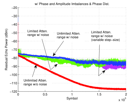
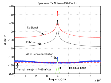
Figure 4: Adaptive analogue echo canceller with 3 taps, $B|\tau_{k+1}-\tau_{k}|=0.025$ and two echoes (-4.2 and -44 dBm): (a) Convergence (b) Spectrum.

In Fig. 4 (a) simulation results of adaptive echo cancellation in analogue domain are demonstrated. Assuming 12.5% of guard interval $2\times 10^{5}$ symbols translate 2.32 sec. Aforementioned all impairments excluding phase noise are assumed. When unlimited dynamic range is assumed in the variable attenuator without noise, the in-band residual echo power is far less than thermal noise power -104 dBm. In this case, more than 110 dB of suppression which is close to Wiener filter solution is possible (see Fig. 1 (a)). When impairments do not limit the performance, the adaptive echo cancellation can converge to Wiener solution. The suppression level in Wiener filter is not a function of absolute power of echo but the number of taps and the normalized tap delay difference. The result demonstrates that the phase/amplitude imbalances and phase distortion are not limiting factors.

When RF impairments do not limit performance, it is not difficult to show that more suppression of echo can be achieved by smaller normalized tap delay difference as demonstrated in Wiener filter section. This is one of benefits in analogue domain echo cancellation since high oversampling for digital domain processing is not feasible. However, by decreasing the normalized tap delay difference, convergence becomes slower while echo cancellation performance improves. This slower convergence is typical behavior of larger eigenvalue spread of auto-correlation matrix of tap input in adaptive filter [13]. It is clear that by decreasing the normalized tap delay difference, the eigenvalue spread of the auto-correlation matrix of tap input (A.10) becomes larger.

By adding noise, however, we observe slow convergence and higher floor. When the dynamic range of the attenuator is limited to 35 dB(i.e. 3 $\sim$ 38 dB attenuation), fluctuation is noticeable since the limited dynamic range will interfere the convergence behavior especially when weights have to change signs. It is clear that as the residual echo power becomes smaller, the variance of the residual echo power increases. This is due to the fact that as the echo power is reduced, SNR from echo point of view worsens. When noise becomes effective, the variance can be reduced by smaller step-size [13]. As seen in Fig. 4 (a) the residual echo power can be less than -90 dBm when the step-size is reduced by half at $1.5\times 10^{5}$ symbol. Simple noise analysis shows that heavy noise at weight calculation block (20 dB of noise before and after integrator) governs the absolute value of residual echo power as it reduces the SNR of residual echo and directly affects the weight calculation (30). It is critical to reduce the noise at baseband and improve the dynamic range of the attenuation. Fig. 4 (b) exhibits the spectrum when the residual echo power is -90 dBm. It is interesting to note that the out-of-band power of $z(t)$ at vicinity of in-band is equal to thermal noise (=-174 dBm/Hz) even if transmit noise is -154 dBm/Hz. This demonstrates that the transmit noise above thermal noise can be cancelled as well. However, the noise power at frequencies far from in-band is a bit higher than thermal noise. Note that the cost function (10) will be driven by high power component in frequency. Hence, the weights are mainly influenced by in-band signal. Thus, as far as out-of-band power is smaller than in-band power, weights will be chosen to reduce in-band power. In addition, the normalized delay difference is not sufficiently small to cancel out-of-band noise. Therefore, less reduction of echo in out-of-band is possible. It is clear that the proposed structure is enough for duplexer free systems and device co-existence problem. However, the residual echo power is too high to operate STR unless the noise at baseband is decreased and the dynamic range in the attenuator is improved.

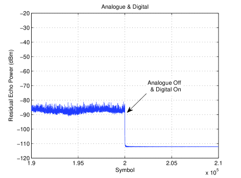
Figure 5: Analogue and digital echo cancellation.

We bring attention to the prototypes in [1], [8], [9] where additional 20 $\sim$ 30 dB of echo suppression is achieved by digital domain echo cancellation. When the power of $z(t)$ is less than a threshold, the analogue weight update is disconnected and digital domain echo cancellation is enabled. By disconnecting from analogue update circuit, the heavy noise from baseband and other impairments will not appear in receive chain via weights. Also by turning off the analogue weight calculation block and multiple downconverters, power consumption can be reduced. In this paper simple open-loop technique is applied for digital domain echo cancellation. The echo channel at every subcarrier is estimated and this estimation is averaged over time. From the estimated echo channel, echo signal is estimated at every subcarrier and subtracted from received signal. The joint simulation of analogue and digital echo cancellation is shown in Fig. 5. It is clear that the residual echo power is less than thermal noise. In fact due to large noise figure in receive chain (5 dB in BS and 9 dB in UE for example), the background noise will be -99 dBm and -95 dBm respectively. This will give us more tolerance in phase/amplitude imbalance in transmit chain.

II-E Phase noise and Time varying channel

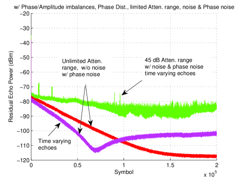
Figure 6: Convergence with white phase noise ($\sigma=2^{\circ}$) and time varying echoes.

In this subsection, phase noise is added on top of the previous simulation conditions. Phase noise is assumed to be white Gaussian noise with root mean square (rms) equal to 2 degree. All downconverters are assumed to have independent phase noises. From Fig. 6, when noise free and unlimited attenuation range in variable attenuator are assumed, the convergence behavior is almost identical to the case without phase noise (see Fig. 4 (a)). It is evident that the white phase noise is not a limiting factor. As explained in Appendix B, the phase noise effectively reduces the average power of echo channel estimation (Appendix B). This means that the SNR from residual echo point of view is smaller when noise is present. Hence, in this case noise at baseband becomes more prominent than the case without phase noise. The main reason why the proposed method is less sensitive to phase noise is that the phase noise does not directly appear at weights. Rather, the phase noise is low-pass filtered with small step-size $\mu$ which controls the bandwidth of the low pass filter. Hence, unlike open-loop techniques, the closed-loop techniques such as adaptive filter has good level of immunity to impairments. In [14] an analysis on the phase noise impact to echo suppression is reported when open-loop technique is applied. From the analysis, only 26 dB of echo suppression is possible when rms phase noise is $2^{\circ}$. Note that open-loop technique is directly sensitive to various impairments as impairments deteriorate the accuracy of echo channel estimation.

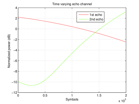
Figure 7: Time varying echo channel.

Next, we consider the effect of time varying channel. The echoes reflected from objects in time varying wireless channel and coming back to receive antenna have large path loss due to round trip. Since these objects introduce additional loss and also orientations of the objects are not always positioned toward receive antenna, in general these echoes have relatively small powers. In all other proposals which employ separate transmit and receive antenna, all echoes, including the strongest echo, come from over-the-air channel. Therefore, the strongest echo can be more time variant compared to our proposal. This is due to the fact that, in our proposal the strongest echo comes from RF components inside device which usually has good shielding and consequently, much less time variation of echo channel is expected. Nonetheless, to demonstrate the capability of tracking time varying echoes, we simulate time varying echo channels. The time varying impulse response is shown in Fig. 7. The first echo has 4.7 dB of dynamic range while the second echo has 14 dB of power change over $2\times 10^{5}$ OFDM symbols. First, let us focus on the case when unlimited attenuation range and noise free are assumed. Since the prediction of time varying channel is not possible, higher residual echo power is unavoidable. In addition, the second echo power is growing. Thus, when the residual power of the second echo becomes more dominant than that of the first echo, the residual echo power is increased as well since the supersession level is fixed regardless of absolute power of echo. For faster tracking the step-size is increased in this simulation.

As addressed earlier limited range of attenuation interferes smooth change of sign of weights. Hence, glitches in convergence are observed as seen in Fig. 4 (a). Although adaptive algorithm quickly stabilizes the convergence owing to negative feedback, for smoother tracking of time varying channel it is desirable to increase the attenuation range. Therefore, we assumed 45 dB range of attenuation. As seen in Fig. 6, even in this severe time varying channel, our proposed technique converges very well. In general, adaptive filter has good level of capability in tracking time varying channel owing to closed-loop operation. In open-loop technique, the echo cancellation performance is directly coupled with echo channel estimation error. For better echo cancellation, more accurate channel estimation is required and consequently, we will need to average the impulse response for longer period of time. This means that the capability of tracking time varying channel is fundamentally limited. However, in closed-loop technique, when the residual echo signal $Z(t)=Y(t)-E(t)$ becomes suddenly large due to any reason, the power of second term in right hand side of (26) which drives the weights is increased as well. Therefore, the weights are immediately changed to reduce the power $|Z(t)|^{2}$.

II-F Discussions

Although in the simulations two echoes are assumed, multiple echoes with same delay can be treated as one echo. In reality the delay spread of echoes should be measured, and first and second tap delays should be decided in order to cover the delay spread. If the tap delay difference is too large, more taps are needed between these two taps in order to make sure the normalized tap delay difference between neighboring taps $B|\tau_{k+1}-\tau_{k}|$ to be sufficiently small. For any pair of neighboring taps, we added only one echo with delay equal to the middle of two neighboring taps. As demonstrated earlier, this is the worst case scenario. The residual echo power is less dependent on the number of echoes but more on the total echo power and normalized delay difference $B|\tau-\tau_{k}|$ where $\tau$ is echo delay and $\tau_{k}$ is the delay of nearest tap. In order to have sufficient degrees of freedom, the number of taps should be large enough to cover the delay spread and minimize normalized delay difference $B|\tau-\tau_{k}|$.

We emphasize that RF implementations for adaptive duplexers or duplexer free systems [4], [15] are similar to our proposed structure except weight calculation algorithm as those use the same building blocks such as phase shifters and variable attenuators in passband. In addition, echoes appear at receive chain via either circulator or duplexer. However, those prototypes make a null at a particular frequency, which means that the algorithm does not take care of other frequencies. Thus, it cannot create wide null and out-of-band power can be large. In contrast, our scheme chooses weights which minimize the power of echo canceller output over whole band. Hence, out-of-band residual echo power is not higher than in-band residual echo power. Of course, by filtering $z(t)$ weights can be optimized for a particular band. It is interesting to note RFIC product [16], [17] in which adaptive blind receive beamforming is implemented in analogue domain. From [17] it is evident that weights are adaptively calculated in analogue baseband and applied in passband to achieve receive beamforming in RF. The high level structure which implements adaptive algorithm in [17] is similar to our proposal although the objective and detail algorithms are different.

From simulation results within 20 $\sim$ 30 symbols (0.23 $\sim$ 0.35 msec) the residual echo powers reach -70 $\sim$ -77 dBm. Note that the weights are initialized to lowest positive values which are irrelevant to echo channel impulse response. However, the weights are quickly trained to reduce the residual echo power to -70 $\sim$ -77 dBm. For extra 10 $\sim$ 20 dB suppression, 1 $\sim$ 2 $\times 10^{5}$ symbols are needed. For faster convergence, variable step-size can be applied. Initially, the algorithm can start with large step-size (meaning large bandwidth of low pass filter) for faster initial convergence and later the step-size can be reduced for refinement and reducing noise impact. By well-designed training sequence, fast convergence and small variation of residual echo power can be obtained as well. Adaptation of weights can be done in initial start-up of the device or during production. Moreover, lower power training sequence can be used to update the weights before entering network. Note that unlike echo channel in an echo canceller that employs separate transmit and receive antennas, echo channel at circulator can vary over time with much slower rates. Therefore, it is sufficient to calculate weights in the initial power up. In order to compensate any possible drift of circulator channel, it is adequate to update the weights during preamble or for a short period during which no reception of signal is expected or the received power is small. Since updating weights does not have to be performed always, additional power consumption due to multiple downconverters and weight calculation blocks can be insignificant.

We demonstrated the feasibility of the echo canceller implementation in analogue domain with RF impairments. Given degrees of freedom such as number of taps and tap delay difference, the adaptive technique searches best weights such that echo power is minimized over entire band. Impairments will interfere convergence and may increase residual echo power. However, the negative feedback mechanism provides a certain extent of immunity to impairments. When baseband noise is high and dynamic range of variable attenuator is limited, digital baseband echo cancellation can be accompanied. It is also clear that the proposed technique can be easily extended to any MIMO system. However, one should note that in that case the echo cancellation complexity will be exponentially increased due to the cross talks coming from adjacent transmit antennas. Nonetheless, applying analogue echo cancellation to MIMO systems is not impossible. It is apparent from the formulations that the echo does not have to be the same type of radio signal as received signal. For example $r(t)$ can be WLAN signal while $x(t)$ can be Bluetooth signal.

III MAC Level Simulations in CSMA Networks

In this section the benefits of STR in CSMA networks are studied. We explore both single cell and multiple cells in order to study the effect of STR in reducing the hidden node issue and improving throughput. It is assumed that any node has the same coverage radius $r$ and signal is not reached beyond the radius. Hence, any two nodes within a distance of $r$ can sense each other’s channel activity. The hidden node problem is the major source of collisions. In a cell, downlink signal can be detected over entire cell coverage. Therefore, during downlink no collision will happen. However, in uplink when one terminal is located at cell edge while other terminal is located at the cell edge in the opposite side of the cell, these two terminals are hidden from each other. Thus, the packets from these two nodes can collide with each other. It is hard to eliminate the hidden node issue in CSMA networks due to the nature of channel sensing mechanism. However, it is clear that STR can reduce the hidden node issue. In fact, in a single cell the hidden node problem can be completely resolved by employing STR and sending a dummy packet. More precisely, as illustrated in Fig. 8 (a), whenever an AP or terminal receives a designated packet (A), if it sends a dummy packet (A$\sim$), hidden nodes can sense the channel as busy and therefore they will hold packets. We refer to this technique as s-STR.

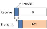
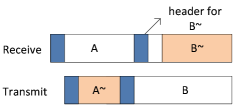
Figure 8: Frame (a) s-STR: send a dummy packet(A$\sim$) upon successful reception of the header (b) i-STR: example of collision (c) d-STR: asynchronous arrival of transmit and receive packets.

Unfortunately, there is another source of collision. In real world systems, it takes some time for any node to detect energy, or decode a header and make a decision on channel activity. In other words, it is not instant to decide whether the channel is busy or idle. Let $h$ be the elapsed time for detecting the energy of received signal or decoding a header represented in percentage of packet duration. When $h$ is non-zero, some collisions occur that are unavoidable even by means of STR. Of course in a single cell scenario with STR capability and only one active terminal, no collision occurs even with non-zero $h$. However, in general the collisions due to non-zero $h$ overshadows the gain of STR.

In order to further improve collision avoidance, we introduce i-STR which utilizes the dummy packet as an implicit ACK. Unlike traditional ACK, the implicit ACK is very immediate with the delay of only $h$ while traditional ACK has the delay of at least one packet duration. We can devise a protocol based on receiving the implicit ACK or not. For example, a destination node receiving a packet will send a dummy packet (i.e. implicit ACK) only during the period of the arriving packet if the destination successfully decodes the header of the packet. If the source node can detect the header of the implicit ACK from the destination node, it continues its current transmission. Otherwise, it stops the current transmission. Likewise, when the destination node cannot decode the header, it will not transmit the implicit ACK. Then, the source node stops the transmission. This modification will release the channel much earlier than simply sending the packet and corresponding dummy packet over the whole duration of the packet. As a result, other potential nodes can access the channel. After successful reception of the header at the destination node, as in s-STR, a dummy packet is sent by the destination node. Fig. 8 (b) shows an example of i-STR when the header of dummy packet was collided at source node. Then, the source cannot detect the header of the implicit ACK. It decides no ACK transmission from the destination at time $2h$. The source stops packet transmission at time $2h$. Then, the destination node stops dummy packet transmission as well. By this fast interaction and stopping transmission when collision is detected, instead of wasting the channel, other potential nodes can utilize it.

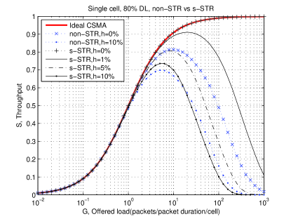
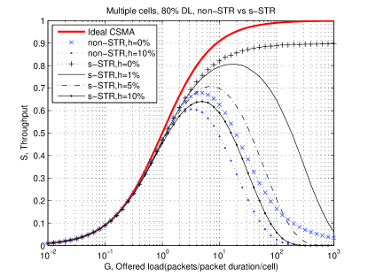
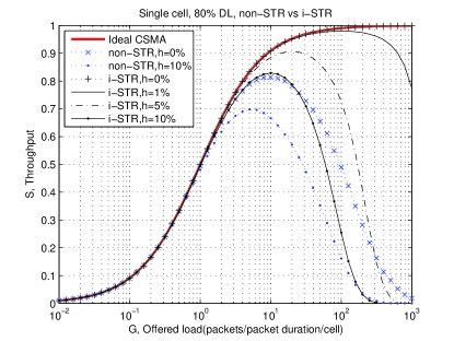
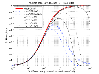
Figure 9: Throughput comparisons, DL traffic=80%: (a) s-STR in single cell (b) s-STR in multiple cells (c) i-STR in single cell (d) i-STR in multiple cells.

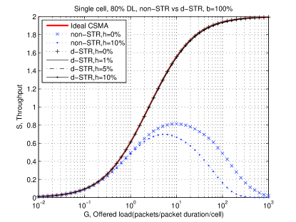
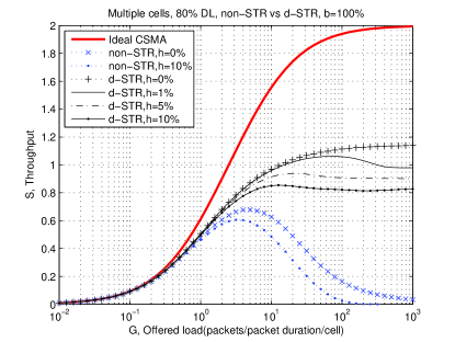
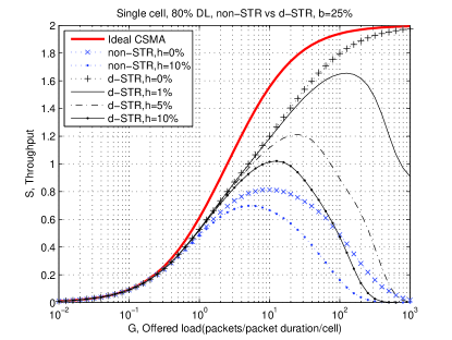
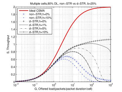
Figure 10: Throughput comparisons in d-STR, DL traffic=80%: (a) single cell, $b=100\%$ (b) multiple cells, $b=100\%$ (c) single cell, $b=25\%$ (d) multiple cells, $b=25\%$.

Simulation results for a single hop network with non-slotted transmissions, and nonpersistent CSMA [18] are presented in Fig. 9. Propagation delay is assumed to be zero in order to isolate hidden node problem from throughput degradation due to increased contention as a result of propagation delay. Terminals are assumed to be evenly and randomly distributed over the entire coverage area and operate in an infrastructure mode communicating through a central node (AP). Each packet is of constant length and packet arrival follows Poisson process. In practice, a collision does not necessarily result in packet error thanks to the near-far effect and advanced receiver. However, in our simulations we treat all collisions as packet errors. We show throughput S as a function of offered load G assuming that downlink traffic is 80% which is favorable to non-STR systems. In the figures the throughput of ideal CSMA (with no hidden node) is illustrated and can be considered as an upper bound. The throughput expression for ideal CSMA is known as

$$S=\frac{G}{1+G}.$$ (31)

Note that S is the average number of transmitted packets without collision per transmission time and G includes not only newly arrived packets but also packets waiting for retransmissions.

For multiple cell scenario we consider a 7-cell non-overlapping lay-out with one central cell and 6 cells surrounding the central cell. The data is collected from the center cell. The distance between cell centers is $2r$. In this scenario when downlink and uplink are synchronized over all cells, no collision occurs between cells. However, perfect synchronization is impossible in random access. In general, presence of neighboring cells increases the collisions and causes exposed node problem. As a result, throughput drop is unavoidable.

TABLE II: Improvement of maximum throughput over non-STR : Downlink traffic = 80%

$h$	Single cell				Multiple cells
	s-STR	i-STR	d-STR	d-STR	s-STR	i-STR	d-STR	d-STR
			(b=25%)	(b=100%)			(b=25%)	(b=100%)
0%	22.8%	22.8%	143%	145%	32.1%	47.2%	66.6%	67.9%
1%	14.0%	22.6%	107%	149%	20.4%	45.3%	52.8%	58.6%
5%	7.9%	21.2%	62.2%	166%	10.7%	37.3%	40.9%	46.6%
10%	5.4%	18.8%	46.2%	185%	5.7%	29.6%	33.2%	41.1%

TABLE III: Improvement of maximum throughput over non-STR : Downlink traffic = 50%

$h$	Single cell				Multiple cells
	s-STR	i-STR	d-STR	d-STR	s-STR	i-STR	d-STR	d-STR
			(b=25%)	(b=100%)			(b=25%)	(b=100%)
0%	63.2%	63.2%	224%	226%	76.0%	89.2%	115%	116%
1%	43.0%	60.0%	188%	231%	49.1%	83.9%	95.5%	101%
5%	27.2%	49.6%	119%	253%	26.9%	64.2%	73.1%	81.4%
10%	19.0%	39.2%	84.6%	279%	16.3%	46.7%	56.1%	67.4%

When $h=0\%$, collisions come from only hidden nodes. However, s-STR and i-STR systems do not have any collision thanks to the dummy packet and, as it can be seen in Fig. 9 (a) and (c), the corresponding throughput curves match ideal CSMA. In contrast, non-STR system suffers from hidden nodes even with $h=0\%$. This is clear evidence that the dummy packet in s-STR and i-STR systems completely resolves the hidden node issue. Apparently, i-STR outperforms s-STR in both single cell and multiple cells since i-STR releases the channel earlier when a collision is detected. In multiple cells additional loss is observed. The loss is more significant in non-STR systems. In fact in multiple cell case, the dummy packet from terminal can create collision to neighboring downlink signal. However, the gains from s-STR and i-STR in all other cases are more dominant.

Now we further modify i-STR as follows. Instead of sending a dummy packet, the destination node transmits a packet which contains information. It is apparent that the throughput will be doubled whenever the destination node sends a packet while it receives a packet. However, due to random packet arrival, it is not always a realistic assumption that the arrivals of transmit and receive packet are synchronized. To be realistic we again assume Poisson distribution for packet arrival. In this asynchronous transmission, new packet B as shown in Fig. 8 (c) will overwrite the dummy packet A$\sim$. The header for the implicit ACK for new packet B can be embedded or interleaved in the packet A. This technique will be referred to as d-STR. In d-STR, the ideal throughput is obtained as follows

$$S=\frac{pG}{1+pG}+\frac{(1-p)G}{1+(1-p)G}$$ (32)

where $p$ represents the probability of downlink packet. Notice that as $G$ goes to infinity, the throughput $S$ converges to 2 when $p\neq 1$ and $p\neq 0$. Since asynchronous transmit and receive packet generation is assumed, we define following probability

• $b$=Prob{randomly assign d-STR mode to a link among on-going uplink (or downlink) transmissions when newly generated packet is downlink (or uplink) packet}.

Fig. 10 (a) and (b) show the throughput when $b=100\%$. In a single cell, d-STR can achieve the ideal throughput with $h=0\%$ and negligible loss with $h>0\%$ is observed. $b=100\%$ means new packet will be assigned to current node whenever current on-going packet is in the opposite direction of the new packet. However, note that during an UL transmission, when new UL packet from hidden node is arrived during non-zero $h$, there will be a collision. Thus, some loss is observed with $h>0\%$. Nevertheless, this loss is negligible. Unlike in single cell, in multiple cells the huge gain is not observed as seen in Fig. 10 (b) and (d). We bring attention to effectively longer packet duration in d-STR as illustrated in Fig. 8 (c). In multiple cells, due to this longer packet duration at neighboring cells, the chance of simultaneous transmission and reception of packets at the same node becomes smaller. This is because longer packet at neighboring cell increases the chance of holding a packet due to CSMA mechanism. Due to this increased chance of holding packets, the throughput does not drop to zero yet as the offered load increases. By decreasing the probability $b$ to 25% some loss is observed as expected due to much less chance of simultaneous transmission and reception of packets at a given node. Note that assuming no hidden node in a single cell, the probability $b$ can be translated to the probability of simultaneous transmission and reception of packets only when the load goes to infinity. Otherwise, the actual chance of enjoying the twice gain by simultaneous transmission and reception is much smaller than $b$. It is obvious that when load is low, the chance of transmitting one packet while receiving another one at the same node is small due to random arrival of packets.

Table II and III summarize the gain of STR over non-STR in maximum throughput. It is clear that the gain is larger with smaller downlink traffic. Not only peak throughput but also the throughput at high load is important. As WLAN becomes more popular and the demand grows, the load can be very high especially during busy hours at convention centers, airports, etc. It is highly desirable to handle high volume of traffic without too much collisions and delays. STR systems help a lot in this heavy traffic scenarios. With high load like $G>100$, in non-STR systems the throughput drops quickly.

IV System Level Simulations in Cellular Systems

STR gain can be immediately enjoyed in any isolated link. However, as mentioned earlier, in cellular systems, we face two unique interferences due to multiple co-channel cells: BS-BS and UE-UE interferences. In this section we propose methods to address these interferences and present system level evaluation results.

TABLE IV: System level simulation parameters

Parameters	Assumptions
	Small Cell	Large Cell
Carrier frequency	2 GHz
System bandwidth	10 MHz
Antenna gain at BS	14 dBi ($0.5\lambda$ width, $4\lambda$ height)
Number of antennas at BS	4
Number of antennas at UE	1 with 0 dBi gain
Transmit power at BS	23 dBm	46 dBm
Transmit power at UE	0 dBm	23 dBm
BS antenna height	7.25 m	25 m
UE antenna height	1.5 m
Inter site distance	122 m	500 m
Cell radius	71 m	289 m
Shadow fading	Log-normal with 8 dB
	standard deviation [19]
Fast fading	zero mean complex Gaussian
	with a variance equal to 1
Noise level	-174 dBm/Hz
Noise figure at BS	5 dB
Noise figure at UE	9 dB

IV-A Simulation Conditions

In our simulations a wrap-around hexagonal grid of 19 cell sites with three sectors per site, and parameters given in Table IV are considered. Furthermore, 3GPP simulation conditions [19] are followed in general including correlation of shadow fading between cells, etc. However, regarding fast fading, blockwise flat fading is assumed. It is also assumed that any link between BS and UE occupies the whole bandwidth unless mentioned otherwise.

For UE-to-BS and BS-to-UE channels, 3GPP path loss model [19] is considered with 20 dB penetration loss as shown in Fig. 11. BS-BS path loss model is based on coexistence study [20]. This model assumes dual-slope LoS propagation: free-space propagation until a certain breakpoint distance and increased attenuation beyond the breakpoint due to diffraction/reflection effects. The breakpoint distance depends on transmitter and receiver heights, and wavelength $\lambda$. Notice that, as the propagation between two base stations is LoS, no shadow fading is considered in this model. BS-BS path loss is illustrated in Fig. 11. Note that the breakpoint with given parameters is beyond 1200 m and thus it is not shown in this figure. Similar to BS-BS, UE-UE path loss model is borrowed from coexistence study [20]. The model consists of two separate regions of LoS and non-line-of-sight (NLoS) with a rapid decrease in signal level between the two regions (at a transition point). The path loss in each region depends on carrier frequency, UE-UE distance and location percentage, $p$. Besides, $p$ determines the location of transition point. As it is observed from Fig. 11, with larger location percentage $p$, path loss becomes larger. Moreover, the transition from LoS to NLoS occurs at a smaller distance. Therefore, with smaller location percentage $p$, UEs suffer more from UE-UE interference while larger location percentage $p$ results in smaller UE-UE interference in the system. In addition to the described UE-UE path loss, a penetration loss of 20 dB is added with 50% probability to each UE-UE link to model in-building propagation.

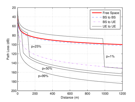
Figure 11: Path loss.

IV-B BS-BS Interference

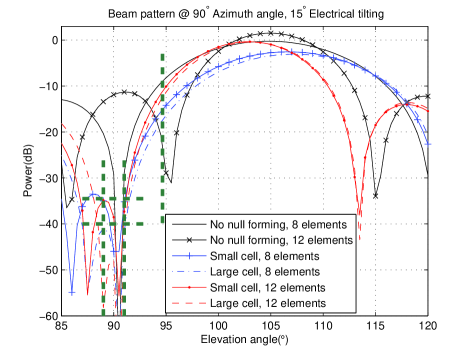
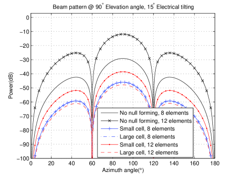
Figure 12: Beam patterns with and without null forming: (a) Elevation angle (b) Azimuth angle.

As discussed in Section I, with STR at BS, BS-BS interference is an extremely serious issue in cellular systems and overwhelms weak UL signal. Hence, serious loss of UL capacity is observed unless this interference is greatly reduced. In order to cope with BS-BS interference, we suggest a null forming in elevation angle at BS antennas. As tilting is employed at each BS and every BS has similar height, by simply creating nulls at the vicinity of $90^{\circ}$ in elevation angle, BS-BS interference can be avoided. First, we split each $4\lambda$ height antenna to eight $1/2\lambda$ elements vertically stacked. Notice that as the effective sizes of the antennas in the two configurations are equivalent, antenna gains will be unchanged. Since we have 4 elements horizontally, we have two dimensional $4\times 8$ antenna array. Assuming that $M\times N$ planar array is located at x-z plane facing toward positive y-axis with $1/2\lambda$ spacing of all elements, we have the following beam pattern

$$A(\theta,\phi)=$$

$$\left|\frac{1}{MN}\sum_{m=0}^{M-1}\sum_{n=0}^{N-1}w_{m,n}e^{jm\pi\sin(\theta)\cos(\phi)}e^{jn\pi\cos(\theta)}\right|^{2}A_{0}(\theta,\phi)$$ (33)

where $w_{m,n}$ is the weight for $(m,n)$-th element, $M$ is the number of horizontal elements, $N$ is the number of vertical elements, $\theta$ is elevation angle measured from positive z-axis, $\phi$ is azimuth angle measured from positive x-axis toward positive y-axis in x-y plane, and $A_{0}(\theta,\phi)$ is the beam pattern of $1/2\lambda$ height and $1/2\lambda$ width rectangular antenna element. By ignoring antenna coupling, etc., the following ideal beam pattern is obtained

$$A_{0}(\theta,\phi)=\left|Sinc\left(\frac{\cos(\theta)}{2}\right)Sinc\left(\frac{\sin(\theta)\cos(\phi)}{2}\right)\right|^{2}.$$ (34)

The above pattern (IV-B) is used for $0\leq\phi,\theta\leq\pi$ and scaled down by 25 dB for the backlobe ($\phi>\pi$). Although we can make a null at an arbitrary azimuth and elevation angle, we create a null at particular elevation angle over the entire range of azimuth angle for simplicity. Therefore, the weight $w_{m,n}$ can be split into horizontal and vertical weights as shown below

$$w_{m,n}=w_{m}^{h}w_{n}^{v}$$ (35)

where superscript $(\cdot)^{h}$ and $(\cdot)^{v}$ represent horizontal and vertical weight, respectively. The horizontal weights $\{w_{m}^{h}\}$ come from conventional closed-loop or open-loop MIMO techniques. In this paper without loss of generality we assume $w_{m}^{h}=1$. With $15^{\circ}$ electrical down tilting, the vertical weights become

$$w_{n}^{v}=e^{-jn\pi\cos(105\pi/180)}.$$ (36)

In order to create nulls MMSE beamforming is used. Then, the following row vector creates nulls toward $\{\theta_{k},k\neq 0\}$ while maintaining main beam direction $\theta_{0}$

$$\textbf{{w}}^{v}=\textbf{{a}}^{H}(\theta_{0})\left(\textbf{{a}}(\theta_{0})\textbf{{a}}^{H}(\theta_{0})+\sum_{k\neq 0}\textbf{{a}}(\theta_{k})\textbf{{a}}^{H}(\theta_{k})+\epsilon\textbf{{I}}\right)^{-1}$$ (37)

where $\textbf{{a}}(\theta_{0})=[1~{}e^{j\pi\cos(\theta_{0})}~{}\cdots e^{j(N-1)\pi\cos(\theta_{0})}]^{T}$ is an array vector toward main beam direction $\theta_{0}$, $\epsilon$ controls the depth of nulls, and superscript $(\cdot)^{H}$ represents complex conjugate transpose. We normalize the weight vector by maximum magnitude of its elements so that the magnitude of any element does not exceed 1

$$\textbf{{w}}^{v}=\textbf{{w}}^{v}/\max_{n}|w_{n}^{v}|.$$ (38)

The above normalization is more practical in transmit beamforming than finite norm of the weight vector although some loss of power is expected in transmission mode. The null forming is applied to both transmit and receive beam, which will relax the requirement on the depth of nulls. We create wide nulls from $89^{\circ}$ to $91^{\circ}$ for 25 m high BS antennas to allow variation of antenna heights from 16.3 m to 33.7 m at neighboring BSs located at 500 m distance.

Fig. 12 (a) illustrates beam patterns with and without null forming as a function of elevation angle at $90^{\circ}$ azimuth angle. With $15^{\circ}$ electrical tilting, the beam pattern of 12 antenna elements without null forming has high gain at around $90^{\circ}$ elevation angle. However, the beam of 8 antenna elements has a null at $90.5^{\circ}$. Hence, by changing the tilting angle to $14.5^{\circ}$, the null points to $90^{\circ}$. Unfortunately, the null is not wide enough to accommodate the variation of the antenna heights. Hence, for wider nulls, we apply the proposed technique to both 8 and 12 antenna elements. Two vertical lines around $90^{\circ}$ in the Fig. 12 (a) show the range of nulls and two horizontal lines represent the targets on the depth of nulls for the small and large cell. Since the transmit power in the small cell is 23 dB smaller while the path loss from the first tier BSs is 12.3 dB smaller, the requirement on the depth of nulls is looser in the small cell. Vertical line at $94.65^{\circ}$ represents the elevation angle pointing to cell edge UEs. Due to null forming we observe some loss in signal power especially at cell edge. One option to fix this is to reduce the cell size. Since the path loss exponent of BS-BS channel is smaller than that of BS-UE channel, reducing the cell size will help to improve cell edge performance. Also by increasing the number of antenna elements we can overcome the loss to certain extent as seen in the Fig. 12 (a). From $90^{\circ}$ to $94.65^{\circ}$ it is noticeable that the gain of beam due to null forming is smaller than the gain of the beam pattern without null forming. Thus, it reduces the co-channel interference to and from neighboring cells. Due to the reduction in interference power, although the signal power is reduced due to null forming, in interference limited systems not much loss of capacity is observed at cell edge, and a gain in cell center is possible. Fig. 12 (b) shows the beam patterns as a function of azimuth angle at $90^{\circ}$ elevation angle. It is clear that over entire range of horizontal angle the beams with null forming meet the requirements on the depth of nulls. Due to the assumption of 25 dB backlobe rejection, null forming and 40 dB path loss at 1 m, BS-BS interferences between sectors at the same site is negligible as well.

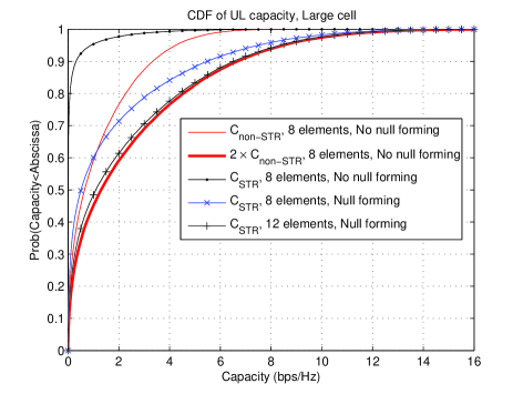
Figure 13: CDF of UL capacity in large cell.

Fig. 13 depicts the CDFs of UL capacity with various weight vectors in the large cell. The large cell is worse than the small cell regarding BS-BS interference especially in cell edge performance. Thus, we show the CDFs of the large cell. In order to simulate various antenna heights, we randomly choose BS-BS angle between $89^{\circ}$ and $91^{\circ}$. Throughout this paper we treat non-STR system as a reuse 2 system since DL and UL require separate non-overlapping resources. Therefore, we divide non-STR capacity by two. As seen in Fig. 13, due to BS-BS interference, STR exhibits serious loss of capacity unless null forming is employed. When null forming is employed, the CDF of STR capacity approaches twice the non-STR capacity. Although due to null forming some loss in signal power is observed, this loss can be overcome by reducing the cell size without changing the transmit power and antenna gain, or by increasing the number of antenna elements.

IV-C UE-UE Interference

The significance of UE-UE interference depends on its power relative to BS-UE interference power. With random choice of $p$ in each UE-UE link in the range of $25\%<p<99\%$, we observed that UE-UE interference is more severe than BS-UE interference in the small cell but weaker in the large cell. Hence, we can ignore UE-UE interference in the large cell since BS-UE interference is more dominant. Fig. 14 demonstrates the gain of DL capacity including UE-UE interference impact when $25\%<p<99\%$. Clearly, STR achieves twice of non-STR capacity almost everywhere. Note that the STR capacity with null forming can be better than twice of non-STR capacity. This comes from the fact that null forming reduces co-channel interference. Thus, in the interference limited system, when null forming is employed, the capacity of STR can be more than double of non-STR capacity except at cell edge. The cell edge performance can be improved by adjusting the cell size to compensate the signal power loss due to null forming. When UE-UE channel model is favorable, STR combined with null forming results in significant gains in both DL and UL.

However, it is obvious that when UE-UE path loss is smaller than BS-UE path loss, UE-UE interference will be more dominant than BS-UE interference. In the small cell the distance between UEs becomes smaller as the cell radius is 70.6 m. As it can be observed from Fig. 11, when $p=25\%$, in distances up to 115 m, UE-UE channel is LoS and its path loss is always much less than the one for BS-UE. For example at 115 m, UE-UE path loss is 75 dB while BS-UE path loss is 113 dB even though BS has higher antenna height than UE. Thus, UE-UE interference is more dominant in small cell in this setting. In practice there is a correlation between BS-UE and UE-UE channel model. When UE-UE channel has high chance of LoS, BS-UE may also have high chance of LoS. However, due to lack of channel models that include such correlation, we study the system level performances with various values of $p$ to simulate different environments.

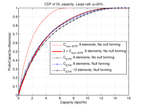
Figure 14: CDF of DL capacity in large cell.

It is apparent that coordination over multiple cells can reduce UE-UE interference by joint scheduling. For example, when two UEs see strong UE-UE interference from each other, scheduler can schedule them in orthogonal resources. There is no doubt that through the coordination, UE-UE interference can be avoided. The UE-UE interference from neighboring sectors at sector boundary is also considerably significant in reuse 1. Since a coordination between sectors from the same site is relatively easier, the coordination in the same site is quite feasible. In addition aggregating multiple BSs at one physical signal processing center is being developed called Cloud Radio Access Network (C-RAN) which makes the coordination easier. Recently, a coordination among multiple BSs has been defined in 3GPP [21]. By exchanging location information of UEs among neighboring BSs, to some degree we can avoid UE-UE interference as well. In general, some form of coordination will be made available in near future.

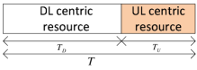
Figure 15: Basic resource block structure for UE-UE interference reduction.

However, in this work, for the sake of simplicity we focus on a technique which does not require any coordination. Under this constraint, there is no other way than turning off some UEs’ UL transmissions which create severe UE-UE interferences to other UEs. Thus, DL capacity can be improved at the cost of UL capacity. For this end, we start off with half duplex. A basic resource block is suggested in Fig. 15 where the resource block is split into two parts. One for DL centric resource with size of $T_{D}$ and the other for UL centric resource with size of $T_{U}$. Note that a packet is transmitted using multiple of the basic resource blocks. During the DL centric resource, UEs which can benefit from additional UL transmission by STR are selected for STR operation. This additional UL will be a gain in UL capacity but it creates UE-UE interferences to the DL signals in other cells. Obviously the additional UL gain should be larger than the DL loss. Due to the assumption of no coordination, we simply check DL signal power-to-interference and noise power ratio (SINR) in order to choose STR enabled UEs during the DL resource. Likewise, over the UL duration, we search UEs which can provide net gain by enabling DL transmission using STR. The DL signal for the STR UE will not interfere with UL signals due to null forming at BS. However, it creates conventional DL co-channel interference to other DL signals in neighboring cells.

Unlike DL co-channel interference from BS to UE, UE-UE interference is dependent on the locations of other UEs. Thus, information on which UEs are scheduled in other BSs is necessary. We need to address how to obtain DL SINR that includes UE-UE interferences without knowing the scheduling decisions of neighboring BSs. We suggest the following: first, each BS schedules UE. Then, the scheduled UE sends UL pilots without sending data yet. Using the UL Pilots, the UE measures the interferences from other UEs in co-channel BSs. Then, the UE calculates DL SINR assuming STR operation in all UEs. Afterwards, each UE reports the DL SINR to the home BS. If the DL SINR is lower than a certain threshold, UE is scheduled to operate in non-STR mode in successive resource. Otherwise, it is scheduled to operate in STR mode. The thresholds for DL and UL centric resources may be different in general. In addition, by optimizing the amount of resources assigned to DL and UL centric zones, capacity can be further improved. Thus, we have three dimensional optimization problem. The proposed resource block structure provides good flexibility between DL and UL capacity.

TABLE V: Improvement of capacity over non-STR with 8 antennas and no null forming: Large cell

Number	DL						UL
of	$p>$0.25		$p>$0.37		$p>$0.5
Antennas	Mean	Edge	Mean	Edge	Mean	Edge	Mean	Edge
8	100.6%	-35.0%	103.0%	0.2%	103.8%	17.5%	42.8%	-50.0%
12	116.8%	2.2%	119.3%	46.7%	120.1%	66.7%	90.9%	32.8%

TABLE VI: Improvement of capacity over non-STR with 8 antennas and no null forming: Small cell

Number	DL				UL
of	$p>$0.25		$p>$0.37
Antennas	Mean	Edge	Mean	Edge	Mean	Edge
8	37.7%	-92.6%	69.8%	-80.9%	55.8%	-27.5%
12	55.3%	-82.4%	84.8%	-59.7%	83.5%	36.2%

TABLE VII: Improvement of capacity over non-STR with 8 antennas and no null forming: Small cell, using the resource block structure

Number	DL				UL
of	$p>$0.25		$p>$0.37		$p>$0.25		$p>$0.37
Antennas	Mean	Edge	Mean	Edge	Mean	Edge	Mean	Edge
8	64.6%	2.0%	81.1%	-0.9%	0.2%	-53.2%	27.9%	-45.7%
12	71.3%	6.9%	92.1%	17.1%	44.6%	8.4%	63.7%	16.3%

However, one difficulty in solving this optimization problem is the lack of a well-known cost function that can capture gains in cell edge and cell average in both DL and UL. In general different cost functions can be considered depending on the application and the required gain in each parameter. Here, our objective is to simply maximize the sum of all gains i.e., DL cell edge gain + UL cell edge gain + DL cell average gain + UL cell average gain.

Table V-VII show gains in average and 5% cell edge capacity of STR with null forming over non-STR with 8 antennas without null forming. First, consider the large cell. As discussed earlier in this case, UE-UE interference is not a serious problem. It can be seen from Table V that more than 100% of gain in DL cell average capacity can be achieved by STR with null forming in both 8 and 12 antennas and decent gain in cell edge with 12 antennas. The gains beyond 100% in cell average come from the reduction of DL co-channel interference due to null forming. However, since UL is less interference limited, the gain is smaller. The cell edge capacity is not close to twice of non-STR capacity since the signal power loss is unavoidable at cell edge due to null forming.

Next, let us consider the case where UE-UE interference is more dominant than DL co-channel interference i.e. small cell with small $p$. As it can be observed from Table VI, without addressing UE-UE interference, cell edge users experience serious loss in DL capacity. Nevertheless, by employing the proposed resource block structure and optimizing above cost function, positive gains can be achieved with STR and 12 antennas by sacrificing UL capacity as shown in Table VII.

Although we assumed that each UE uses the whole bandwidth for time division multiplexing (TDM), it is possible to allocate fraction of bandwidth to each UE for frequency division multiplexing (FDM). Then, UE-UE interference will be larger unless the power spectral density is maintained the same. In addition, due to proximate UEs, in the same sector higher resolution ADC will be needed. Due to path loss, the saturation at LNA can be avoided.

V Conclusions

We have suggested an echo cancellation technique which can be implemented in analogue domain and demonstrated sufficient suppression of echo before LNA. The technique is robust to RF impairments exhibiting outstanding performance without requiring additional antennas.

STR can be employed in CSMA networks. We showed that STR can reduce the hidden node problem and the suggested protocols improve throughput in both single and multiple cells. The application of STR to cellular systems creates BS-BS and UE-UE interferences. We have provided a solution for the complete cancellation of BS-BS interference. For UE-UE interference, we studied non-cooperative method.

Appendix A

First, we define normalized correlation as

$$\textbf{{r}}_{{}_{Y\textbf{{X}}}} =\frac{1}{P}E\{X(t-\tau)[X^{*}(t-\tau_{1})~{}X^{*}(t-\tau_{2})]\}$$

$$=[Sinc(B(\tau-\tau_{1}))~{}Sinc(B(\tau-\tau_{2}))]$$ (A.1)

where $P$ is the average power of $X(t)$. Similarly, define normalized auto-correlation as

$$\textbf{{r}}_{{}_{\textbf{{XX}}}}=\frac{1}{P}$$

$$\left[{{\begin{array}[]{*{2}c}E\{X(t-\tau_{1})X^{*}(t-\tau_{1})\}&E\{X(t-\tau_{1})X^{*}(t-\tau_{2})\}\\ E\{X(t-\tau_{2})X^{*}(t-\tau_{1})\}&E\{X(t-\tau_{2})X^{*}(t-\tau_{1})\}\\ \end{array}}}\right]$$ (A.4)

$$= \left[{{\begin{array}[]{*{2}c}1&Sinc(B(\tau_{1}-\tau_{2}))\\ Sinc(B(\tau_{2}-\tau_{1}))&1\\ \end{array}}}\right].$$ (A.7)

Then, the cross correlation vector can be written as

$$\textbf{{R}}_{YX}=E\{Y(t)\textbf{{X}}^{H}(t)\}=ge^{j\omega\tau}P\textbf{{r}}_{{}_{Y\textbf{{X}}}}\textbf{{D}}$$ (A.8)

where D is a diagonal matrix defined as

$$\textbf{{D}}=\left[{{\begin{array}[]{*{2}c}e^{-j\omega\tau_{1}}&0\\ 0&e^{-j\omega\tau_{2}}\\ \end{array}}}\right].$$ (A.9)

Likewise, the auto-correlation matrix can be expressed as

$$\textbf{{R}}_{XX}=E\{\textbf{{X}}(t)\textbf{{X}}^{H}(t)\}=P\textbf{{D}}^{*}\textbf{{r}}_{{}_{\textbf{{XX}}}}\textbf{{D}}.$$ (A.10)

The weight vector for the Wiener solution is obtained by

$$\textbf{{W}}^{T}=\textbf{{R}}_{YX}\textbf{{R}}_{XX}^{-1}=ge^{j\omega\tau}\textbf{{r}}_{{}_{Y\textbf{{X}}}}\textbf{{r}}_{{}_{\textbf{{XX}}}}^{-1}\textbf{{D}}.$$ (A.11)

After manipulations, the residual echo power defined in the denominator of (12) is in the form of

$$E\{|gX(t-\tau)e^{j\omega\tau}-\textbf{{W}}^{T}\textbf{{X}}(t)|^{2}\}=g^{2}P-g^{2}P\textbf{{r}}_{{}_{Y\textbf{{X}}}}\textbf{{r}}_{{}_{\textbf{{XX}}}}^{-1}\textbf{{r}}_{{}_{Y\textbf{{X}}}}^{H}.$$ (A.12)

Finally, the suppression level of echo power (11) is calculated from

$$\text{Suppression}=\frac{1}{1-\textbf{{r}}_{{}_{Y\textbf{{X}}}}\textbf{{r}}_{{}_{\textbf{{XX}}}}^{-1}\textbf{{r}}_{{}_{Y\textbf{{X}}}}^{H}}.$$ (A.13)

Appendix B

In order to give some insight on how phase noise affects the performance, without loss of generality, the following simplified model is considered. We consider one echo and assume ideal knowledge of the delay. With one tap echo canceller and zero valued weight initially, we have

$$Z(t)=HX(t)$$ (B.1)

where $H=|H|e^{j\theta_{h}}$ is the echo channel response. The echo channel estimation for in-phase which drives the weight is

$$Re\{X^{*}(t)Z(t)\}=|H||X(t)|^{2}cos(\theta_{h}).$$ (B.2)

Ideally, the weight should converge to

$$w=|H|cos(\theta_{h}).$$ (B.3)

However, the echo channel estimation (B.2) is far from $|H|cos(\theta_{h})$ unless it is divided by $|X(t)|^{2}$. In addition, the echo channel estimation will be corrupted by noise and various impairments. Note also that random OFDM signal $X(t)$ has large peak-to-average power ratio (PAPR). Hence, in adaptive echo canceller, the echo channel estimation is low-pass filtered by an integrator with very small step-size $\mu$ as the echo channel estimation is quite noisy. Thus, the estimation error in echo channel estimation does not directly appear in the weight. As far as the sign of $Re\{X^{*}(t)Z(t)\}$ is equal to the sign of true echo channel $|H|cos(\theta_{h})$, the weight will be gradually updated toward the true echo channel until the power of $Z(t)$ is small enough. Due to this nature, even if the echo channel estimation is not perfect and corrupted by impairments and noise, the adaptive echo canceller can converge.

$$Re\{\tilde{X}^{*}(t)\tilde{Z}(t)e^{j\Delta}\}=\frac{|H||X(t)|^{2}}{2} \left\{\left[\cos(\theta_{h})\left\{\begin{array}[]{l}g_{x,i}g_{z,i}(\cos(\delta_{i-i}+\varepsilon_{x-z}(t))+\cos(2\theta_{x}(t)-\delta_{i+i}-\varepsilon_{x+z}(t)))+\\ g_{x,q}g_{z,q}(\cos(\delta_{q-q}+\varepsilon_{x-z}(t))-\cos(2\theta_{x}(t)-\delta_{q+q}-\varepsilon_{x+z}(t)))\end{array}\right\}\right.\right.$$ (B.15)

$${-}\>\left.\sin(\theta_{h})\left\{\begin{array}[]{l}g_{x,i}g_{z,i}(\sin(\delta_{i-i}+\varepsilon_{x-z}(t))+\sin(2\theta_{x}(t)-\delta_{i+i}-\varepsilon_{x+z}(t)))+\\ g_{x,q}g_{z,q}(\sin(\delta_{q-q}+\varepsilon_{x-z}(t))-\sin(2\theta_{x}(t)-\delta_{q+q}-\varepsilon_{x+z}(t)))\end{array}\right\}\right]\cos(\Delta)$$

$${-}\!\left[\cos(\theta_{h})\left\{\begin{array}[]{l}g_{x,i}g_{z,q}(\sin(\delta_{i-q}+\varepsilon_{x-z}(t))+\sin(2\theta_{x}(t)-\delta_{i+q}-\varepsilon_{x+z}(t)))+\\ g_{x,q}g_{z,i}(\sin(\delta_{q-i}+\varepsilon_{x-z}(t))-\sin(2\theta_{x}(t)-\delta_{q+i}-\varepsilon_{x+z}(t)))\end{array}\right\}\right.$$

$${+}\>\left.\left.\sin(\theta_{h})\left\{\begin{array}[]{l}g_{x,i}g_{z,q}(\cos(\delta_{i-q}+\varepsilon_{x-z}(t))+\cos(2\theta_{x}(t)-\delta_{i+q}-\varepsilon_{x+z}(t)))+\\ g_{x,q}g_{z,i}(\cos(\delta_{q-i}+\varepsilon_{x-z}(t))-\cos(2\theta_{x}(t)-\delta_{q+i}-\varepsilon_{x+z}(t)))\end{array}\right\}\right]\sin(\Delta)\right\}.$$

$$E\{Re\{\tilde{X}^{*}(t)\tilde{Z}(t)e^{j\Delta}\}\}=\frac{e^{-\sigma^{2}}|H|P}{2}$$

$$\;\;\left\{\left[\cos(\theta_{h})\left\{g_{x,i}g_{z,i}\cos(\delta_{i-i})+g_{x,q}g_{z,q}\cos(\delta_{q-q})\right\}-\sin(\theta_{h})\left\{g_{x,i}g_{z,i}\sin(\delta_{i-i})+g_{x,q}g_{z,q}\sin(\delta_{q-q})\right\}\right]\cos(\Delta)\right.$$

$$\left.-\left[\cos(\theta_{h})\left\{g_{x,i}g_{z,q}\sin(\delta_{i-q})+g_{x,q}g_{z,i}\sin(\delta_{q-i})\right\}+\sin(\theta_{h})\left\{g_{x,i}g_{z,q}\cos(\delta_{i-q})+g_{x,q}g_{z,i}\cos(\delta_{q-i})\right\}\right]\sin(\Delta)\right\}.$$ (B.17)

Now, let us add all impairments such as phase/amplitude imbalance and phase noise. The phase noise difference and sum between downconverters for $X(t)$ and $Z(t)$ are defined by

$$\varepsilon_{x-z}(t)=\varphi_{x}(t)-\varphi_{z}(t),\varepsilon_{x+z}(t)=\varphi_{x}(t)+\varphi_{z}(t).$$

Define the phase imbalance difference and sum of in-phase and quadrature phase between downconverters for $X(t)$ and $Z(t)$ as following

$$\delta_{i-i}=\phi_{x,i}-\phi_{z,i},\delta_{q-q}=\phi_{x,q}-\phi_{z,q},$$

$$\delta_{i+i}=\phi_{x,i}+\phi_{z,i},\delta_{q+q}=\phi_{x,q}+\phi_{z,q},$$

$$\delta_{i-q}=\phi_{x,i}-\phi_{z,q},\delta_{q-i}=\phi_{x,q}-\phi_{z,i},$$

$$\delta_{i+q}=\phi_{x,i}+\phi_{z,q},\delta_{q+i}=\phi_{x,q}+\phi_{z,i}.$$

Then, the echo channel estimation can be written as shown in (B.15) where $\theta_{x}(t)$ is the angle of $X(t)$ assuming uniformly distributed over $0$ to $2\pi$ and $\Delta$ is the phase difference between downconverters for $Z(t)$ and $X(t)$. When in majority of samples the sign of $Re\{\tilde{X}^{*}(t)\tilde{Z}(t)\}$ is equal to the sign of $|H|cos(\theta_{h})$, the weight will be updated to the right direction.

Due to random time varying phase from transmitted signal $\theta_{x}(t)$, phase noise $\varphi_{x}(t)$ and $\varphi_{z}(t)$, the echo channel estimation will fluctuate. However, by the low pass filtering, those time varying noises will be filtered. Since we can assume the phase noise and the phase of transmitted signal are stationary, the integration over time can effectively perform ensemble average. Assuming Gaussian phase noise, the ensemble average over $X(t)$, $\varphi_{x}(t)$ and $\varphi_{z}(t)$ leads to (Appendix B) where $\sigma^{2}$ is the variance of phase noise and $P$ is the average power of $X(t)$. As can be seen, the phase noise reduces the power of echo channel estimation. Hence, the performance will be more sensitive to the noise. When all downconverters are driven by the same oscillator, the phase noises can be identical. In this scenario, the phase noise difference $\varepsilon_{x-z}(t)$ will be zero. Then, the scale factor $e^{-\sigma^{2}}$ disappears as if no phase noise is present.

Yang-Seok Choi (S’91,M’01) received the B.S. degree from Korea University, Seoul, Korea, in 1990, the M.S.E.E. degree from Korea Advanced Institute of Science and Technology (KAIST), Taejon, Korea, in 1992, and the Ph.D. degree from Polytechnic University, Brooklyn, NY, USA in 2000, all in electrical engineering. From 1992 to 1996, he was with Samsung Electronics, Co., Ltd., Suwon, Korea, where he developed various modems for HDTV and DBS. During 2000 summer he held a Summer intern position at AT&T Labs-Research Shannon Lab, Florham Park, NJ, USA. In 2000, he joined National Semiconductor, East Brunswick, NJ, USA where he was involved in the development of W-CDMA. During 2001-2002, he was a Senior Technical Staff Member at AT&T Labs-Research, Middletown, NJ, USA where he researched on MIMO systems, OFDM systems and information theory. From 2002 to 2004 he had been with ViVATO, Inc., Spokane, WA, USA working on MIMO OFDM systems, smart antenna systems, and antenna/beam selection techniques. In 2004, he joined Intel Corporation, Hillsboro, OR, USA where he studied on broadband wireless communications systems and was a director of Radio Systems Engineering leading Standards and technology development. In 2013, he joined Intel Labs where he researches future generation wireless systems. His research interests include various aspects of wireless communications systems.

Hooman Shirani-Mehr (S’03- M’10) received the B.S. degree from Sharif University of Technology, Tehran, Iran, in 2001 and M.S. and Ph.D. degrees from the University of Southern California, Los Angeles, CA in 2006 and 2010, respectively, all in electrical engineering. Since 2010, he has been with Intel Corporation where he is currently working on 3GPP LTE and LTE-Advanced wireless systems. His research interests include communication theory, information theory and signal processing with applications in wireless communications.

References

- [1] J. I. Choi, M. Jain, K. Srinivasan, P. Levis and S. Katti, “Achieving single channel, full duplex wireless communication”, Proceedings of the 16th Annual International Conference on Mobile Computing and Networking, pp. 1-12, Sep. 2010.
- [2] S. Hong, J. Mehlman, and S. Katti, “Picasso: Flexible RF and Spectrum Slicing”, SIGCOMM, pp. 283-284, Aug. 2012.
- [3] S. Chen, M.A. Beach, J.P. McGeehan, “Division-free duplex for wireless applications”, IEEE Electron. Lett., vol. 34, No. 2, pp. 147-148, Jan. 1998.
- [4] S. Kannangara and M. Faulkner, “Adaptive Duplexer for Multiband Transreceiver”, Proceedings of Radio and Wireless Conference, pp. 381-384, Aug. 2003.
- [5] Intersil Inc., “QHX220 narrowband noise canceller IC”, http://www.intersil.com/products/deviceinfo.asp?pn=QHX220.
- [6] Y. Hua, P. Liang, Y. Ma, A. C. Cirik, and Q. Gao, “A Method for Broadband Full-Duplex MIMO Radio”, IEEE Trans. Signal Process. Lett., vol. 19, No. 12, pp. 793-796, Dec. 2012.
- [7] E. Aryafar, M. A. Khojastepour, K. Sundaresan, S. Rangarajan, and M. Chiang, “MIDU: Enabling MIMO Full Duplex”, Proceedings of ACM MobiCom, Istanbul, Turkey, 2012.
- [8] M. Jain et al., “Practical, Real-time, Full Duplex Wireless”, Proceedings of the 17th Annual International Conference on Mobile Computing and Networking, 2011.
- [9] M. Duarte and A. Sabharwal, “Full-duplex wireless communications using off-the-shelf radios : Feasibility and First results”, Proceedings of Asilomar Conference on Signals, Systems and Computers, pp. 1558-1562, Nov. 2010.
- [10] A. Sahai, G. Patel and A. Sabharwal, “Pushing the limits of full duplex : Design and Real-time implementation”, Rice University Technical Report TREE1104, Jul. 2011.
- [11] N. Singh, D. Gunawardena, A. Proutiere, B. Radunovic, H. V. Balan, and P. Key, “ Efficient and fair MAC for wireless networks with self-interference cancellation”, International Symposium on Modeling and Optimization in Mobile, Ad Hoc and Wireless Networks, pp. 94 - 101, May 2011.
- [12] RFMD Inc., “RFSA2013 Data Sheet”, http://www.rfmd.com/CS/Documents/RFSA2013DS.pdf.
- [13] S. Haykin, Adaptive Filter Theory, 3rd edition, Prentice-Hall, New Jersey, 1996.
- [14] A. Sahai, G. Patel, C. Dick and A. Sabharwal, “Understanding the Impact of Phase Noise on Active Cancellation in Wireless Full-Duplex”, Proceedings of Asilomar Conference on Signals, Systems and Computers., pp. 29-33, 2012.
- [15] T. O’Sullivan, R. A. York, B. Noren, and P. M. Asbeck, “Adaptive Duplexer Implemented Using Single-Path and Multipath Feedforward Techniques With BST Phase Shifters”, IEEE Trans. Microw. Theory Techn., vol. 53, No. 1, pp. 106-114, Jan. 2005.
- [16] Motia Inc., “Wi-Fi Beamforming IC BFA166”, http://www.motia.com/ufiles/Library/BFA166-v0.5.pdf.
- [17] J. Wang, J. Winters, M. C. Doong and C. C. Yang, “Wireless Communication System using a plurality of antenna elements with adaptive weighting and combining techniques”, US Patent 7,260,370, Aug., 2007.
- [18] L. Kleinrock and F. A. Tobagi, “Packet Swithching in Radio Channels: Part I- Carrier Sense Multiple-Access Modes and Their Throughput-Delay Characteristics”, IEEE Trans. on Commun., vol. 23, No. 12, pp. 1400-1416, Dec. 1975.
- [19] 3GPP TR 25.814, “3rd Generation Partnership Project; Technical Specification Group Radio Access Network; Physical layer aspects for evolved Universal Terrestrial Radio Access (UTRA) (Release 7)”, V7.1.0, 2006-09.
- [20] Report ITU-R M.2146, “Coexistence between IMT-2000 CDMA-DS and IMT-2000 OFDMA-TDD-WMAN in the 2 500-2 690 MHz band operating in adjacent bands in the same area”, 05/2009.
- [21] 3GPP TR 36.819, “3rd Generation Partnership Project; Technical Specification Group Radio Access Network; Coordinated multi-point operation for LTE physical layer aspects (Release 11)”, V11.1.0, 2011-12.