Electron-acoustic solitary pulses and double layers in multi-component plasmas

Abstract

We consider the nonlinear propagation of finite amplitude electron-acoustic waves (EAWs) in multi-component plasmas composed of two distinct groups of electrons (cold and hot components), and non-isothermal ions. We use the continuity and momentum equations for cold inertial electrons, Boltzmann law for inertialess hot electrons, non-isothermal density distribution for hot ions, and Poisson’s equation to derive an energy integral with a modified Sagdeev potential (MSP) for nonlinear EAWs. The MSP is analyzed to demonstrate the existence of arbitrary amplitude EA solitary pulses (EASPs) and EA double layers (EA-DLs). Small amplitude limits have also been considered and analytical results for EASPs and EA-DLs are presented. The implication of our results to space and laboratory plasmas is briefly discussed.

I Introduction

The idea of the electron-acoustic wave (EAW) has been conceived by Fried and Gould Fried1961 during numerical solutions of the linear electrostatic Vlasov dispersion equation in a uniform unmagnetized plasma. It is basically an acoustic-type waves Watanabe1977 , in which inertia is provided by the cold electron mass, and the restoring force comes from the hot electron thermal pressure. The ions play the role of a neutralizing background only. The spectrum of the linear EA waves, unlike that of the well-known Langmuir waves, extends only up to the cold electron plasma frequency $\omega_{pc}=(4\pi n_{c0}e^{2}/m_{e})^{1/2}$, where $n_{c0}$ is the unperturbed cold electron number density, $e$ magnitude of the electron charge, and $m_{e}$ the mass of the electron. This upper wave frequency limit $(\omega\simeq\omega_{pc})$ corresponds to a short-wavelength EAW and depends on the unperturbed cold electron number density $n_{c0}$. On the other hand, the dispersion relation of the linear EAWs in the long-wavelength limit [in comparison with the hot electron Debye radius $\lambda_{dh}=(k_{B}T_{h}/4\pi n_{h0}e^{2})^{1/2}$, where $T_{h}$ is the hot electron temperature, $k_{B}$ is the Boltzmann constant, and $n_{h0}$ the unperturbed hot electron number density] is $\omega\simeq kC_{e}$, where $k$ is the wave number and $C_{e}=(n_{c0}k_{B}T_{h}/n_{h0}m_{e})^{1/2}$ the EA speed Gary1985 . Besides the well-known Langmuir and ion-acoustic waves, they noticed the existence of a heavily damped acoustic-like solution of the dispersion equation. It was later shown that in the presence of two distinct groups (cold and hot) of electrons and immobile ions, one indeed obtains a weakly damped EAW Watanabe1977 , the properties of which significantly differ from those of the Langmuir waves. Gary and Tokar Gary1985 performed a parameter survey and found conditions for the existence of the EAWs. The most important condition is $T_{c}\ll T_{h}$, where $T_{c}$ $(T_{h})$ is the temperature of cold (hot) electrons. The propagation characteristics of the EAWs has also been studied by Yu and Shukla Yu1983 , Mace and Hellberg Mace1990 ; Mace1993 ; Mace2001 and Mace et al. Mace1991 .

Two-electron-temperature plasmas are known to occur both in laboratory experiments Derfler1969 ; Henry1972 ; Sheridan1991 ; Pickett2008 ; Kakad2009 ; Moon2010 ; Singh2011 ; Mondal2012 and in space environments Dubouloz1991 ; Dubouloz1993 ; Pottelette1999 ; Berthomier2000 ; Singh2001 . The propagation of the EAWs has received a great deal of renewed interest not only because the two-electron-temperature plasma is very common in laboratory experiments and in space, but also because of the potential importance of the EAWs in interpreting electrostatic component of the broadband electrostatic noise (BEN) observed in the cusp of the terrestrial magnetosphere Tokar1984 ; Singh2001 , in the geomagnetic tail Schriver1989 , in auroral region Dubouloz1991 ; Dubouloz1993 ; Pottelette1999 , etc.

The EAWs have been used to explain various wave emissions in different regions of the Earth’s magnetosphere Dubouloz1991 ; Dubouloz1993 . It was first applied to interpret hiss-emissions observed in the polar cusp region in association with low-energy $(\sim 100~{}eV)$ upward moving electron beams Lin1984 . The EAWs were also utilized to interpret the generation of the BEN emissions detected in the plasma sheath Schriver1989 , as well as in the dayside auroral zone Dubouloz1991 ; Dubouloz1993 . Dubouloz et al. Dubouloz1991 rigorously studied the BEN observed in the dayside auroral zone and showed that because of the very high electric field amplitudes $(100~{}mV/m)$ involved, the nonlinear effects must play a significant role in the generation of the BEN in the dayside auroral zone. Dubouloz et al. Dubouloz1991 ; Dubouloz1993 also explained the short-duration $(<1s)$ burst of the BEN in terms of electron acoustic solitary waves (EA-SWs): such EA-SWs passing the satellite would generate electric field spectra. To study the properties of EA solitary structures, Dubouloz et al. Dubouloz1991 considered a one-dimensional, unmagnetized collisionless plasma consisting of cold electrons, Maxwellian hot electrons, and stationary ions. El-Shewy El-Shewy2007 has investigated the propagation of linear and nonlinear EA-SWs in a plasma containing cold electrons, nonthermal hot electrons, and stationary ions. The effects of arbitrary amplitude EA-SWs and electron-acoustic double layers (EA-DLs) in a plasma consisting of cold electrons, superthermal hot electrons, and stationary ions has been considered by Sahu Sahu2010 . The EA-SWs in a two-electrons-temperature plasma where ions form stationary charge neutral background has been observed by Dutta Dutta2011 . El-Wakil et al. El-Wakil2011 considered cold electrons, nonthermal hot electrons, and stationary ions, and studied the nonlinear properties of EA-SWs by using time-fractional Korteweg-de Vries (K-dV) equation. On the other hand, there are some space, where the energetic ions are observed, and ion-temperature can very high, even higher than electron-temperature Lakhina2008 . The energetic ions are described by a nonthermal or Cairns et al. distribution Cairns1995 ; Mamun1996 ; Mamun2002 , and are referred to as nonthermal ions. The latter is now being common feature of the geospace plasmas, and in general it is turning out to be a characteristic feature of space plasmas Futaana2003 . For examples, nonthermal ions are observed in the Earth’s bow-shock region by the Vela satellite Asbridge1968 ; ASPERA on the Phobos 2 satellite has observed the loss of energetic ions from the upper ionosphere of Mars; in solar active region Imada2009 .

In this paper, we study the effect of non-thermal (energetic or fast) ions on small and large amplitude EA solitary pulses (EASPs) and EA-DLs in a multi-component plasma. It is found that the presence of non-isothermal ions greatly affect the features of both EASPs and EA-DLs. The latter can be identified as localized electrostatic excitations in observational data from space and laboratory plasmas.

II Governing Equations

We consider the nonlinear propagation of the EAWs in one-dimensional, collisionless, unmagnetized plasmas composed of cold electrons, hot electrons obeying a Boltzmann distribution, and nonthermal ions following nonthermal distribution. Thus, at equilibrium, we have $n_{c0}+n_{h0}=n_{i0}$, where $n_{i0}$ is the nonthermal ion number density at equilibrium. The nonlinear dynamics of the EAWs propagating in such a plasma system is governed by

$$\frac{\partial n_{c}}{\partial t}+\frac{\partial}{\partial x}(n_{c}u_{c})=0,$$ (1)

$$\frac{\partial u_{c}}{\partial t}+u_{c}\frac{\partial u_{c}}{\partial x}=\frac{\partial\Psi}{\partial x},$$ (2)

$$\frac{\partial^{2}\Psi}{\partial x^{2}}=\mu e^{\Psi}+(1-\mu)n_{c}-(1+\beta\sigma\Psi+\beta\sigma^{2}\Psi^{2})e^{-\sigma\Psi},$$ (3)

where $n_{c}$ is the cold electron number density normalized by its equilibrium value $n_{c0}$, $u_{c}$ the cold electron speed normalized by $C_{e}$, $\Psi$ the wave potential normalized by $k_{B}T_{h}/e$, $\mu=n_{h0}/n_{i0}$, $\sigma=T_{h}/T_{i}$, $T_{i}$ the ion temperature, and $\beta=4\alpha/(1+3\alpha)$, in which $\alpha$ is the nonthermal parameter Cairns1995 ; Mamun1996 ; Mamun2002 . The time variable $t$ is in units of $\omega^{-1}_{pc}$, and the space variable $x$ is normalized by $\lambda_{dh}$. Our three-component plasma model is valid for electrostatic disturbances with the EAW phase speed much larger (smaller) than the thermal speed of the cold electrons (hot electrons and hot ions). The non-isothermal ion density distribution is associated with an ion distribution function that departs from the Maxwell-Boltzmann law on account of the EA wave amplitude dependent of the ion energy in the nonlinear regime.

III Derivation of Energy Integral

To derive an energy integral Bernstein1957 ; Sagdeev1966 from Eqs. (1)-(3), we first make all the dependent variables to depend only on a single variable $\xi=x-Mt$, where $M$ is the nonlinear wave speed normalized by $C_{e}$. We note that $M$ is not the Mach number, since it is normalized by $C_{e}$, which is not the EAW phase speed. Now, using the steady-state condition and imposing the appropriate boundary conditions (namely, $n_{c}\rightarrow 1$, $u_{c}\rightarrow 0$, and $\Psi\rightarrow 0$ at $\xi\rightarrow\pm\infty$, one can express $n_{c}$ as

$$n_{c}=\left(1+\frac{2\Psi}{M^{2}}\right)^{-1/2}.$$ (4)

Now, substituting Eq. (4) into Eq. (3), multiplying the resulting equation by $d\Psi/d\xi$, and applying the boundary condition, $d\Psi/d\xi\rightarrow 0$ at $\xi\rightarrow\pm\infty$, one obtains an energy integral

$$\frac{1}{2}\left(\frac{d\Psi}{d\xi}\right)^{2}+V(\Psi)=0,$$ (5)

for an oscillating particle of unit mass, with pseudo-position $\Psi$, pseudo-time $\xi$, and a pseudo-potential $V(\Psi)$. The latter for our purposes reads

$$V(\Psi)=\mu(1-e^{\Psi})+(1-\mu)M^{2}\left(1-\sqrt{1+\frac{2\Psi}{M^{2}}}\right)$$

$$-\frac{e^{-\sigma\Psi}}{\sigma}\left(1+3\beta+3\beta\sigma\Psi+\beta\sigma^{2}\Psi^{2}\right)+\frac{1}{\sigma}(1+3\beta),$$ (6)

which is valid for the arbitrary amplitude EASPs and EA-DLs in our plasma.

IV Small Amplitude Results

We first investigate the properties of small amplitude EASPs and EA-DLs by using a pseudo-potential approach Bernstein1957 ; Sagdeev1966 . The expansion of $V(\Psi)$ around $\Psi=0$ is

$$V(\Psi)=C_{2}\Psi^{2}+C_{3}\Psi^{3}+C_{4}\Psi^{4}+\cdot\cdot\cdot\cdot,$$ (7)

where

$$C_{2}=\frac{1}{2}\left[\frac{1-\mu}{M^{2}}-\mu-\sigma(1-\beta)\right],$$ (8)

$$C_{3}=\frac{1}{6}\left[-\frac{3(1-\mu)}{M^{4}}-\mu+\sigma^{2}\right],$$ (9)

$$C_{4}=\frac{1}{24}\left[\frac{15(1-\mu)}{M^{6}}-\mu-\sigma^{3}(1+3\beta)\right].$$ (10)

IV.1 EA Solitary Pulses

Let us first consider small-amplitude EASPs for which $V(\Psi)=C_{2}\Psi^{2}+C_{3}\Psi^{3}+C_{4}\Psi^{4}$ holds. This approximation allows us to write the small-amplitude solitary wave solution Mannan2011 of Eq. (5) as

$$\Psi=\left[\frac{1}{\Psi_{m2}}-\left(\frac{1}{\Psi_{m2}}-\frac{1}{\Psi_{m1}}\right)\cosh^{2}\left(\frac{\xi}{\delta}\right)\right]^{-1},$$ (11)

where

$$\Psi_{m1,2}=\Psi_{m}\left[1\mp\sqrt{1-\frac{C_{2}}{C_{0}}}\right],$$

$$\Psi_{m}=-\frac{C_{3}}{2C_{4}},$$

$$\delta=\sqrt{-\frac{2}{C_{4}\Psi_{m1}\Psi_{m2}}},\$$

$\delta$ is the width of the EASPs, and $C_{0}=C_{3}^{2}/4C_{4}$.

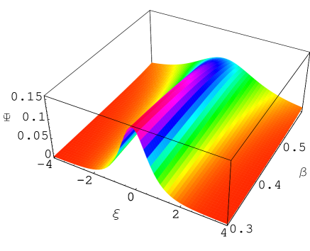
Figure 1: (Color online) Showing how the amplitude and the width of the positive EASPs vary with $\beta$ for $\sigma=10$, $\mu=0.5$, and $M=0.36$.

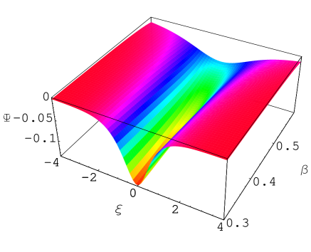
Figure 2: (Color online) Showing how the amplitude and the width of the negative EASPs vary with $\beta$ for $\sigma=10$, $\mu=0.5$, and $M=0.35$.

The profiles (indicating the amplitude and width) of the small amplitude EASPs associated with positive and negative potential are graphically displayed in figures 1 and 2. It is seen from figure 1 that the amplitude (width) of the positive EASPs decreases (increases) with $\beta$. On the other hand, figure 2 reveals that the amplitude (width) of the negative EASPs decreases (increases) with $\beta$.

IV.2 EA Double Layers

To study the small but finite amplitude EA-DLs, $V(\Psi)=C_{2}\Psi^{2}+C_{3}\Psi^{3}+C_{4}\Psi^{4}$ allows us to write the double layer solution Mamun2011 of Eq. (5) as

$$\Psi=\frac{\Psi_{m}}{2}\left[1+\tanh\left(\frac{\xi}{\Delta}\right)\right],$$ (12)

where

$$\Psi_{m}=-\frac{C_{3}}{2C_{4}}=-\frac{2C_{2}}{C_{3}},$$

$$\delta=\frac{2}{\Psi_{m}\sqrt{-2C_{4}}}.\$$

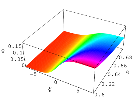
Figure 3: (Color online) Showing how the amplitude and the width of the positive EA-DLs vary with $\beta$ for $\sigma=10$, $\mu=0.5$, and $M=0.38$.

The profiles (indicating height and thickness) of the small amplitude EA-DLs associated with positive potential are graphically displayed in figure 3. It is seen from figure 3 that the amplitude (width) of the EA-DLs decreases (increases) with $\beta$.

V Arbitrary Amplitude EA Solutions

We now investigate the properties of arbitrary amplitude EASPs and EA-DLs by numerical analyses of the pseudo-potential $V(\Psi)$, given by (5). It is evident from (5) that $V(\Psi)=dV(\Psi)/d\Psi=0$ at $\Psi=0$. Therefore, the EASP and EA-DL solutions of (5) exist if $d^{2}V(\Psi)/d\Psi^{2})_{\Psi=0}<0$ i.e., $C_{2}>0$, i.e., $M>M_{c}=\sqrt{(1-\mu)/(\mu+\sigma-\beta\sigma)}$, so that the fixed point at the origin is unstable.

Figure 4: The profile of the pseudo-potential for $\mu=0.5$, $\sigma=10$, $\beta=0.7$, $M=0.4133$ (solid curve), $M=0.41$ (dash curve), and $M=0.415$ (dotted curve).

Figure 5: The profile of the pseudo-potential for $\mu=0.5$, $\sigma=10$, $\beta=0.7$, and $M=0.38$.

One can easily show by numerical analyses of $V(\Psi)$ [given in (5)] that the EASPs exist with both positive potential ($\Psi>0$) and negative potential ($\Psi<0$), but the EA-DLs exist only with positive potential ($\Psi>0$). A part of the numerical analyses, showing the formation of the potential wells in the positive $\Psi$-axis, i.e. showing the existence of the EASPs and EA-DLs with $\Psi>0$, is displayed in Fig. 4. Figure 4 displays the formation of the potential wells in the positive $\Psi$-axis, which corresponds to the formation of the EASPs and EA-DLs with positive potential for $\mu=0.5$, $\sigma=10$, and $\beta=0.7$. The Mach numbers are $0.4133$ (solid curve), corresponding to a double layer solution, $0.41$ (dash curve), yielding a positive solitary solution, $0.415$ (dotted curve), giving no positive solitary structure. Figure 5 exhibits the formation of the potential well in the negative $\Psi$-axis, which corresponds to the formation of EASPs with negative potential for $\mu=0.5$, $\sigma=10$, $\beta=0.7$, and $M=0.38$ (solid curve).

Figure 6: The formation of potential wells in both positive and negative $\Psi$-axes at $\mu=0.3$, $\sigma=10$, $\beta=0.583$, $M=0.41$ (solid curve), and $M=0.411$ (dotted curve).

Figure 7: The formation of potential well in negative $\Psi$-axes at $M=0.95$, $\mu=0.5$, $\sigma=0.4$, and $\beta=0.6$.

Figure 6 exhibits that for $M>M_{c}$ positive and negative EASPs coexist (solid curve), and EA-DLs are formed with positive potential only, but not with negative potential. It also shows that negative EASPs and positive EA-DLs coexist (dotted curve). Figure 7 depicts the formation of the potential well in the negative $\Psi$-axis, which corresponds to the formation of EASPs with negative potential for $\mu=0.5$, $\sigma=0.4$, $\beta=0.6$, and $M=0.95$. Figure 4 can provide a visualization of the amplitude ($\Psi_{m}$) and the width [$|\Psi_{m}|/|V_{m}|$, where $|V_{m}|$ is the minimum value of $V(\Psi)$ in the potential wells formed in the positive $\Psi$ -axis]. Figure 5 can also provide a visualization of the height and the thickness in the potential well formed in the negative $\Psi$ -axis]. Figure 4, where the values of $M$ are around its critical value ($M_{c}$), indicate the existence of arbitrary amplitude EASPs and EA-DLs. Figure 5, where the values of $M$ are around its critical value ($M_{c}$), reveals the existence of arbitrary amplitudes EASPs. It is found from this visualization (after a more numerical analysis with different values of $\mu$, $\sigma$, and $\beta$, which are not shown here) that the variation of the amplitude and the width with $\mu$, $\sigma$, and $\beta$ in the case of arbitrary amplitude EASPs and EA-DLs are exactly the same as that in the case of small amplitude EASPs and EA-DLs.

VI Summary and Conclusions

In this paper, we have considered a plasma composed of cold inertial electrons, hot Boltzmann distributed electrons, and non-isothermal hot ions, and have investigated properties of small but finite, as well as arbitrary amplitudes EASPs and EA-DLs. We have used the pseudo-potential approach, which is valid for arbitrary amplitudes EASPs and EA-DLs. It has been found for the small amplitude limit that (i) the non-thermal plasma system under consideration is found to support EASPs and EA-DLs, whose salient features (the amplitude, the width, the speed, etc.) are significantly modified by the non-thermal parameter $\beta$; (ii) the amplitude (width) of the EASPs decreases (increases) with $\beta$; (iii) the amplitude (width) of the EA-DLs decreases (increases) with $\beta$. On the other hand, it has been found for the arbitrary amplitude that (i) EA-DLs are formed at $M=0.4133$; (ii) positive EASPs are formed at $M=0.41$; (iii) no positive EASPs are formed at $M=0.415$; (iv) the negative EASPs are formed at $M=0.38$; (v) at $M>M_{c}$ the negative EASPs and positive EASPs or EA-DLs coexist; (vi) when ion temperature is greater than hot ion temperature i.e. $\sigma=0.4$ then we get only negative EASPs.

The ranges of different plasma parameters used in our investigation are very wide ($\mu=0.2-0.9$, $\sigma=0.4-10$, and $\beta=0.3-0.8$), are relevant to both space Dubouloz1991 ; Dubouloz1993 ; Pottelette1999 ; Berthomier2000 ; Singh2001 and laboratory plasmas Derfler1969 ; Henry1972 . Thus, the results of the present investigation should help us to explain salient features of localized EA perturbations propagating in space and laboratory plasmas that have two distinct groups of electrons and a component of non-isothermal hot ions.

- (1) B. D. Fried and and R. W. Gould, Phys. Fluids 4, 139 (1961).
- (2) K. Watanabe and T. Taniuti, J. Phys. Soc. Jpn. 43, 1819 (1977).
- (3) S.P. Gary and R. L. Tokar, Phys. Fluids 28, 2439 (1985).
- (4) M. Yu and P. K. Shukla, J. Plasma Phys. 29, 409 (1983).
- (5) R. L. Mace and M. A. Hellberg, J. Plasma Phys. 43, 239 (1990).
- (6) R. L. Mace and M. A. Hellberg, J. Geophys. Res. 98, 5881 (1993).
- (7) R. L. Mace and M. A. Hellberg, Phys. Plasmas 8, 2649 (2001).
- (8) R. L. Mace, S. Baboolal, R. Bharuthram, and M. A. Hellberg, J. Plasma Phys. 45, 323 (1991).
- (9) H. Derfler and T. C. Simonen, Phys. Fluids 12, 269 (1969).
- (10) D. Henry and J. P. Treguier, J. Plasma Phys. 8, 311 (1972).
- (11) T. E. Sheridan, M. J. Goeckner, and J. Goree, J. Vac. Sci. Technol. A 9, 688 (1991).
- (12) J. S. Pickett et al., Adv. Space Res. 41, 1666 (2008).
- (13) A. P. Kakad et al., Adv. Space Res. 43, 1945 (2009).
- (14) C. Moon et al., J. Plasma Fusion Res. SERIES 9, 436 (2010).
- (15) N. Singh and S. Araveti, The Astrophysical J. lett. 733, L6 (2011).
- (16) S. Mondal et al., Proc. Natl. Acad. Sci. 109, 8011 (2012).
- (17) N. Dubouloz, R. Pottelette, M. Malingre, and R. A. Treumann, Geophys. Res. Lett. 18, 155 (1991).
- (18) N. Dubouloz et al., J. Geophys. Res., [Atmos.] 98, 17415 (1993).
- (19) R. Pottelette et al., Geophys. Res. Lett. 26, 2629 (1999).
- (20) M. Berthomier et al., Phys. Plasmas 7, 2987 (2000).
- (21) S. V. Singh and G. S. Lakhina, Planet. Space Sci. 49, 107 (2001).
- (22) R. L. Tokar and S. P. Gary, Geophys. Res. Lett. 11, 1180 (1984).
- (23) D. Schriver and M. Ashour-Abdalla, Geophys. Res. Lett. 16, 899 (1989).
- (24) C. S. Lin et al., J. Geophys. Res. 89, 925 (1984).
- (25) E. K. El-Shewy, Chaos, Solitons & Fractrals 31, 1020 (2007).
- (26) B. Sahu, Phys. Plasmas 17, 122305 (2010).
- (27) M. Dutta et al., Phys. Plasmas 18, 102301 (2011).
- (28) S. A. El-Wakil et al., Phys. Plasmas 18, 092116 (2011).
- (29) G. S. Lakhina et al., Phys. Plasmas 15, 062903 (2008).
- (30) R. A. Cairns et al., Geophys. Res. Lett. 22, 2709 (1995).
- (31) A. A. Mamun, R. A. Cairns, and P. K. Shukla, Phys. Plasmas 3, 2610 (1996).
- (32) A. A. Mamun and P. K. Shukla, Phys. Scripta T98, 107 (2002).
- (33) Y. Futaana et al., J. Geophys. Res. 108, 1025 (2003).
- (34) J. R. Asbridge, S. J. Bame, and I. B. Strong, J. Geophys. Res. 73, 5777 (1968).
- (35) S. Imada, H. Hara, and T. Watanabe, The Astrophysical J. 705, L208 (2009).
- (36) I. B. Bernstein, G. M. Grence, and M. D. Kruskal, Phys. Rev. 108, 546 (1957).
- (37) R. Z. Sagdeev, in Reviews of Plasma Physics, edited by Leontovich, M. A. (Consultants Bureau, New York, 1966), vol. 4, p. 23.
- (38) A. Mannan and A. A. Mamun, Phys. Rev. E 84, 026408 (2011).
- (39) A. A. Mamun and A. Mannan, JETP Lett. 94, 356 (2011).