Adaptive construction of surrogates for the Bayesian solution of inverse problems

Abstract

The Bayesian approach to inverse problems typically relies on posterior sampling approaches, such as Markov chain Monte Carlo, for which the generation of each sample requires one or more evaluations of the parameter-to-observable map or forward model. When these evaluations are computationally intensive, approximations of the forward model are essential to accelerating sample-based inference. Yet the construction of globally accurate approximations for nonlinear forward models can be computationally prohibitive and in fact unnecessary, as the posterior distribution typically concentrates on a small fraction of the support of the prior distribution. We present a new approach that uses stochastic optimization to construct polynomial approximations over a sequence of measures adaptively determined from the data, eventually concentrating on the posterior distribution. The approach yields substantial gains in efficiency and accuracy over prior-based surrogates, as demonstrated via application to inverse problems in partial differential equations.

1 Introduction

In many science and engineering problems, parameters of interest cannot be observed directly; instead, they must be estimated from indirect observations. In these situations, one can usually appeal to a forward model mapping the parameters of interest to some quantities that can be measured. The corresponding inverse problem then involves inferring the unknown parameters from a set of observations [15].

Inverse problems arise in a host of applications, ranging from the geosciences [43, 33, 28, 13] to chemical kinetics [34] and far beyond. In these applications, data are inevitably noisy and often limited in number. The Bayesian approach to inverse problems [22, 42, 43, 47] provides a foundation for inference from noisy and incomplete data, a natural mechanism for incorporating physical constraints and heterogeneous sources of information, and a quantitative assessment of uncertainty in the inverse solution. Indeed, the Bayesian approach casts the inverse solution as a posterior probability distribution over the model parameters or inputs. Though conceptually straightforward, this setting presents challenges in practice. The posterior distributions are typically not of analytical form or from a standard parametric family; characterizing them exactly requires sampling approaches such as Markov chain Monte Carlo [7, 10, 44, 8]. These methods entail repeated solutions of the forward model. When the forward model is computationally intensive, e.g., specified by partial differential equations (PDEs), a direct approach to Bayesian inference becomes computationally prohibitive.

One way to accelerate inference is to construct computationally inexpensive approximations of the forward model and to use these approximations as surrogates in the sampling procedure. Many approximation methods have been successfully employed in this context, ranging from projection-based model reduction [48, 35, 17] to Gaussian process regression [49, 24] to parametric regression [4]. Our previous work [29, 30, 31] has developed surrogate models by using stochastic spectral methods [18, 50] to propagate prior uncertainty from the inversion parameters to the forward model outputs. The result is a forward model approximation that converges in the prior-weighted $L^{2}$ sense. Theoretical analysis shows that if the forward model approximation converges at certain rate in this prior-weighted norm, then (under certain assumptions) the posterior distribution generated by the approximation converges to the true posterior at the same rate [42, 31, 1]. Constructing a sufficiently accurate surrogate model over the support of the prior distribution, however, may not be possible in many practical problems. When the dimension of the parameters is large and the forward model is highly nonlinear, constructing such a “globally accurate” surrogate can in fact be a formidable task.

The inverse problem fortunately has more structure than the prior-based uncertainty propagation problem. Since the posterior distribution reflects some information gain relative to the prior distribution, it often concentrates on a much smaller portion of the parameter space. In this paper, we will propose that: (i) it can therefore be more efficient to construct a surrogate that only maintains high accuracy in the regions of appreciable posterior measure; and (ii) this “localized” surrogate can enable accurate posterior sampling and accurate computation of posterior expectations.

A natural question to ask, then, is how to build a surrogate in the important region of the posterior distribution before actually characterizing the posterior? Inspired by the cross-entropy (CE) method [14, 40] for rare event simulation, we propose an adaptive algorithm to find a distribution that is “close” to the posterior in the sense of Kullback-Leibler divergence and to build a local surrogate with respect to this approximating distribution. Candidate distributions are chosen from a simple parameterized family, and the algorithm minimizes the Kullback-Leibler divergence of the candidate distribution from the posterior using a sequence of intermediate steps, where the optimization in each step is accelerated through the use of locally-constructed surrogates. We demonstrate with numerical examples that the total computational cost of our method is much lower than the cost of building a globally accurate surrogate of comparable or even lesser accuracy. Moreover, we show that the final approximating distribution can provide an excellent proposal for Markov chain Monte Carlo sampling, in some cases exceeding the performance of adaptive random-walk samplers. This aspect of our methodology has links to previous work in adaptive independence samplers [23].

The remainder of this article is organized as follows. In Section 2 we briefly review the Bayesian formulation of inverse problems and previous work using polynomial chaos surrogates to accelerate inference. In Section 3, we present our new adaptive method for the construction of local surrogates, with a detailed discussion of the algorithm and an analysis of its convergence properties. Section 4 provides several numerical demonstrations, and Section 5 concludes with further discussion and suggestions for future work.

2 Bayesian inference and polynomial chaos surrogates

Let $\mathbf{y}\in{\mathbb{R}}^{n_{y}}$ be the vector of parameters of interest and $\mathbf{d}\in{\mathbb{R}}^{n_{d}}$ be a vector of observed data. In the Bayesian formulation, prior information about $\mathbf{y}$ is encoded in the prior probability density $\pi(\mathbf{y})$ and related to the posterior probability density $\pi(\mathbf{y}|\mathbf{d})$ through Bayes’ rule:

$$\pi(\mathbf{y}|\mathbf{d})=\frac{\pi(\mathbf{d}|\mathbf{y})\pi(\mathbf{y})}{\int\pi(\mathbf{d}|\mathbf{y})\pi(\mathbf{y})d\mathbf{y}\,},$$ (1)

where $\pi(\mathbf{d}|\mathbf{y})$ is the likelihood function. (In what follows, we will restrict our attention to finite-dimensional parameters $\mathbf{y}$ and assume that all random variables have densities with respect to Lebesgue measure.) The likelihood function incorporates both the data and the forward model. In the context of an inverse problem, the likelihood usually results from some combination of a deterministic forward model $\mathbf{G}:{\mathbb{R}}^{n_{y}}\rightarrow{\mathbb{R}}^{n_{d}}$ and a statistical model for the measurement noise and model error. For example, assuming additive measurement noise ${\bm{\epsilon}}$, we have

$$\mathbf{d}=\mathbf{G}(\mathbf{y})+{\bm{\epsilon}}\,.$$ (2)

If the probability density of ${\bm{\epsilon}}$ is given by $\pi_{\epsilon}({\bm{\epsilon}})$, then the likelihood function becomes

$$\pi(\mathbf{d}|\mathbf{y})=\pi_{\epsilon}(\mathbf{d}-\mathbf{G}(\mathbf{y}))\ .$$ (3)

For conciseness, we define $\pi^{*}(\mathbf{y}):=\pi(\mathbf{y}|\mathbf{d})$ and $L(\mathbf{G}):=\pi_{\epsilon}(\mathbf{d}-\mathbf{G})$ and rewrite Bayes’ rule (1) as

$$\pi^{*}(\mathbf{y})=\frac{L(\mathbf{G}(\mathbf{y}))\pi(\mathbf{y})}{I},$$ (4)

where

$$I:=\int L(\mathbf{G}(\mathbf{y}))\pi(\mathbf{y})d\mathbf{y}\,$$ (5)

is the posterior normalizing constant or evidence. In practice, no closed form analytical expression for $\pi^{*}(\mathbf{y})$ exists, and any posterior moments or expectations must be estimated via sampling methods such as Markov chain Monte Carlo (MCMC), which require many evaluations of the forward model.

If the forward model has a smooth dependence on its input parameters $\mathbf{y}$, then using stochastic spectral methods to accelerate this computation is relatively straightforward. As described in [29, 30, 31, 16], the essential idea behind existing methods is to construct a stochastic forward problem whose solution approximates the deterministic forward model $\mathbf{G}(\mathbf{y})$ over the support of the prior $\pi(\mathbf{y})$. More precisely, we seek a polynomial approximation $\widetilde{\mathbf{G}}_{N}(\mathbf{y})$ that converges to $\mathbf{G}(\mathbf{y})$ in the prior-weighted $L^{2}$ norm. Informally, this procedure “propagates” prior uncertainty through the forward model and yields a computationally inexpensive surrogate that can replace $\mathbf{G}(\mathbf{y})$ in, e.g., MCMC simulations.

For simplicity, we assume prior independence of the input parameters, namely,

$$\pi(\mathbf{y})=\prod_{j=1}^{n_{y}}\pi_{j}(y_{j})\,.$$

(This assumption can be loosened when necessary; see, for example, discussions in [3, 41].) Since $\mathbf{G}(\mathbf{y})$ is multi-dimensional, we construct a polynomial chaos (PC) expansion for each component of the model output. Suppose that $g(\mathbf{y})$ is a component of $\mathbf{G}(\mathbf{y})$; then its $N$-th order PC expansion is

$$g_{N}(\mathbf{y})=\sum_{|\mathbf{i}|\leq N}a_{\mathbf{i}}\Psi_{\mathbf{i}}(\mathbf{y}),$$ (6)

where $\mathbf{i}:=\left(i_{1},i_{2},\ldots,i_{n_{y}}\right)$ is a multi-index with $|\mathbf{i}|:=i_{1}+i_{2}+\ldots+i_{n_{y}}$, $a_{\mathbf{i}}$ are the expansion coefficients, and $\Psi_{\mathbf{i}}$ are orthogonal polynomial basis functions, defined as

$$\Psi_{\mathbf{i}}(\mathbf{y})=\prod_{j=1}^{n_{y}}\psi_{i_{j}}(y_{j})\,.$$ (7)

Here $\psi_{i_{j}}(y_{j})$ is the univariate polynomial of degree $i_{j}$, from a system satisfying orthogonality with respect to $\pi_{j}$:

$${\mathbb{E}}_{j}\left[\psi_{i}\psi_{i^{\prime}}\right]=\int\psi_{i}\left(y_{j}\right)\psi_{i^{\prime}}\left(y_{j}\right)\pi_{j}\left(y_{j}\right)\,dy_{j}=\delta_{i,i^{\prime}},$$ (8)

where we assume that the polynomials have been properly normalized. It follows that $\Psi_{\mathbf{i}}(\mathbf{y})$ are $n_{y}$-variate orthonormal polynomials satisfying

$${\mathbb{E}}\left[\Psi_{\mathbf{i}}(\mathbf{y})\Psi_{\mathbf{i}^{\prime}}(\mathbf{y})\right]=\int\Psi_{\mathbf{i}}\left(\mathbf{y}\right)\Psi_{\mathbf{i}^{\prime}}\left(\mathbf{y}\right)\pi(\mathbf{y})\,d\mathbf{y}=\delta_{\mathbf{i},\mathbf{i}^{\prime}}\,,$$ (9)

where $\delta_{\mathbf{i},\mathbf{i}^{\prime}}=\prod_{j=1}^{n_{y}}\delta_{i_{j},i^{\prime}_{j}}$.

Because of the orthogonality condition (8), the distribution over which we are constructing the polynomial approximation—namely each prior distribution $\pi_{j}(y_{j})$—determines the polynomial type. For example, Hermite polynomials are associated with the Gaussian distribution, Jacobi polynomials with the beta distribution, and Laguerre polynomials with the gamma distribution. For a detailed discussion of these correspondences and their resulting computational efficiencies, see [51]. For PC expansions corresponding to non-standard distributions, see [46, 2]. Note also that in the equations above, we have restricted our attention to total-order polynomial expansions, i.e., $|\mathbf{i}|\leq N$. This choice is merely for simplicity of exposition; in practice, one may choose any admissible multi-index set $\mathcal{J}\ni\mathbf{i}$ to define the polynomial chaos expansion in (6).

The key computational task in constructing these polynomial approximations is the evaluation of the expansion coefficients $\mathbf{a}_{\mathbf{i}}$. Broadly speaking, there are two classes of methods for doing this: intrusive (e.g., stochastic Galerkin) and non-intrusive (e.g., interpolation or pseudospectral approximation). In this paper, we will follow [31] and use a non-intrusive method to compute the coefficients. The main advantage of a non-intrusive approach is that it only requires a finite number of deterministic simulations of the forward model, rather than a reformulation of the underlying equations. Using the orthogonality relation (9), the expansion coefficients are given by

$$a_{\mathbf{i}}={\mathbb{E}}[g(\mathbf{y})\Psi_{\mathbf{i}}(\mathbf{y})\,],$$ (10)

and thus $a_{\mathbf{i}}$ can be estimated by numerical quadrature

$$\tilde{a}_{\mathbf{i}}=\sum_{m=1}^{M}g(\mathbf{y}^{(m)})\,\Psi_{\mathbf{i}}(\mathbf{y}^{(m)})\,w^{(m)},$$ (11)

where $\mathbf{y}^{(m)}$ are a set of quadrature nodes and $w^{(m)}$ are the associated weights for $m=1,\ldots,M$. Tensor product quadrature rules are a natural choice, but for $n_{y}\geq 2$, using sparse quadrature rules to select the model evaluation points can be vastly more efficient. Care must be taken to avoid significant aliasing errors when using sparse quadrature directly in (11), however. Indeed, it is advantageous to recast the approximation as a Smolyak sum of constituent full-tensor polynomial approximations, each associated with a tensor-product quadrature rule that is appropriate to its polynomials [12]. This type of approximation may be constructed adaptively, thus taking advantage of weak coupling and anisotropy in the dependence of $\mathbf{G}$ on $\mathbf{y}$. More details can be found in [11].

3 Adaptive surrogate construction

The polynomial chaos surrogates described in the previous section are constructed to ensure accuracy with respect to the prior; that is, they converge to the true forward model $\mathbf{G}(\mathbf{y})$ in the $L^{2}_{\pi}$ sense, where $\pi$ is the prior density on $\mathbf{y}$. In many inference problems, however, the posterior is concentrated in a very small portion of the entire prior support. In this situation, it can be much more efficient to build surrogates only over the important region of the posterior. (Consider, for example, a forward model output that varies nonlinearly with $\mathbf{y}$ over the support of the prior. Focusing onto a much smaller range of $\mathbf{y}$ reduces the degree of nonlinearity; in the extreme case, if the posterior is sufficiently concentrated and the model output is continuous, then even a linear surrogate could be sufficient.) In this section we present a general method for constructing posterior-focused surrogates.

3.1 Minimizing cross entropy

The main idea of our method is to build a polynomial chaos surrogate over a probability distribution that is “close” to the posterior in the sense of Kullback-Leibler (K-L) divergence. Specifically, we seek a distribution with density $p(\mathbf{y})$ that minimizes the K-L divergence from $\pi^{\ast}(\mathbf{y})$ to $p$:

$${\mathcal{D}}_{\mathrm{KL}}(\pi^{\ast}\|\,p)=\int\pi^{\ast}(\mathbf{y})\ln\frac{\pi^{\ast}(\mathbf{y})}{p(\mathbf{y})}\,d\mathbf{y}=\int\pi^{\ast}(\mathbf{y})\ln{\pi^{\ast}(\mathbf{y})}\,d\mathbf{y}-\int\pi^{\ast}(\mathbf{y})\ln{p(\mathbf{y})}\,d\mathbf{y}\,.$$ (12)

Interestingly, one can minimize (12) without exact knowledge of the posterior distribution $\pi^{\ast}(\mathbf{y})$. Since the first integral on the right-hand side of (12) is independent of $p$, minimizing ${\mathcal{D}}_{\mathrm{KL}}(\pi^{\ast}\|\,p)$ is equivalent to maximizing

$$\int\pi^{\ast}(\mathbf{y})\ln{p(\mathbf{y})}\,d\mathbf{y}\,=\int{\frac{L(\mathbf{G}(\mathbf{y}))\pi(\mathbf{y})}{I}\ln p(\mathbf{y})\,d\mathbf{y}}\,.$$

Moreover, since $I$ is a constant (for fixed data), one simply needs to maximize $\int{L(\mathbf{G}(\mathbf{y}))\ln p(\mathbf{y})}\pi(\mathbf{y})\,d\mathbf{y}$.

In practice, one selects the candidate distributions $p$ from a parameterized family $\mathcal{P}_{V}=\{p(\mathbf{y};\mathbf{v})\}_{\mathbf{v}\in V}$, where $\mathbf{v}$ is a vector of parameters (called “reference parameters” in the cross-entropy method for rare event simulation) and $V$ is the corresponding parameter space. Thus the desired distribution can be found by solving the optimization problem

$$\max_{\mathbf{v}\in V}D(\mathbf{v})=\max_{\mathbf{v}\in V}\int{L(\mathbf{G}(\mathbf{y}))\ln p(\mathbf{y};\mathbf{v})\pi(\mathbf{y})}\,d\mathbf{y}\,.$$ (13)

3.2 Adaptive algorithm

In this section, we propose an adaptive algorithm to solve the optimization problem above. The algorithm has three main ingredients: sequential importance sampling, a tempering procedure, and localized surrogate models. In particular, we construct a sequence of intermediate optimization problems that converge to the original one in (13), guided by a tempering parameter. In each intermediate problem, we evaluate the objective using importance sampling and we build a local surrogate to replace expensive evaluations of the likelihood function.

We begin by recalling the essentials of importance sampling [39]. Importance sampling (IS) simulates from a biasing distribution that may be different than the original distribution or the true distribution of interest, but corrects for this mismatch by weighing the samples with an appropriate ratio of densities. By focusing samples on regions where an integrand is large, for example, IS can reduce the variance of a Monte Carlo estimator of an integral [25]. In the context of (13), a naïve Monte Carlo estimator might sample from the prior $\pi$, but this estimator will typically have extremely high variance: when the likelihood function is large only on a small fraction of the prior samples, most of the terms in the resulting Monte Carlo sum will be near zero. Instead, we sample from a biasing distribution $q(\mathbf{y})$ and thus rewrite $D$ as:

$$D(\mathbf{v})=\int{L(\mathbf{G}(\mathbf{y}))\ln p(\mathbf{y};\mathbf{v})\frac{\pi(\mathbf{y})}{q(\mathbf{y})}\,q(\mathbf{y})}\,d\mathbf{y}\,,$$ (14a)

and obtain an unbiased IS estimator of $$D$$:

$$\hat{D}(\mathbf{v}):=\frac{1}{M}\sum_{m=1}^{M}{L\left(\mathbf{G}(\mathbf{y}^{(m)})\right)\,l(\mathbf{y}^{(m)}})\,\ln p(\mathbf{y}^{(m)};\mathbf{v}),$$ (14b)

where $l(\mathbf{y}):=\pi(\mathbf{y})/q(\mathbf{y})$ is the density ratio or weight function and the samples $\{\mathbf{y}^{(m)}\}$ in (14b) are drawn independently from $q(\mathbf{y})$.

Next we introduce a tempering parameter $\lambda$, putting

$$L(\mathbf{y};\lambda):=[L(\mathbf{y})]^{\frac{1}{\lambda}},$$

and defining $\pi^{\ast}(\mathbf{y};\lambda)$ as the posterior density associated with the tempered likelihood $L(\mathbf{y};\lambda)$. Here $L(\mathbf{y};\lambda)$ and $\pi^{\ast}(\mathbf{y};\lambda)$ revert to the original likelihood function and posterior density, respectively, for $\lambda=1$. The algorithm detailed below will ensure that $\lambda=1$ is reached within a finite number of steps.

The essential idea of the algorithm is to construct a sequence of biasing distributions $\left(p(\mathbf{y};\mathbf{v}_{k})\right)$, where each $p$ is drawn from the parameterized family $\mathcal{P}$. Each biasing distribution has two roles: first, to promote variance reduction via importance sampling; and second, to serve as the input distribution for constructing a local surrogate model $\widetilde{\mathbf{G}}_{k}(\mathbf{y})$. The final biasing distribution, found by solving the optimization problem when $\lambda=1$, is the sought-after “best approximation” to the posterior described above.

Algorithm 1 Adaptive algorithm

• Input: probability fraction $\rho\in(0,1)$, likelihood function level $\gamma>0$, minimum step size $\delta>0$; initial biasing distribution parameters $\mathbf{v}_{0}$, IS sample size $M$

• Initialize: $k=0$, $\lambda_{0}=\infty$

• while $\lambda_{k}>1$ do

• Construct $\widetilde{\mathbf{G}}_{k}(\mathbf{y})$, the polynomial chaos approximation of $\mathbf{G}_{k}(\mathbf{y})$ with respect to $p(\mathbf{y};\mathbf{v}_{k})$

• Draw $M$ samples $\{\mathbf{y}^{(1)}$, …, $\mathbf{y}^{(M)}\}$ according to $p(\mathbf{y};\mathbf{v}_{k})$.

• Compute $\lambda_{k+1}$ such that the largest $100\rho\%$ percent of the resulting likelihood function values $\{L(\widetilde{\mathbf{G}}_{k}(\mathbf{y}^{(m)};\lambda_{k+1}))\}_{m=1}^{M}$ are larger than $\gamma$.

• if $\lambda_{k+1}>\lambda_{k}-\delta$ then

• $\lambda_{k+1}\leftarrow\lambda_{k}-\delta$

• end if

• if $\lambda_{k+1}<1$ then

• $\lambda_{k+1}\leftarrow 1$

• end if

• Solve the optimization problem:

  $$\mathbf{v}_{k+1}=\arg\max_{\mathbf{v}\in V}\hat{D}_{k+1}(\mathbf{v})=\arg\max_{\mathbf{\mathbf{v}}\in V}\frac{1}{M}\sum^{M}_{n=1}{L(\widetilde{\mathbf{G}}_{k}(\mathbf{y}^{(m)});\lambda_{k+1})\,\ln p(\mathbf{y}^{(m)};\mathbf{v})\,l_{k}(\mathbf{y}^{(m)})}$$

  where $l_{k}(\mathbf{y}):=\pi(\mathbf{y})/p(\mathbf{y};\mathbf{v}_{k})$.

• $k\leftarrow k+1$

• end while

Steps of the algorithm are detailed in Algorithm 1. The basic idea behind the iterations is the following: since $p(\mathbf{y};\mathbf{v}_{k})$, the biasing distribution obtained at step $k$, is close to $\pi^{\ast}(\mathbf{y};\lambda_{k})$, then in the next step, if one can choose $\lambda_{k+1}$ such that $\pi^{\ast}(\mathbf{y};\mathbf{v}_{k})$ and $\pi^{\ast}(\mathbf{y};\mathbf{v}_{k+1})$ are close, the forward model surrogate and the IS estimator based on $p(\mathbf{y};\mathbf{v}_{k})$ should be effective for the optimization problem at step $k+1$. A more formal discussion of the convergence properties of the algorithm is given in Section 3.3. Note that for reasons of computational efficiency, we want the distributions over which we construct the surrogates to remain relatively localized. Thus a good choice for $\mathbf{v}_{0}$ would keep the variance of $p(\mathbf{y};\mathbf{v}_{0})$ relatively small and perhaps center it at the prior mean. The value of $\lambda$ will automatically adjust to the choice of initial biasing distribution.

An important part of the algorithm is the choice of a parameterized family of distributions $\mathcal{P}_{V}$. The distributions should be flexible yet easy to sample, and straightforward to use as an input distribution for the construction of polynomial surrogates. To this end, multivariate normal distributions are a convenient choice. Not only do they suggest the use of the well-studied Gauss-Hermite polynomial chaos expansion for the forward model, but they also make it possible to solve the optimization problem in step 13: of Algorithm 1 analytically. For example, let $p(\mathbf{y};\mathbf{v})$ be an uncorrelated multivariate Gaussian:

$$p(\mathbf{y};\mathbf{v})=\prod_{j=1}^{n_{y}}p_{j}(y_{j})\,,\qquad p_{j}(y_{j})=\frac{1}{\sqrt{2\pi}\sigma_{j}}\exp\left(-\frac{(y_{j}-\mu_{j})^{2}}{2\sigma_{j}^{2}}\right)\,,$$ (15)

where the reference parameters are now $\mathbf{v}=(\mu_{1},\ldots,\mu_{n_{y}},\sigma_{1},\ldots,\sigma_{n_{y}})$. Assuming that $\hat{D}$ in step 13: of Algorithm 1 is convex and differentiable with respect to $\mathbf{v}$, we obtain the solution to $\max_{\mathbf{v}}\hat{D}$ by solving

$$\nabla_{\mathbf{v}}\hat{D}=0\,.$$ (16)

Substituting (15) into (16) yields:

$$\frac{\partial\hat{D}}{\partial{\mu_{j}}}=\frac{1}{M}\sum^{M}_{m=1}{L(\widetilde{\mathbf{G}}_{k}(\mathbf{y}^{(m)}))\,l_{k}(\mathbf{y}^{(m)})\,(2y^{(m)}_{j}-2\mu_{j})}=0\,,$$ (17a)

$$\frac{\partial\hat{D}}{\partial{\sigma_{j}}}=\frac{1}{M}\sum^{M}_{m=1}L(\widetilde{\mathbf{G}}_{k}(\mathbf{y}^{(m)}))\,l_{k}(\mathbf{y}^{(m)})\left(\frac{(y^{(m)}_{j}-\mu_{j})^{2}}{\sigma^{3}_{j}}-\frac{1}{\sigma_{j}}\right)=0\,,$$ (17b)

for $j=1\ldots n_{y}$, the solution of which can readily be found as:

$$\mu_{j}=\frac{\sum^{M}_{m=1}L(\widetilde{\mathbf{G}}_{k}(\mathbf{y}^{(m)}))l_{k}(\mathbf{y}^{(m)})y^{(m)}_{j}}{\sum^{M}_{m=1}L(\widetilde{\mathbf{G}}_{k}(\mathbf{y}^{(m)}))l_{k}(\mathbf{y}^{(m)})}\,,$$ (18a)

$${\sigma_{j}}=\sqrt{\frac{\sum^{M}_{m=1}L(\widetilde{\mathbf{G}}_{k}(\mathbf{y}^{(m)}))l_{k}(\mathbf{y}^{(m)})(y^{(m)}_{j}-\mu_{j})^{2}}{\sum^{M}_{m=1}L(\widetilde{\mathbf{G}}_{k}(\mathbf{y}^{(m)}))l_{k}(\mathbf{y}^{(m)})}}\,.$$ (18b)

This is just an example, of course. We emphasize that our method does not require any specific type of biasing distribution, and that one can freely choose the family $\mathcal{P}_{V}$ that is believed to contain the best approximations of the posterior distribution.

3.3 Convergence analysis

By design, the tempering parameter $\lambda$ in Algorithm 1 reaches 1 in a finite number of steps, and as a result the algorithm converges to the original optimization problem. Thus we only need to analyze the convergence of each step. Without causing any ambiguity, we will drop the step index $k$ throughout this subsection.

First, we set up some notation. Let $\widetilde{\mathbf{G}}_{N}(\mathbf{y})$ be the $N$-th order polynomial chaos approximation of $\mathbf{G}(\mathbf{y})$, based on a biasing distribution $q(\mathbf{y})$. Also, let

$$D_{N}(\mathbf{v}):=\int{L(\widetilde{\mathbf{G}}_{N}(\mathbf{y}))\ln p(\mathbf{y};\mathbf{v})\,l(\mathbf{y})\,q(\mathbf{y})}\,d\mathbf{y}\,,\\$$ (19)

and

$$\hat{D}_{N}(\mathbf{v}):=\frac{1}{M}\sum_{m=1}^{M}{L\left(\widetilde{\mathbf{G}}_{N}(\mathbf{y}^{(m)})\right)\ln p(\mathbf{y}^{(m)};\mathbf{v})\,l(\mathbf{y}^{(m)}})\,,$$ (20)

where $l(\mathbf{y}):=\pi(\mathbf{y})/q(\mathbf{y})$, and $\mathbf{y}^{(m)}$ are sampled independently from $q(\mathbf{y})$. Note that, for any $\mathbf{v}$, $\hat{D}_{N}$ is a random variable but $D_{N}$ is a deterministic quantity. We make the following assumptions:

Assumption 1.

1. The biasing distribution $q(\mathbf{y})$ satisfies

   $$\|\ln(p(\mathbf{y};\mathbf{v}))l(\mathbf{y})\|_{L^{2}_{q}}<\infty,$$ (21)

   where $\|\cdot\|_{L^{2}_{q}}$ is the $L^{2}$-norm with weight $q(\mathbf{y})$;

2. The likelihood function $L(\mathbf{g})$ is bounded and uniformly continuous (with respect to $\mathbf{g}$) on $\{\mathbf{g}=\mathbf{G}(\mathbf{y}):q(\mathbf{y})>0\}\cup\{\mathbf{g}=\widetilde{\mathbf{G}}_{N}(\mathbf{y}):q(\mathbf{y})>0,\ N\geq 1\}$.

Now we give a lemma that will be used to prove our convergence results:

Lemma 2.

Suppose that Assumption 1(a) holds. If

$$\lim_{N\rightarrow\infty}\|\widetilde{\mathbf{G}}_{N}(\mathbf{y})-\mathbf{G}(\mathbf{y})\|_{L^{2}_{q}}=0,$$

then

$$\lim_{N\rightarrow\infty}\|L(\widetilde{\mathbf{G}}_{N}(\mathbf{y}))-L(\mathbf{G}(\mathbf{y}))\|_{L^{2}_{q}}=0.$$

Proof.

See Appendix. ∎

Our main convergence result is formalized in the proposition below.

Proposition 3.

Suppose that Assumption 1 holds. Then we have

$$\lim_{M,\,N\rightarrow\infty}\|\hat{D}_{N}(\mathbf{v})-D(\mathbf{v})\|_{L^{2}_{q}}=0.$$ (22)

Proof.

The variance of estimator (20) is

$$\|\hat{D}_{N}(\mathbf{v})-D_{N}(\mathbf{v})\|^{2}_{L^{2}_{q}} = \frac{1}{M}\left(\|L(\widetilde{\mathbf{G}}_{N}(\mathbf{y}))\ln p(\mathbf{y};\mathbf{v})\,l(\mathbf{y})\|^{2}_{L^{2}_{q}}-D_{N}^{2}\right)$$ (23)

$$\leq \frac{1}{M}\left(C\|\ln p(\mathbf{y};\mathbf{v})\,l(\mathbf{y})\|^{2}_{L^{2}_{q}}-D_{N}^{2}\right),$$

where $C>0$ is some constant, and it follows immediately that

$$\lim_{M\rightarrow\infty}\|\hat{D}_{N}(\mathbf{v})-D_{N}(\mathbf{v})\|_{L^{2}_{q}}=0.$$ (24)

We then look at the truncation error between $D_{N}(\mathbf{v})$ and $D(\mathbf{v})$:

$$|D_{N}(\mathbf{v})-D(\mathbf{v})| = \left|\int{(L(\widetilde{\mathbf{G}}_{N}(\mathbf{y}))-L(\mathbf{G}(\mathbf{y})))\ln p(\mathbf{y};\mathbf{v})\,l(\mathbf{y})q(\mathbf{y})}\,d\mathbf{y}\right|$$ (25)

$$\leq \left\|(L(\widetilde{\mathbf{G}}_{N}(\mathbf{y}))-L(\mathbf{G}(\mathbf{y})))\ln p(\mathbf{y};\mathbf{v})\,l(\mathbf{y})q(\mathbf{y})\right\|_{L^{1}_{q}}$$

$$\leq \|{L(\widetilde{\mathbf{G}}_{N}(\mathbf{y}))}-{L(\mathbf{G}(\mathbf{y}))}\|_{L^{2}_{q}}\,\left\|\ln p(\mathbf{y};\mathbf{v})\,l(\mathbf{y})\right\|_{L^{2}_{q}},$$

by Hölder’s inequality. Using Lemma 2 and (21), one obtains

$$\lim_{N\rightarrow\infty}|D_{N}(\mathbf{v})-D(\mathbf{v})|=0,$$ (26)

which together with (24) implies that $\hat{D}_{N}(\mathbf{v})\rightarrow D(\mathbf{v})$ in $L^{2}_{q}$, as $M,\,N\rightarrow\infty$. ∎

We note that the analysis above is not limited to total-order polynomial chaos expansions; it is applicable to other polynomial chaos truncations and indeed to other approximation schemes. What is required are the conditions of Lemma 2, where $N$ is any parameter that indexes the accuracy of the forward model approximation, such that $\lim_{N\rightarrow\infty}\|\widetilde{\mathbf{G}}_{N}(\mathbf{y})-\mathbf{G}(\mathbf{y})\|_{L^{2}_{q}}=0$.

3.4 Independence sampler MCMC

In addition to providing a surrogate model focused on the posterior distribution, the adaptive algorithm also makes it possible to employ a Metropolis-Hastings independence sampler, i.e., an MCMC scheme where the proposal distribution is independent of the present state [44] of the Markov chain. When the proposal distribution is close to the posterior, the independence sampler can be much more efficient than a standard random walk Metropolis-Hastings scheme [19, 32, 37], in that it enables larger “jumps” across the parameter space. This suggests that the final biasing distribution $p(\mathbf{y};\mathbf{v})$ found by our method can be a good proposal distribution for use in MCMC simulation.

Let the final biasing distribution obtained by Algorithm 1 be denoted by $p(\mathbf{y};\mathbf{v}_{\infty})$, and let the corresponding surrogate model be $\widetilde{\mathbf{G}}_{\infty}(\mathbf{y})$. In each MCMC iteration, the independence sampler updates the current state $\mathbf{y}_{t}$ of the Markov chain via the following steps:

1. Propose a candidate state $\mathbf{y}^{\prime}$ by drawing a sample from $p(\mathbf{y};\mathbf{v}_{\infty})$.

2. Compute the Metropolis acceptance ratio:

   $$\alpha=\frac{L(\widetilde{\mathbf{G}}_{\infty}(\mathbf{y}^{\prime}))\,\pi(\mathbf{y}^{\prime})}{L(\widetilde{\mathbf{G}}_{\infty}(\mathbf{y}_{t}))\,\pi(\mathbf{y}_{t})}\frac{p(\mathbf{y}_{t};\mathbf{v}_{\infty})}{p(\mathbf{y}^{\prime};\mathbf{v}_{\infty})}\,.$$ (27)

3. Put $r=\max(\alpha,1)$. Draw a number $r^{\prime}\sim U(0,1)$ and set the next state of the chain to:

   $$\mathbf{y}_{t+1}=\left\{\begin{array}[]{cc}\mathbf{y}^{\prime},&r^{\prime}\leq r;\\ \mathbf{y}_{t},&r^{\prime}>r.\end{array}\right.$$

Given the final surrogate $\widetilde{\mathbf{G}}_{\infty}(\mathbf{y})$, one could also use a standard random-walk MCMC sampler, or any other valid MCMC algorithm, to explore the posterior induced by this forward model approximation. A comparison of the Metropolis independence sampler with an adaptive random-walk MCMC approach will be provided in Section 4.2.

4 Numerical examples

In this section we present two numerical examples to explore the efficiency and accuracy of the adaptive surrogate construction method. The first example is deliberately chosen to be low-dimensional for illustration purposes. The second is a classic time-dependent inverse heat conduction problem.

4.1 Source inversion

First we will apply our method to the contaminant source inversion problem studied in [30], which uses a limited and noisy set of observations to infer the location of a contaminant source. Specifically, we consider a dimensionless diffusion equation on a two-dimensional spatial domain:

$$\frac{\partial u}{\partial{t}}=\nabla^{2}u+s(\mathbf{x},t),\qquad\mathbf{x}\in D:=[0,1]^{2},$$ (29)

with source term $s(\mathbf{x},t)$. The field $u(\mathbf{x},t)$ represents the concentration of a contaminant. The source term describes the release of the contaminant at spatial location $\mathbf{x}_{\mathrm{src}}:=(x_{1},x_{2})$ over the time interval $[0,\tau]$:

$$s(\mathbf{x},t)=\left\{\begin{array}[]{cc}\frac{s}{2\pi h^{2}}\exp\left(-{|\mathbf{x}_{\mathrm{src}}-\mathbf{x}|^{2}}/{2h^{2}}\right),&0\leq t\leq\tau\\ 0,&t>\tau\end{array}\right.$$ (32)

Here we suppose that the source strength $s$ is known and equal to 2.0, the source width $h$ is known and equal to 0.05, and the source location $\mathbf{x}_{\mathrm{src}}$ is the parameter of interest. The contaminant is transported by diffusion but cannot leave the domain; we thus impose homogeneous Neumann boundary conditions:

$$\nabla u\cdot\mathbf{n}=0\ \ \mathrm{on}\ \partial D.$$

At the initial time, the contaminant concentration is zero everywhere:

$$u\left(\mathbf{x},0\right)=0.$$

The diffusivity is spatially uniform; with a suitable scaling of space/time, we can always take its value to be unity.

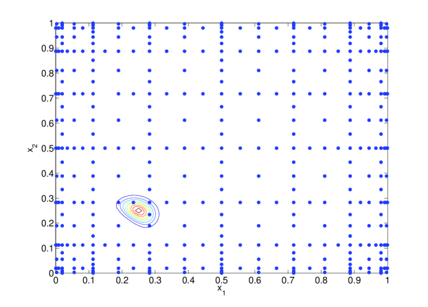
(a) Prior-based surrogate.

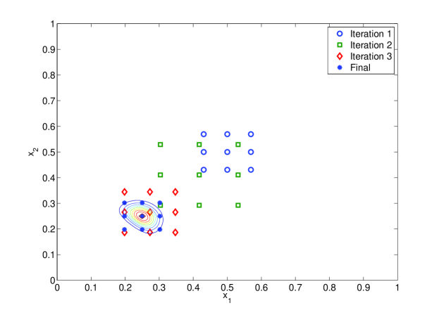
(b) Adaptive surrogate.

Fig. 1: Source inversion problem: model evaluation points used to construct the prior-based and adaptive surrogates. In the bottom figure (adaptive method), the circles, squares, and diamonds are the points evaluated in the first, second, and third iterations, respectively. Contours of the posterior probability density are superimposed on each figure.

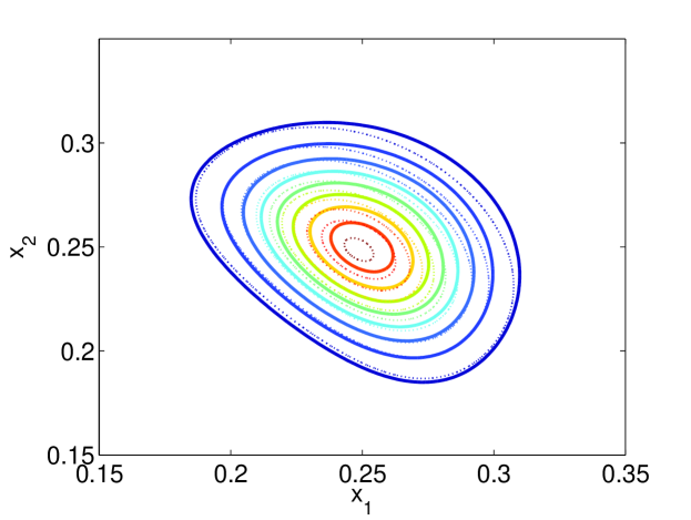
(a) “True” posterior density (solid line), compared with the posterior density obtained via the prior-based surrogate (dotted line).

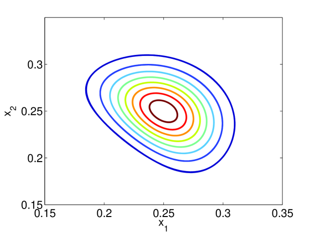
(b) “True” posterior density (solid line), compared with the posterior density obtained via the adaptively-constructed surrogate (dashed line).

Fig. 2: Source inversion problem: posterior density of $\mathbf{x}_{\mathrm{src}}$ obtained with the three different approaches. In the bottom figure, the two sets of contours are virtually indistinguishable.

Sensors that measure local concentration values are placed on a uniform $3\times 3$ grid covering $D$, and sensor readings are provided at two successive times, $t=0.1$ and $t=0.2$, resulting in a total of 18 measurements. The forward model thus maps the source position to the values of the field $u(\mathbf{x},t)$ at the prescribed measurement locations and times, while the inverse problem consists of inferring the source position from noisy measurements. We write the forward model as $\mathbf{d}=\mathbf{G}(\mathbf{x}_{\mathrm{src}})+{\bm{\epsilon}}$, where $\mathbf{d}$ is the vector collecting all the measurements and ${\bm{\epsilon}}$ is the measurement error. Each component of ${\bm{\epsilon}}$ is assumed to be an independent zero-mean Gaussian random variable: $\epsilon_{i}\sim N(0,\sigma^{2})$ with $\sigma=0.1$ for $i=1\ldots 18$. In this example we generate simulated data $\mathbf{d}$ by solving the forward model with $\mathbf{x}_{\mathrm{src}}=(0.25,\,0.25)$ and adding noise. To complete the Bayesian setup, we take the prior to be a uniform distribution over $D$; that is, $x_{j}\sim U(0,1)$ for $j=1,\,2$.

First we characterize the posterior distribution using the proposed adaptive method. We fix the polynomial order of the surrogates $\widetilde{\mathbf{G}}_{k}(x_{1},x_{2})$ to $N=4$ and take the biasing distribution to be an uncorrelated Gaussian:

$$p(x_{1},x_{2};\mathbf{v})=\frac{1}{2\pi\sigma_{1}\sigma_{2}}\exp\left(-\frac{(x_{1}-\mu_{1})^{2}}{2\sigma_{1}^{2}}-\frac{(x_{2}-\mu_{2})^{2}}{2\sigma_{2}^{2}}\right)\,,$$ (33)

where the means $\mu_{1}$, $\mu_{2}$ and standard deviations $\sigma_{1}$, $\sigma_{2}$ comprise the reference parameters $\mathbf{v}$. The initial biasing distribution is centered at the prior mean and has small variance; that is, we choose $\mu_{1}=\mu_{2}=0.5$ and $\sigma_{1}=\sigma_{2}=0.05$. We set $\rho=0.05$, $\gamma=10^{-3}$, and put $\delta=(\lambda_{0}-1)/10$ (namely, we require $\lambda$ to reach $1$ in at most 10 iterations). In each iteration, a $3\times 3$ tensor product Gaussian-Hermite quadrature rule is used to construct a Hermite polynomial chaos surrogate, resulting in nine true model evaluations; $M=5\times 10^{4}$ surrogate samples are then employed to estimate the reference parameters. It takes four iterations for the algorithm to converge, and its main computational cost thus consists of evaluating the true model 36 times.

As a comparison, we also construct a polynomial surrogate with respect to the uniform prior distribution. Here we use a surrogate composed of total order $N=9$ Legendre polynomials, and compute the polynomial coefficients with a level-6 sparse grid based on Clenshaw-Curtis quadrature, resulting in 417 true model evaluations—about 12 times as many as the adaptive method. These values were chosen so that the prior-based and adaptive polynomial surrogates have comparable (though not exactly equal) accuracy.

In Figure 1, we show the points in parameter space at which the true model was evaluated in order to construct the two types of surrogates. Contours of the posterior density are superimposed on the points. It is apparent that in the prior-based method, although 417 model evaluation points are used, only five of them actually fall in the region of significant posterior probability. With the adaptive method, on the other hand, 8 of the 36 model evaluations occur in the important region of the posterior distribution. Figure 2 shows the posterior probability densities resulting from both types of surrogates. Since the problem is two-dimensional, these contours were obtained simply by evaluating the posterior density on a fine grid, thus removing any potential MCMC sampling error from the problem. Also shown in the figure is the posterior density obtained with direct evaluations of the true forward model, i.e., the “true” posterior. While both surrogates provide reasonably accurate posterior approximations, the adaptive method is clearly better; its posterior is essentially identical to the true posterior. Moreover, the adaptive method requires an order of magnitude fewer model evaluations than the prior-based surrogate.

4.2 Inverse heat conduction

Estimating temperature or heat flux on an inaccessible boundary from the temperature history measured inside a solid gives rise to an inverse heat conduction (IHC) problem. These problems have been studied for several decades due to their significance in a variety of scientific and engineering applications [6, 36, 48, 26]. An IHC problem becomes nonlinear if the thermal properties are temperature-dependent [5, 9]; this feature renders inversion significantly more difficult than in the linear case. In this example we consider a one-dimensional heat conduction equation:

$$\frac{\partial u}{\partial{t}}=\frac{\partial}{\partial{x}}\left[c(u)\frac{\partial u}{\partial{x}}\right],$$ (34)

where $x$ and $t$ are the spatial and temporal variables, $u(x,t)$ is the temperature, and

$$c(u):=\frac{1}{1+u^{2}}$$

is the temperature-dependent thermal conductivity, all in dimensionless form. The equation is subject to initial condition $u(x,0)=u_{0}(x)$ and Neumann boundary conditions:

$$\frac{\partial}{\partial{x}}u(0,t)=q(t),$$ (35a)

$$\frac{\partial}{\partial{x}}u(L,t)=0,$$ (35b)

where $L$ is the length of the medium. In other words, one end ($x=L$) of the domain is insulated and the other ($x=0$) is subject to heat flux $q(t)$. Now suppose that we place a temperature sensor at $x=x_{s}$. The goal of the IHC problem is to infer the heat flux $q(t)$ for $t\in[0,\,T]$ from the temperature history measured at the sensor over the same time interval. A schematic of this problem is shown in Figure 3.

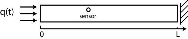
Fig. 3: Schematic of the one-dimensional heat conduction problem.

For the present simulations, we put $L=1$ and $T=1$ and let the initial condition be $u_{0}(x)=0$. We parameterize the flux signal with a Fourier series:

$$q(t)=a_{0}+\sum_{j=1}^{N_{f}}\left(a_{j}\cos(2j\pi t/T)+b_{j}\sin(2j\pi t/T)\right),\qquad 0\leq t\leq T,$$ (36)

where $a_{j}$ and $b_{j}$ are the coefficients of the cosine and sine components, respectively, and $N_{f}$ is the total number of Fourier modes. In the following tests, we will fix $N_{f}=4$; the inverse problem is thus 9-dimensional. The sensor is placed at $x_{s}=0.4$, the temperature is measured at 50 regularly spaced times over the time interval $[0,T]$, and the error in each measurement is assumed to be an independent zero-mean Gaussian random variable with variance $\sigma^{2}=10^{-2}$.

To generate data for inversion, the “true” flux is chosen to be

$$q_{\mathrm{true}}(t)=\sum_{j=1}^{4}(1.5\cos(2j\pi t)+1.5\sin(2j\pi t))\,,$$ (37)

i.e., $a_{0}=0$, $a_{j}=1.5$, and $b_{j}=1.5$ for $j=1\ldots 4$. Figure 4(a) shows the entire solution of (34) with the prescribed “true” flux, with the sensor location indicated by the dashed line. The inverse problem becomes more ill-posed as the sensor moves to the right, away from the boundary where $q$ is imposed; information about the time-varying input flux is progressively destroyed by the nonlinear diffusion. Figure 4(b) makes this fact more explicit, by showing the temperature history at $x=0$ (i.e., the boundary subject to the heat flux) and at $x=0.4$ (where the sensor is placed). The data for inversion are generated by perturbing the latter profile with the i.i.d. observational noise. A finer numerical discretization of (34) is used to generate these data than is used in the inference process. To complete the Bayesian setup, we endow the Fourier coefficients with independent Gaussian priors that have mean zero and variance $2$.

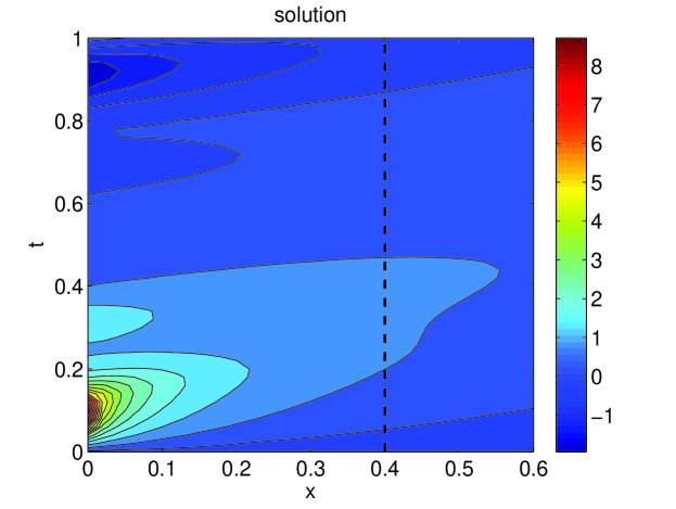
(a) Solution of the nonlinear diffusion equation (34) as a function of space and time. The dashed line indicates the location of the sensor.

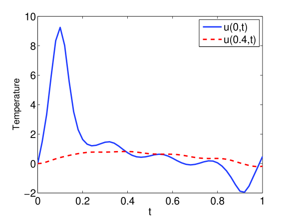
(b) Temperature history at $x=0$ (the boundary where the time-dependent heat flux $q(t)$ is imposed, solid line); and at $x=0.4$ (location of the sensor, dashed line).

Fig. 4: Forward solution of the transient heat conduction problem.

	number of	${\mathcal{D}}_{\mathrm{KL}}(\pi^{\ast}\|\,\pi_{\mathrm{PC}})$	${\mathcal{D}}_{\mathrm{KL}}(\pi^{\ast}\|\,\pi_{\mathrm{PC}})$
surrogate	model evaluations	$\pi(a_{1},b_{1})$	$\pi(a_{4},b_{4})$
prior-based
$N=3,S=6$	11833	124	1.89
prior-based
$\bm{N=5,\,S=7}$	35929	8.37	0.383
adaptive
$N=2,S=3$	$2445$	0.0044	0.0129
adaptive
$\bm{N=2,\,S=5}$	$4459$	0.0032	0.0127

Table 1: Cost and performance comparison of prior-based and adaptively-constructed surrogates.

We now use the adaptive algorithm to construct a localized polynomial chaos surrogate, and compare its computational cost and performance to that of a prior-based surrogate. In both cases, we use Hermite polynomial chaos to approximate the forward model, and sparse grids based on tensorization of univariate delayed Kronrod-Patterson rules [38] to compute the polynomial coefficients (non-intrusively). To test the prior-based method, we use two different total-order truncations of the PC expansion, one at $N=3$ (with sparse grid level $S=6$) and the other at $N=5$ (with sparse grid level $S=7$). Sparse grid levels were chosen to ensure relatively small aliasing error in both cases.

To run the adaptive algorithm, we set $\rho=0.05$, $\gamma=10^{-3}$, and $\delta=(\lambda_{0}-1)/20$ (see Algorithm 1) and we use $M=10^{5}$ samples for importance sampling at each step. The initial biasing distribution is centered at the prior mean, with the variance of each component set to $0.5$. As described in (15), the biasing distributions are chosen simply to be uncorrelated Gaussians. The optimization procedure takes 14 iterations to converge, and at each iteration, a new surrogate with $N=2$ and $S=3$ is constructed with respect to the current biasing distribution. Once the final biasing distribution is obtained, we construct a corresponding final surrogate of the same polynomial order, $N=2$. Here we typically employ the same sparse grid level as in the adaptive iterations, but we also report results for a higher sparse grid level ($S=5$) just to ensure that aliasing errors are small. The total number of full model evaluations associated with the adaptive procedure, contrasted with the number used to construct the prior-based surrogates, is shown in the second column of Table 1.

With various final surrogates $\widetilde{\mathbf{G}}$ in hand (both prior-based and adaptively constructed), we now replace the exact likelihood function $L(\mathbf{G})$ with $L(\widetilde{\mathbf{G}})$ to generate a corresponding collection of posterior distributions for comparison. We use a delayed-rejection adaptive Metropolis (DRAM) MCMC algorithm [20] to draw $5\times 10^{5}$ samples from each distribution, and discard the first $10^{4}$ samples as burn-in. To examine the results, we cannot visualize the 9-dimensional posteriors directly; instead we consider several ways of extracting posterior information from the samples.

First, we focus on the Fourier coefficients directly. Figure 5 shows kernel density estimates [21] of the marginal posterior densities of Fourier coefficients of the heat flux $q(t)$. Figure 5(a) shows coefficients of the lowest frequency modes, while Figure 5(b) shows coefficients of the highest-frequency modes. In each figure, we show the posterior densities obtained by evaluation of the exact forward forward model, evaluation of the adaptive surrogate, and evaluation of the prior-based surrogate. The latter two surrogates correspond to the second and fourth rows of Table 1 (marked in bold type). Even though construction of the prior-based surrogate employs more than 6 times as many model evaluations as the adaptive algorithm, the adaptive surrogate is far more accurate. This assessment is made quantitative by evaluating the K-L divergence from the exact posterior distribution to each surrogate-induced posterior distribution (focusing only on the two-dimensional marginals). Results are shown in the last two columns of Table 1. By this measure, the adaptive surrogate is three orders of magnitude more accurate in the low-frequency modes and at least an order of magnitude more accurate in the high-frequency modes. (Here the K-L divergences have also been computed from the kernel density estimates of the pairwise posterior marginals. Sampling error in the K-L divergence estimates is limited to the last reported digit.) The difference in accuracy gains between the low- and high-frequency modes may be due to the fact that the posterior concentrates more strongly for the low-frequency coefficients, as these are the modes for which the data/likelihood are most informative. Thus, while the adaptive surrogate here provides higher accuracy in all the Fourier modes, improvement over the prior surrogate is expected to be most pronounced in the directions where posterior concentration is greatest.

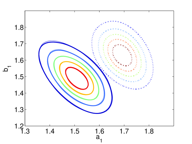
(a) $\pi^{\ast}(a_{1},b_{1}).$

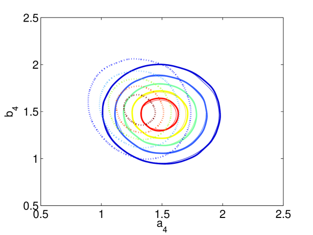
(b) $\pi^{\ast}(a_{4},b_{4}).$

Fig. 5: Inverse heat conduction problem: marginal posterior densities of pairs of Fourier coefficients. Solid lines (thicker) are results of the exact forward model; solid lines (thinner) are from the adaptive surrogate; dotted lines are from the prior-based surrogate.

To further assess the performance of the adaptive method, we use posterior samples of the Fourier coefficients to reconstruct posterior moments of the heat flux itself, again using the exact forward model, the adaptively-constructed surrogate, and the prior surrogate. Figure 6 shows the posterior mean, Figure 6 shows the posterior variance, and Figure 8 shows the posterior skewness; these are moments of the marginal posterior distributions of heat flux $q(t)$ at any given time $t$. Again, we show results only for the surrogates identified in the second and fourth lines of Table 1. The adaptively-constructed (and posterior-focused) surrogate clearly outperforms the prior-based surrogate. Note that the nonzero skewness is a clear indicator of the non-Gaussian character of the posterior.

Moving from moments of the marginal distributions to correlations between heat flux values at different times, Figure 9 shows the posterior autocovariance of the heat flux computed with the adaptive surrogate, which also agrees well with the values computed from the true model.

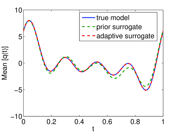
Fig. 6: Inverse heat conduction problem: posterior mean of the flux $q(t)$ computed with the true model, the prior-based surrogate, and the adaptively-constructed surrogate.

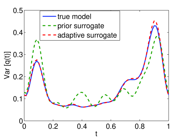
Fig. 7: Inverse heat conduction problem: posterior variance of the flux $q(t)$ computed with the true model, the prior-based surrogate, and the adaptively-constructed surrogate.

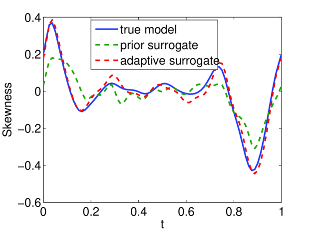
Fig. 8: Inverse heat conduction problem: posterior skewness of the flux $q(t)$ computed with the true model, the prior-based surrogate, and the adaptively-constructed surrogate.

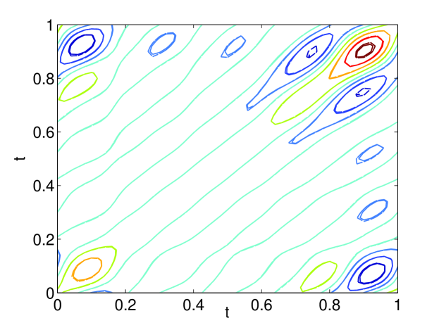
Fig. 9: Inverse heat conduction problem: posterior covariance of the flux $q(t)$. Solid lines are computed from the exact-model posterior, while dashed lines are computed with the adaptive surrogate.

Finally, we evaluate the MCMC independence sampler proposed in Section 3.4, comparing its performance with that of the adaptive random-walk sampler (DRAM). For the present inverse heat conduction problem, the mixing of each sampler is essentially independent of the particular posterior (exact or surrogate-based) to which it is applied; we therefore report results for the adaptive surrogate only. Figure 10 plots the empirical autocorrelation of the MCMC chain as a function of lag, computed from $5\times 10^{5}$ iterations of each sampler. We focus on the MCMC chain of $a_{1}$, but the relative autocorrelations of other Fourier coefficients are similar. Rapid decay of the autocorrelation is indicative of good mixing; MCMC iterates are less correlated, and the variance of any MCMC estimate at a given number of iterations is reduced. Figure 10 shows that autocorrelation decays considerably faster with the independence sampler than with the random-walk sampler, which suggests that the final biasing distribution computed with the adaptive algorithm can indeed be a good proposal distribution for MCMC.

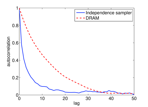
Fig. 10: Chain autocorrelation of an MCMC independence sampler derived from the adaptive algorithm, versus an adaptive random-walk MCMC sampler.

5 Conclusions

This paper has developed an efficient adaptive approach for approximating computationally intensive forward models for use in Bayesian inference. These approximations are used as surrogates for the exact forward model or parameter-to-observable map, thus making sampling-based Bayesian solutions to the inverse problem more computationally tractable.

The present approach is adaptive in the sense that it uses the data and likelihood function to focus the accuracy of the forward model approximation on regions of high posterior probability. This focusing is performed via an iterative procedure that relies on stochastic optimization. In typical inference problems, where the posterior concentrates on a small fraction of the support of the prior distribution, the adaptive approach can lead to significant gains in efficiency and accuracy over previous methods. Numerical demonstrations on inference problems involving partial differential equations show order-of-magnitude increases in computational efficiency (as measured by the number of forward solves) and accuracy (as measured by posterior moments and information divergence from the exact posterior) over prior-based surrogates employing comparable approximation schemes.

The adaptive algorithm generates a finite sequence of biasing distributions from a chosen parametric family, and accelerates the identification of these biasing distributions by constructing approximations of the forward model at each step. The final biasing distribution in this sequence minimizes Kullback-Leibler divergence from the true posterior; convergence to this minimizer is assured as the number of samples (in an internal importance sampling estimator) goes to infinity and the accuracy of the local surrogate is increased. As a byproduct of the algorithm, the final biasing distribution can also serve as a useful proposal distribution for Markov chain Monte Carlo exploration of the posterior distribution.

Since the adaptive approach relies on concentration of the posterior relative to the prior, it is best suited for inference problems where the data are informative in the same relative sense. Yet most “useful” inference problems will fall into this category. The more difficult it is to construct a globally accurate surrogate (for instance, as the forward model becomes more nonlinear) and the more tightly the posterior concentrates, the more beneficial the adaptive approach may be. Now in an ill-posed inverse problem, the posterior may concentrate in some directions but not in others; for instance, data in the inverse heat conduction problem are less informative about higher frequency variations in the inversion parameters. Yet significant concentration does occur overall, and it is largest in the directions where the likelihood function varies most and is thus most difficult to approximate. This correspondence is precisely to the advantage of the adaptive method.

We note that the current algorithm does not require access to derivatives of the forward model. If derivatives were available and the posterior mode could be found efficiently, then it would be natural to use a Laplace approximation at the mode to initialize the adaptive procedure. Also, an expectation-maximization (EM) algorithm could be an interesting alternative to the adaptive importance sampling approach used to solve the optimization problem in (13). Localized surrogate models could be employed to accelerate computations within an EM approach, just as they are used in the present importance sampling algorithm.

Finally, we emphasize that while the current numerical demonstrations used polynomial chaos approximations and Gaussian biasing distributions, the algorithm presented here is quite general. Future work could explore other families of biasing distributions and other types of forward model approximations—even projection-based model reduction schemes. Simple parametric biasing distributions could also be replaced with finite mixtures (e.g., Gaussian mixtures), with a forward model approximation scheme tied to the components of the mixture. Another useful extension of the adaptive algorithm could involve using full model evaluations from previous iterations to reduce the cost of constructing the local surrogate at the current step.

Appendix A Proof of Lemma 2

We start with $L(\mathbf{G})$ being uniformly continuous, which means that for any $\epsilon>0$, there exists a $\delta>0$ such that, for any $|\mathbf{G}_{N}-\mathbf{G}|<\delta$, one has $|L(\mathbf{G}_{N})-L(\mathbf{G})|<\sqrt{\epsilon/2}$. On the other hand, $\mathbf{G}_{N}(\mathbf{y})\rightarrow\mathbf{G}(\mathbf{y})$ in $L^{2}_{q}$ as $N\rightarrow\infty$, implying that $\mathbf{G}_{N}(\mathbf{y})\rightarrow\mathbf{G}(\mathbf{y})$ in probability as $N\rightarrow\infty$; therefore, for the given $\epsilon$ and $\delta$, there exists a positive integer $N_{o}$ such that, for all $N>N_{o}$, ${\mathbb{P}}[|\mathbf{G}_{N}(\mathbf{y})-\mathbf{G}(\mathbf{y})|>\delta]<\epsilon/4$. Let $\Omega:=\{\mathbf{z}:|\mathbf{G}_{N}(\mathbf{y})-\mathbf{G}(\mathbf{y})|<\delta\}$ and let ${\Omega^{\ast}}$ be the complement of $\Omega$ in the support of $q$. Then we can write

$$\|L(\mathbf{G}_{N}(\mathbf{y}))-L(\mathbf{G}(\mathbf{y}))\|^{2}_{L^{2}_{q}}\\ =\int_{\Omega}(L(\mathbf{G}_{N}(\mathbf{y}))-L(\mathbf{G}(\mathbf{y})))^{2}q(\mathbf{y})d\mathbf{y}+\int_{{\Omega^{\ast}}}(L(\mathbf{G}_{N}(\mathbf{y}))-L(\mathbf{G}(\mathbf{y})))^{2}q(\mathbf{y})d\mathbf{y}$$ (38)

The first integral on the right hand side of (38) is smaller than $\epsilon/2$ by design. Now recall that the likelihood function $L(\cdot)$ is bounded, and without loss of generality we assume $0<L(\cdot)<1$. It then follows that the second integral on the right-hand side of (38) is smaller than $\epsilon/2$ too. Thus we complete the proof. $\square$

References

- [1] D. Lucor A. Birolleau, G. Poëtte, Adaptive Bayesian inference for discontinuous inverse problems: application to hyperbolic conservation laws, preprint, (2013).
- [2] M. Arnst, R. Ghanem, E. Phipps, and J. Red-Horse, Measure transformation and efficient quadrature in reduced-dimensional stochastic modeling of coupled problems, International Journal for Numerical Methods in Engineering, 92 (2012), pp. 1044–1080.
- [3] Ivo Babuska, Fabio Nobile, and Raul Tempone, A stochastic collocation method for elliptic partial differential equations with random input data, SIAM Review, 52 (2010), pp. 317–355.
- [4] S. Balakrishnan, A. Roy, M.G. Ierapetritou, G.P. Flach, and P.G. Georgopoulos, Uncertainty reduction and characterization for complex environmental fate and transport models: An empirical Bayesian framework incorporating the stochastic response surface method, Water Resources Research, 39 (2003), p. 1350.
- [5] J.V. Beck, Nonlinear estimation applied to the nonlinear inverse heat conduction problem, International Journal of heat and mass transfer, 13 (1970), pp. 703–716.
- [6] J.V. Beck, CR St Clair, and B. Blackwell, Inverse heat conduction: Ill-posed problems, John Wiley and Sons Inc., New York, NY, 1985.
- [7] J. Besag, P. Green, D. Higdon, and K. Mengersen, Bayesian computation and stochastic systems, Statistical Science, 10 (1995), pp. 3–66.
- [8] S. Brooks, A. Gelman, G. L. Jones, and X.-L. Meng, eds., Handbook of Markov Chain Monte Carlo, Chapman & Hall/CRC, 2011.
- [9] A. Carasso, Determining surface temperatures from interior observations, SIAM Journal on Applied Mathematics, 42 (1982), pp. 558–574.
- [10] M. H. Chen, Q. M. Shao, and J. G. Ibrahim, Monte Carlo methods in Bayesian computation, Springer Verlag, 2000.
- [11] P. Conrad and Y. Marzouk, Adaptive Smolyak pseudospectral approximation, SIAM Journal on Scientific Computing, (2012). submitted.
- [12] P. G. Constantine, M. S. Eldred, and E. T. Phipps, Sparse Pseudospectral Approximation Method, Computer Methods in Applied Mechanics and Engineering, 229–232 (2012), pp. 1–12.
- [13] T Cui, C Fox, and MJ O’Sullivan, Bayesian calibration of a large-scale geothermal reservoir model by a new adaptive delayed acceptance metropolis hastings algorithm, Water Resources Research, 47 (2011).
- [14] P.T. De Boer, D.P. Kroese, S. Mannor, and R.Y. Rubinstein, A tutorial on the cross-entropy method, Annals of Operations Research, 134 (2005), pp. 19–67.
- [15] S. N. Evans and P. B. Stark, Inverse problems as statistics, Inverse Problems, 18 (2002), pp. R55–R97.
- [16] M. Frangos, Y. Marzouk, K. Willcox, and B. van Bloemen Waanders, Surrogate and reduced-order modeling: a comparison of approaches for large-scale statistical inverse problems, in Computational Methods for Large-Scale Inverse Problems and Quantification of Uncertainty, L. Biegler, G. Biros, O. Ghattas, M. Heinkenschloss, D. Keyes, B. Mallick, Y. Marzouk, L. Tenorio, B. van Bloemen Waanders, and K. Willcox, eds., Wiley, 2010.
- [17] D. Galbally, K. Fidkowski, K. Willcox, and O. Ghattas, Nonlinear model reduction for uncertainty quantification in large-scale inverse problems, International Journal for Numerical Methods in Engineering, 81 (2010), pp. 1581–1608.
- [18] R. G. Ghanem and P.D. Spanos, Stochastic finite elements: a spectral approach, Dover, 2003.
- [19] W.R. Gilks, S. Richardson, and D.J. Spiegelhalter, Markov chain Monte Carlo in practice, Chapman & Hall/CRC, 1996.
- [20] H. Haario, M. Laine, A. Mira, and Eero Saksman, DRAM: Efficient adaptive MCMC, Statistics and Computing, 16 (2006), pp. 339–354.
- [21] A. Ihler and M. Mandel, Kernel density estimation toolbox for matlab. http://www.ics.uci.edu/ ihler/code/kde.html.
- [22] J.P. Kaipio and E. Somersalo, Statistical and computational inverse problems, Springer, 2005.
- [23] J. Keith, D. Kroese, and G. Sofronov, Adaptive independence samplers, Statistics and Computing, 18 (2008), pp. 409–420.
- [24] M. C. Kennedy and A. O’Hagan, Bayesian calibration of computer models, Journal of the Royal Statistical Society: Series B, 63 (2001), pp. 425–464.
- [25] J. S. Liu, Monte Carlo Strategies in Scientific Computing, Springer Verlag, 2001.
- [26] D. R. Macayeal, J. Firestone, and E. Waddington, Paleothermometry by control methods, Journal of Glaciology, 37 (1991), pp. 326–338.
- [27] D. MacKay, Information Theory, Inference, and Learning Algorithms, Cambridge University Press, 2002.
- [28] A. Malinverno, Parsimonious Bayesian Markov chain Monte Carlo inversion in a nonlinear geophysical problem, Geophysical Journal International, 151 (2002), pp. 675–688.
- [29] Y. M. Marzouk and H. N. Najm, Dimensionality reduction and polynomial chaos acceleration of Bayesian inference in inverse problems, Journal of Computational Physics, 228 (2009), pp. 1862–1902.
- [30] Y. M. Marzouk, H. N. Najm, and L. A. Rahn, Stochastic spectral methods for efficient Bayesian solution of inverse problems, Journal of Computational Physics, 224 (2007), pp. 560–586.
- [31] Y. M. Marzouk and D. Xiu, A stochastic collocation approach to Bayesian inference in inverse problems, Communications in Computational Physics, 6 (2009), pp. 826–847.
- [32] S.P. Meyn, R.L. Tweedie, and P.W. Glynn, Markov chains and stochastic stability, Springer London et al., 1993.
- [33] K. Mosegaard and M. Sambridge, Monte Carlo analysis of inverse problems, Inverse Problems, 18 (2002), pp. R29–R54.
- [34] H. N. Najm, B.J. Debusschere, Y.M. Marzouk, S. Widmer, and O.P. Le Maitre, Uncertainty Quantification in Chemical Systems, Int. J. Num. Meth. Eng., (2008). in review.
- [35] N. C. Nguyen, G. Rozza, D.B.P. Huynh, and A. T. Patera, Reduced basis approximation and a posteriori error estimation for parametrized parabolic PDEs: Application to real-time bayesian parameter estimation, in Computational Methods for Large-Scale Inverse Problems and Quantification of Uncertainty, L. Biegler, G. Biros, O. Ghattas, M. Heinkenschloss, D. Keyes, B. Mallick, Y. Marzouk, L. Tenorio, B. van Bloemen Waanders, and K. Willcox, eds., Wiley, 2010.
- [36] M.N. Özisik and H.R.B. Orlande, Inverse heat transfer: fundamentals and applications, Hemisphere Pub, 2000.
- [37] N. Petra, J. Martin, G. Stadler, and O. Ghattas, A computational framework for infinite-dimensional Bayesian inverse problems: stochastic Newton MCMC with application to ice sheet inverse problems, preprint, (2013).
- [38] K. Petras, Smolyak cubature of given polynomial degree with few nodes for increasing dimension, Numerische Mathematik, 93 (2003), pp. 729–753.
- [39] C. P. Robert and G. Casella, Monte Carlo Statistical Methods, Springer Verlag, 2004.
- [40] R.Y. Rubinstein and D.P. Kroese, The cross-entropy method: a unified approach to combinatorial optimization, Monte-Carlo simulation, and machine learning, Springer-Verlag, New York, 2004.
- [41] Christian Soize and Roger Ghanem, Physical systems with random uncertainties: Chaos representations with arbitrary probability measure, SIAM Journal on Scientific Computing, 26 (2004), pp. 395–410.
- [42] A. M. Stuart, Inverse problems: a Bayesian perspective, Acta Numerica, 19 (2010), pp. 451–559.
- [43] A. Tarantola, Inverse problem theory and methods for model parameter estimation, Society for Industrial Mathematics, 2005.
- [44] L. Tierney, Markov chains for exploring posterior distributions, the Annals of Statistics, 22 (1994), pp. 1701–1728.
- [45] R. Turner, P. Berkes, and M. Sahani, Two problems with variational expectation maximisation for time-series models, in Workshop on Inference and Estimation in Probabilistic Time-Series Models, vol. 2, 2008.
- [46] X. Wan and G. Karniadakis, Multi-element generalized polynomial chaos for arbitrary probability measures, SIAM Journal on Scientific Computing, 28 (2006), pp. 901–928.
- [47] J. Wang and N. Zabaras, Hierarchical Bayesian models for inverse problems in heat conduction, Inverse Problems, 21 (2005), p. 183.
- [48] J. Wang and N. Zabaras, Using Bayesian statistics in the estimation of heat source in radiation, International Journal of Heat and Mass Transfer, 48 (2005), pp. 15–29.
- [49] B. Williams, D. Higdon, J. Gattiker, L. Moore, M. McKay, and S. Keller-McNulty, Combining experimental data and computer simulations, with an application to flyer plate experiments, Bayesian Analysis, 1 (2006), pp. 765–792.
- [50] D. Xiu, Numerical Methods for Stochastic Computations: A Spectral Method Approach, Princeton, 2010.
- [51] D. Xiu and G. Karniadakis, The Wiener-Askey polynomial chaos for stochastic differential equations, SIAM Journal on Scientific Computing, 24 (2002), pp. 619–644.