Chaos Forgets and Remembers:
Measuring Information Creation, Destruction, and Storage

Abstract

The hallmark of deterministic chaos is that it creates information—the rate being given by the Kolmogorov-Sinai metric entropy. Since its introduction half a century ago, the metric entropy has been used as a unitary quantity to measure a system’s intrinsic unpredictability. Here, we show that it naturally decomposes into two structurally meaningful components: A portion of the created information—the ephemeral information—is forgotten and a portion—the bound information—is remembered. The bound information is a new kind of intrinsic computation that differs fundamentally from information creation: it measures the rate of active information storage. We show that it can be directly and accurately calculated via symbolic dynamics, revealing a hitherto unknown richness in how dynamical systems compute.

Keywords: chaos, entropy rate, bound information, Shannon information measures, information diagram, Tent map, Logistic map, Lozi map

The world is replete with systems that generate information—information that is then encoded in a variety of ways: Erratic ant behavior eventually leads to intricate, structured colony nests [1, 2]; thermally fluctuating magnetic spins form complex domain structures [3]; music weaves theme, form, and melody with surprise and innovation [4]. We now appreciate that the underlying dynamics in such systems is frequently deterministic chaos [5, 6]. In others, the underlying dynamics appears to be fundamentally stochastic [7]. For continuous-state systems, at least, one operational distinction between deterministic chaos and stochasticity is found in whether or not information generation diverges with measurement resolution [8]. This result calls back to Kolmogorov’s original use [9] of Shannon’s mathematical theory of communication [10] to measure a system’s rate of information generation in terms of the metric entropy. Since that time, metric entropy has been understood as a unitary quantity. Whether deterministic or stochastic, it is a system’s degree of unpredictability. Here, we show that this is far too simple a picture—one that obscures much.

To ground this claim, consider two systems. The first, a fair coin: Each flip is independent of the others, leading to a simple uncorrelated randomness. As a result, no statistical fluctuation is predictively informative. For the second system consider a stock traded via a financial market: While its price is unpredictable, the direction and magnitude of fluctuations can hint at its future behavior. (This, at least, is the guiding assumption of the now-global financial engineering industry.) We make this distinction rigorous here, dividing a system’s information generation into a component that is relevant to temporal structure and a component divorced from it. We show that the temporal component captures the system’s internal information processing and, therefore, is of practical interest when harnessing the chaotic nature of physical systems to build novel machines and devices [11]. We first introduce the new measures, describe how to interpret and calculate them, and then apply them via a generating partition to analyze several dynamical systems—the Logistic, Tent, and Lozi maps—revealing a previously hidden form of active information storage.

We observe these systems via an optimal measuring instrument—called a generating partition—that encodes all of their behaviors in a stationary process: A distribution $\Pr(\dots,{X}_{-2},{X}_{-1},{X}_{0},{X}_{1},{X}_{2},\ldots)$ over a bi-infinite sequence of random variables with shift-invariant statistics. A contiguous block of observations ${X}_{t:t+\ell}$ begins at index $t$ and extends for length $\ell$. (The index is inclusive on the left and exclusive on the right.) If an index is infinite, we leave it blank. So, a process is compactly denoted $\Pr({X}_{:})$. Our analysis splits ${X}_{:}$ into three segments: the present ${X}_{0}$, a single observation; the past ${X}_{:0}$, everything prior; and future ${X}_{1:}$, everything that follows.

Figure 1: A process’s I-diagram showing how the past ${X}_{:0}$, present ${X}_{0}$, and future ${X}_{1:}$ partition each other into seven distinct information atoms. We focus only on the four regions contained in the present information $\operatorname{H}[{X}_{0}]$ (blue circle). That is, the present decomposes into three components: $\rho_{\mu}$ (horizontal lines), $r_{\mu}$ (vertical lines), and $b_{\mu}$ (diagonal crosshatching). The redundant information $\rho_{\mu}$ overlaps with the past $\operatorname{H}[{X}_{:0}]$; the ephemeral information $r_{\mu}$ falls outside both the past and the future $\operatorname{H}[{X}_{1:}]$. The bound information $b_{\mu}$ is that part of $\operatorname{H}[{X}_{0}]$ which is in the future yet not in the past.

The information-theoretic relationships between these three random variable segments are graphically expressed in a Venn-like diagram, known as an I-diagram [12]; see Fig. 1. The rate $h_{\mu}$ of information generation is the amount of new information in an observation ${X}_{0}$ given all the prior observations ${X}_{:0}$:

$$h_{\mu}=\operatorname{H}[{X}_{0}|{X}_{:0}]~{},$$ (1)

where $\operatorname{H}[Y|Z]$ denotes the Shannon conditional entropy of random variable $Y$ given variable $Z$. This quantity arises in various contexts and goes by many names: e.g., the Shannon entropy rate and the Kolmogorov-Sinai metric entropy, mentioned above [8]. The complement of the entropy rate is the predicted information $\rho_{\mu}$:

$$\rho_{\mu}=\operatorname{I}[{X}_{:0}:{X}_{0}]~{},$$ (2)

where $\operatorname{I}[Y:Z]$ denotes the mutual information between random variables $Y$ and $Z$ [12]. Hence, $\rho_{\mu}$ is the information in the present that can be predicted from prior observations. Together, we have a decomposition of the information contained in the present: $\operatorname{H}[{X}_{0}]=h_{\mu}+\rho_{\mu}$.

A simple application of the entropy chain rule [12] to Eq. (1) leads us to a different view:

$$h_{\mu} =\operatorname{I}[{X}_{0}:{X}_{1:}|{X}_{:0}]+\operatorname{H}[{X}_{0}|{X}_{:0},{X}_{1:}]$$

$$=b_{\mu}+r_{\mu}~{}.$$ (3)

This introduces two new information measures:

$$b_{\mu} =\operatorname{I}[{X}_{0}:{X}_{1:}|{X}_{:0}]\text{~{}and~{}}$$ (4)

$$r_{\mu} =\operatorname{H}[{X}_{0}|{X}_{:0},{X}_{1:}]~{}.$$ (5)

That is, created information ($h_{\mu}$) decomposes into two parts: information ($b_{\mu}$) shared by the present and the future but not in the past and information ($r_{\mu}$) in the present but in neither the past nor the future.

The $r_{\mu}$ component was first studied by Verdú and Weissman [13] as the erasure entropy (their $H^{-}$) to measure information loss in erasure channels. To emphasize that it is information existing only in a single moment—created and then immediately forgotten—we refer to $r_{\mu}$ as the ephemeral information. The second component $b_{\mu}$ we call the bound information since it is information created in the present that the system stores and that goes on to affect the future . It was first studied as a measure of “interestingness” in computational musicology by Abdallah and Plumbley [15]. For a more complete analysis of this decomposition, as well as computation methods and related measures, see Ref. [16].

Isolating the information $\operatorname{H}[{X}_{0}]$ contained in the present and identifying its components provides the partitioning illustrated in Fig. 1. This is a particularly intuitive way of thinking about the information contained in an observation. While, some behavior ($\rho_{\mu}$) can be predicted, the rest ($h_{\mu}=b_{\mu}+r_{\mu}$) cannot. Of that which cannot be predicted, some ($b_{\mu}$) plays a role in the future behavior and some ($r_{\mu}$) does not. As such, this is a natural decomposition of a time series; one that results in a semantic dissection of the entropy rate.

By way of an example, consider a few simple processes and how their present information decomposes into these three components. A periodic process of alternating $0$s and $1$s ($\ldots 01010101\ldots$) has $\operatorname{H}[{X}_{0}]=1$ bit since $0$s and $1$s occur equally often. Given a prior observation, one can accurately predict exactly which symbol will occur next and so $\operatorname{H}[{X}_{0}]=\rho_{\mu}=1$ bit, while $r_{\mu}=b_{\mu}=0$ bits. On the other extreme is a fair coin flip. Again, each outcome is equally likely and so $\operatorname{H}[{X}_{0}]=1$ bit. However, each flip is independent of all others and so $\operatorname{H}[{X}_{0}]=r_{\mu}=1$ bit, while $\rho_{\mu}=b_{\mu}=0$ bits.

Between these two extrema lie interesting processes: those with stochastic structure. Processes expressing a fixed template, like the periodic process above, contain a finite amount of information. Those with stochastic structure, however, constantly generate information and store it in the form of patterns. Being neither purely predictable nor independently random, these patterns are captured by $b_{\mu}$. The more intricate the organization, the larger $b_{\mu}$. More to the point, generating these patterns requires intrinsic computation in a system—information creation, storage, and transformation [17]. We propose $b_{\mu}$ as a simple method of discovering this type of physical computation: Where there are intricate patterns, there is sophisticated processing.

How useful is the proposed decomposition and its measures? To answer this we analyze several discrete-time chaotic dynamical systems—the Logistic and Tent maps of the interval and the Lozi map of the plane—uncovering a number of novel properties embedded in these familiar and oft-studied systems. As an independent calibration for the measures, we employ Pesin’s theorem [18]: $h_{\mu}$ is the sum of the positive Lyapunov characteristic exponents (LCEs). The maps here have at most one positive LCE $\lambda$, so $h_{\mu}=\max\{0,\lambda\}$. The symbols $s_{0},s_{1},s_{2},\ldots,s_{N}$ for each process we analyze come from a generating partition. We produce a long sample of $N\approx 10^{10}$ symbols, extracting subsequence statistics via a sliding window . Each window consists of a past, present, and future symbol sequence and we estimate $r_{\mu}$ and $b_{\mu}$ using truncated forms of Eqs. (4) and (5).

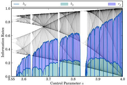
Figure 2: Logistic map information anatomy as a function of control parameter $a$: Bound information $b_{\mu}$ is the lower (green shaded) component; ephemeral information $r_{\mu}$ is the upper (blue shaded) component. Entropy rate is the top (blue) line: $h_{\mu}=b_{\mu}+r_{\mu}$. As reference to the dynamical behavior, the map’s bifurcation diagram is displayed in the background.

Consider first the Logistic map, perhaps one of the most studied chaotic systems:

$$x_{n+1}=ax_{n}(1-x_{n})~{},$$ (6)

where $a\in[0,4]$ is the control parameter and the initial condition is $x_{0}\in[0,1]$. Its generating partition is defined by:

$$s_{n}=\begin{cases}0&\mbox{if }x_{n}<\frac{1}{2}\\ 1&\mbox{if }x_{n}\geq\frac{1}{2}\end{cases}~{}.$$ (7)

Figure 2 shows the resulting measures as a function of control $a$, with the map’s bifurcation diagram displayed in the background for reference.

The first point of interest is that the system’s information generation is, in fact, a mixture of ephemeral ($r_{\mu}$) and bound ($b_{\mu}$) informations at nearly all chaotic ($h_{\mu}>0$) parameter values. The second is that the division into the two components varies in a nontrivial way as a function of the control parameter $a$. Moreover, the boundary between the two appears nondifferentiable. At first blush, this is not surprising given that their sum $h_{\mu}$ ($=\lambda$) is known to be nondifferentiable. Finally, $b_{\mu}$ vanishes nontrivially only at parameters that coincide with the merging of the chaotic bands (e.g., $a=4.0,3.67857\ldots,3.59257\ldots,\ldots$). Thus, the information generated by the Logistic map at these parameters is entirely forgotten.

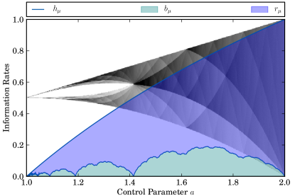
Figure 3: Tent map information anatomy: Although $h_{\mu}=b_{\mu}+r_{\mu}$ is a smooth function of control—$h_{\mu}=\log_{2}a$—the decomposition into bound and ephemeral informations is not. Graphics layout as in previous figure.

Is the complex and nondifferentiable boundary between $r_{\mu}$ and $b_{\mu}$ simply a consequence of the entropy rate’s complicated behavior or due a dynamical mechanism distinct from information creation? We answer this by analyzing the Tent map:

$$x_{n+1}=\frac{a}{2}\left(1-2\left|x_{n}-\frac{1}{2}\right|\right)~{},$$ (8)

where $a\in[0,2]$ is the control parameter. The generating partition for the Tent map is the same as for the Logistic map. Since the Tent map is piecewise linear, its Lyapunov exponent is simply $\lambda=\log_{2}{a}$ and, by Pesin’s theorem, so is the information generation $h_{\mu}=\log_{2}{a}$; a rather smooth parameter dependence. As a result, the intricate structures exhibited in the Tent map’s bifurcation diagram cannot be resolved by studying solely the behavior of the Lyapunov exponent (or $h_{\mu}$) itself. Figure 3 demonstrates that, despite the entropy rate’s simple logarithmic dependence on control, its decomposition $h_{\mu}=b_{\mu}+r_{\mu}$ is not a smooth function of $a$. To emphasize, in sharp contrast with $h_{\mu}$’s simplicity, $r_{\mu}$ and $b_{\mu}$ again appear nondifferentiable—a complexity masked by the smooth $h_{\mu}$. Thus, the two informational components capture a property in the chaotic system’s behavior that is both quantitatively and qualitatively new. As with the Logistic map, we once again find that the bound information vanishes and that all of the information the Tent map generates is forgotten ($h_{\mu}=r_{\mu}$) at parameters corresponding to merging of chaotic bands ($a=2^{1/2^{k}},k=0,1,2,\ldots$). In the Supplementary Materials we show how to calculate $b_{\mu}$ and $r_{\mu}$ in closed form for the Tent map at Misiurewicz parameters.

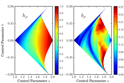
Figure 4: Lozi map information anatomy: (Left) $h_{\mu}$ as a function of controls $a$ and $b$. (Right) $b_{\mu}$ similarly. $b_{\mu}$ is maximized on the upper-right and lower-right edges of the $a$-$b$ region that supports an attractor near the origin.

To explore how these measures apply more generally, we extend information anatomy to two dimensions by analyzing the Lozi map:

$$x_{n+1} =1-a\left|x_{n}\right|+y_{n}$$ (9)

$$y_{n+1} =bx_{n}~{}.$$

The map exhibits an attractor near the origin within a diamond-shaped parameter region inside $(a,b)\in[1,2]\times[-0.9,0.9]$. Note that when $b=0$ the map becomes isomorphic to the Tent map. The generating partition is given by:

$$s_{n}=\begin{cases}0&\mbox{if }x_{n}<0\\ 1&\mbox{if }x_{n}\geq 0\end{cases}~{}.$$ (10)

Figure 4 shows $h_{\mu}$ (left) and $b_{\mu}$ (right) in the attracting parameter region. Mirroring the Tent map, the Lozi map’s entropy rate varies smoothly over the attractor region, whereas $b_{\mu}$ varies in a more complicated manner. There are swaths of low $b_{\mu}$ corresponding to “fuzzy” mergings of chaotic bands. Notably, while the maximal $h_{\mu}$ occurs along the line $b=0$, maximal $b_{\mu}$ occurs far from $b=0$. Hence, large $h_{\mu}$ does not necessarily imply large bound information $b_{\mu}$.

To sum up, we showed that a process’s information creation rate decomposes, via a chain rule, into two structurally meaningful components. The components, the ephemeral information $r_{\mu}$ and the bound information $b_{\mu}$, provide direct insights into a system’s behavior without detailed modeling or appealing to domain-specific knowledge. That is to say, they are relatively easily defined measures that can be straightforwardly estimated. More to the point, however, $b_{\mu}$ is a strong indicator of intrinsic computation. While related to information generation, we demonstrated that it captures a different kind of informational processing—a mechanism that actively stores information.

Concretely, decomposing information creation in the symbolic dynamics of the Logistic, Tent, and Lozi systems delineated the topography of their intrinsic-computation landscape. Awareness of this rich (and previously hidden) landscape will lead to improved engineering of natural systems as substrates for information processing [11]. And, it will lead to an expanded understanding of evolved information processing systems, such as the linguistic processes comprising human natural languages. A sequel will develop the decomposition further, including a geometric interpretation of active information storage that parallels the geometric view of information creation expressed in the Lyapunov exponents.

KB is supported by a UC Davis Chancellor’s Post-Doctoral Fellowship. This work was partially supported by ARO grant W911NF-12-1-0288.

Computing Bound and Ephemeral Informations Analytically

Figure 5: (Above) Tent map’s invariant distribution at parameter $a$ as defined in Eq. (12), consisting of three contiguous, uniformly distributed parts, each differently colored for clarity. (Below) The same colors superimposed on the map itself along with (dotted line) guides to show that the uniform components of the invariant distribution do indeed form a Markov partition.

To obviate the data requirements for accurately estimating $b_{\mu}$ from a time series, we present a method for computing it analytically, in closed form. An analytic expression is possible if one can construct forward-time and reverse-time models of the system. These models are sufficient statistics of the past about the present and future, and the future about the present and past, respectively. Here, we use $\epsilon$-machines [S1, S2], which are the minimal sufficient statistics. From these, $b_{\mu}$ can be computed via:

$$b_{\mu}=\operatorname{I}[{X}_{0}:\mathcal{S}^{+}_{0}|\mathcal{S}^{-}_{1}]~{},$$ (11)

where $\mathcal{S}^{+}_{0}$ is the forward $\epsilon$-machine’s state random variable at time $0$—the minimal sufficient statistic of the past about the present and future—and $\mathcal{S}^{-}_{1}$ is the reverse-time $\epsilon$-machine’s state random variable at time $1$—the minimal sufficient statistic of the future about the present and future. Due to their standing as sufficient statistics, these states stand in for the future ${X}_{1:}$ and the past ${X}_{:0}$ of Eq. (4).

We explicitly implement this calculation for one parameter value of the Tent map. In particular, consider the Misiurewicz point where $f^{4}(\tfrac{1}{2})=f^{5}(\tfrac{1}{2})$. Solving this constraint gives parameter value:

$$a =\alpha+\frac{2}{3\alpha}$$ (12)

$$=1.76929235\ldots$$

where $\alpha=\sqrt[3]{\sqrt{\frac{19}{27}}+1}$. There, the Tent map admits a Markov partition [S3], as Fig. 5 demonstrates. From this, a Markov chain is constructed and the generating partition overlaid. The result is the hidden Markov model of Fig. 6(right) that exactly describes the map’s symbolic dynamics stochastic process.

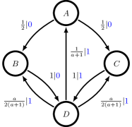
Figure 6: (Left) Markov chain induced by the Markov partition. (Right) The generating partition applied to the transitions, resulting in a hidden Markov model that describes the Tent map’s symbolic stochastic process.

Equation (11) requires the model to be a sufficient statistic to calculate $b_{\mu}$. And so, we transform the hidden Markov model of Fig. 6(right) to one that is unifilar and, in particular, to the $\epsilon$-machine of Fig. 7.

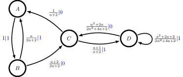
Figure 7: The (unifilar) $\epsilon$-machine for the hidden Markov model of Fig. 6(right). That is, for each state there is at most a single outgoing transition labeled with each symbol. This makes the states a function of the past ${X}_{:0}$ and so allows for the required calculation.

As the final step, we construct the process’s bidirectional machine [S1, S2] from the $\epsilon$-machine; the result is shown in Fig. 8. Then, from it we calculate the joint distribution $\Pr(\mathcal{S}^{+}_{0},\mathcal{S}^{-}_{0},{X}_{0},\mathcal{S}^{+}_{1},\mathcal{S}^{-}_{1})$. This, in turn, allows one to calculate $b_{\mu}=\operatorname{H}[{X}_{0}|\mathcal{S}^{+}_{0},\mathcal{S}^{-}_{1}]$ and $r_{\mu}=\operatorname{I}[{X}_{0}:\mathcal{S}^{-}_{1}|\mathcal{S}^{+}_{0}]$. We find that the Tent map at the Misiurewicz parameter $a$ has the following information measures (in bits per step):

$$h_{\mu} =\log_{2}{a}=\log_{2}\left(\frac{\sqrt[3]{9+\sqrt{57}}+\sqrt[3]{9-\sqrt{57}}}{3^{\frac{2}{3}}}\right)$$

$$=0.823172\ldots$$

$$r_{\mu} =\frac{1}{4}\left(3-\frac{2}{a+1}-\frac{4}{a+2}+\frac{9}{2a+3}\right)$$

$$=\frac{1}{9}\left(\frac{\sqrt[3]{207\sqrt{57}-1349}}{19^{2/3}}-\frac{32}{\sqrt[3]{19\left(207\sqrt{57}-1349\right)}}+7\right)$$

$$=0.648258\ldots$$

$$b_{\mu} =h_{\mu}-r_{\mu}$$

$$=0.174915\ldots~{}.$$

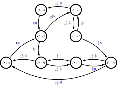
Figure 8: Bidirectional machine of the stochastic process generated by the Tent map’s symbolic dynamics at the Misiurewicz parameter $a$. Its states are pairs $\mathcal{S}^{+}_{0}:\mathcal{S}^{-}_{0}$. By utilizing the dynamic (the edges that connect states), it allows one to directly calculate $\operatorname{H}[{X}_{0}|\mathcal{S}^{+}_{0},\mathcal{S}^{-}_{1}]$ and, thus, $r_{\mu}$ and $b_{\mu}$.

Supplementary References

S1. J. P. Crutchfield, C. J. Ellison, and J. R. Mahoney, “Time’s Barbed Arrow: Irreversibility, Crypticity, and Stored Information”, Phys. Rev. Lett. 103:9 (2009) 094101.

S2. C. J. Ellison, J. R. Mahoney, and J. P. Crutchfield, “Prediction, Retrodiction, and the Amount of Information Stored in the Present”, J. Stat. Phys. 136:6 (2009) 1005–1034.

S3. D. Lind and B. Marcus. An Introduction to Symbolic Dynamics and Coding. Cambridge University Press, 1999.

References

- [1] E. Bonabeau, G. Theraulaz, and M. Dorigo, editors. Swarm Intelligence: From Natural to Artificial Systems. Oxford University Press, New York, 1999.
- [2] S. Camazine, J.-L. Deneubourg, N. R. Franks, J. Sneyd, G. Theraulas, and E. Bonabeau. Self-Organization in Biological Systems. Princeton University Press, New York, 2003.
- [3] J. J. Binney, N. J. Dowrick, A. J. Fisher, and M. E. J. Newman. The Theory of Critical Phenomena. Oxford University Press, Oxford, 1992.
- [4] B. R. Simms. Music of the Twentieth Century: Style and Structure. Schirmer Books, New York, second edition, 1996.
- [5] S. H. Strogatz. Nonlinear Dynamics and Chaos: With Applications to Physics, Biology, Chemistry, and Engineering. Westview Press, 1994.
- [6] J. B. Jose and E. J. Saletan. Classical Dynamics: A Contemporary Approach. Cambridge University Press, New York, 1998.
- [7] R. F. Streater. Statistical Dynamics: A Stochastic Approach to Nonequilibrium Thermodynamics. Imperial College Press, London, second edition, 2009.
- [8] P. Gaspard and X.-J. Wang. Noise, chaos, and (epsilon,tau)-entropy per unit time. Physics Reports, 235(6):291–343, 1993.
- [9] A. N. Kolmogorov. Entropy per unit time as a metric invariant of automorphisms. Dokl. Akad. Nauk. SSSR, 124:754, 1959. (Russian) Math. Rev. vol. 21, no. 2035b.
- [10] C. E. Shannon. A mathematical theory of communication. Bell Sys. Tech. J., 27:379–423, 623–656, 1948.
- [11] W. L. Ditto, A. Miliotis, K. Murali, S. Sinha, and M. L. Spano. Chaogates: Morphing logic gates that exploit dynamical patterns. Chaos, 20(3):037107, 2010.
- [12] R. W. Yeung. Information Theory and Network Coding. Springer, New York, 2008.
- [13] S. Verdú and T. Weissman. The Information Lost in Erasures. IEEE Trans. Info. Th., 54(11):5030–5058, 2008.
- [14] Our terminology avoids the misleading use of the phrase “predictive information” for . The latter is not the amount of information needed to predict the future. Rather, it is part of the predictable information—that portion of the future which can be predicted.
- [15] S. A. Abdallah and M. Plumbley. Information dynamics: Patterns of expectation and surprise in the perception of music. Connection Science, 21(2):89–117, June 2009.
- [16] R. G. James, C. J. Ellison, and J. P. Crutchfield. Anatomy of a Bit: Information in a Time Series Observation. Chaos, 21(3):1–15, 2011.
- [17] J. P. Crutchfield and K. Young. Inferring statistical complexity. Phys. Rev. Let., 63:105–108, 1989.
- [18] Y. B. Pesin. Characteristic Lyapunov exponents and smooth ergodic theory. Russ. Math. Surveys, 32(4):55–114, 1977.
- [19] Window width is adaptively chosen in inverse proportion to the LCE. When the latter is low we use a longer window than when the system is fully chaotic. The minimum window width of and adaptive widths were chosen so that numerical estimates varied by less than when the width is incremented.