Sequential Selection Procedures and
False Discovery Rate Control

Abstract

We consider a multiple hypothesis testing setting where the hypotheses are ordered and one is only permitted to reject an initial contiguous block, $H_{1},\,\dots,H_{k}$, of hypotheses. A rejection rule in this setting amounts to a procedure for choosing the stopping point $k$. This setting is inspired by the sequential nature of many model selection problems, where choosing a stopping point or a model is equivalent to rejecting all hypotheses up to that point and none thereafter. We propose two new testing procedures, and prove that they control the false discovery rate in the ordered testing setting. We also show how the methods can be applied to model selection using recent results on $p$-values in sequential model selection settings.

1 Introduction

Suppose that we have a sequence of null hypotheses, $H_{1}$, $H_{2},\ldots H_{m}$, and that we want to to reject some hypotheses while controlling the False Discovery Rate (FDR, Benjamini and Hochberg, 1995). Moreover, suppose that these hypotheses must be rejected in an ordered fashion: a test procedure must reject hypotheses $H_{1},\,\dots,\,H_{k}$ for some $k\in\{0,1,\,\dots,\,m\}$. Classical methods for FDR control, such as the original Benjamini-Hochberg selection procedure, are ruled out by the requirement that the hypotheses be rejected in order.

In this paper we introduce new testing procedures that address this problem, and control the False Discovery Rate (FDR) in the ordered setting. Suppose that we have a sequence of $p$-values, $p_{1}$, …, $p_{m}\in[0,1]$ corresponding to the hypotheses $H_{j}$, such that $p_{j}$ is uniformly distributed on $[0,1]$ when $H_{j}$ is true. Our proposed methods start by transforming the sequence of $p$-values $p_{1}$, …, $p_{m}$ into a monotone increasing sequence of statistics $0\leq q_{1}\leq\ldots\leq q_{m}\leq 1$. We then prove that we achieve ordered FDR control by applying the original Benjamini-Hochberg procedure on the monotone test statistics $q_{i}$.

1.1 Variable Selection along a Regression Path

This problem of FDR control for ordered hypotheses arises naturally when implementing variable selection using a path-based a path-based regression algorithm; examples of such algorithms include forward stepwise regression (see Hocking, 1976, for a review) and least-angle regression (Efron et al., 2004). These methods build models by adding in variables one-by-one, and the number of non-zero variables in the final model only depends on a single sparsity-controlling tuning parameter. The lasso (Tibshirani, 1996) can also be used for path-based variable selection; however, the lasso also sometimes removes variables from its active set while building its model.

Each time we add a new variable to the model, we may want to ask—heuristically—whether adding the new variable to the model is a “good idea”. Because the path algorithm specifies the order in which variables must be added to the model, asking these questions yields a sequence of ordered hypotheses for which it is desirable to control the overall FDR.

To fix notation, suppose that we have data $X\in\mathbb{R}^{n\times p}$ and $Y\in\mathbb{R}^{n}$, and seek to fit the linear regression model

$$Y\sim\mathcal{N}\left(X\beta^{*},\,\sigma^{2}I_{p\times p}\right)$$

using a sparse weight vector $\hat{\beta}$. Path algorithms can then be seen as providing us with an ordering of the variables $j_{1},\,j_{2},\,...\in\{1,\,...,\,p\}$ along with a sequence of nested models

$$\emptyset=\mathcal{M}_{0}\subset\mathcal{M}_{1}\subset...\subset\mathcal{M}_{p},\;\text{with}\;\mathcal{M}_{k}=\{j_{1},\,...,\,j_{k}\}.$$

The statistician then needs to pick one of the models $\mathcal{M}_{k}$, and set to zero all coordinates $\hat{\beta}_{j}$ with $j\notin\mathcal{M}_{k}$. The $k$-th ordered hypothesis $H_{k}$ tests whether or not adding the $k$-th variable $j_{k}$ was informative.

The null hypothesis $H_{k}$ that adding the $k$-th variable along the regression path was uninformative can be formalized in several ways.

• The Incremental Null: In the spirit of the classical AIC (Akaike, 1974) and BIC (Schwarz et al., 1978) procedures, $H_{k}$ measures whether model $\mathcal{M}_{k}$ improves over $\mathcal{M}_{k-1}$. In the case of linear regression, the null hypothesis states that the best regression fit for model $\mathcal{M}_{k-1}$ is the same as the best regression fit for $\mathcal{M}_{k}$ or, more formally:

  $$H_{k}^{\text{inc}}:\mathcal{P}_{\mathcal{M}_{k-1}}X\beta^{*}=\mathcal{P}_{\mathcal{M}_{k}}X\beta^{*},\;\text{where}$$ (1)

  $$\mathcal{P}_{\mathcal{M}}=X_{\mathcal{M}}\left(X_{\mathcal{M}}^{\top}X_{\mathcal{M}}\right)^{\dagger}X_{\mathcal{M}}$$ (2)

  is a projection onto the column-span of $X_{\mathcal{M}}$. Here, we write $X_{\mathcal{M}}$ for the matrix comprised of the columns of $X$ contained in $\mathcal{M}$, and $A^{\dagger}$ denotes the Moore-Penrose pseudoinverse of a matrix A. Taylor et al. (2014) develop tests for $H_{k}^{\text{inc}}$ in the context of both forward stepwise regression and least-angle regression.

• The Complete Null: We may also want to test the stronger null hypothesis that the model $\mathcal{M}_{k-1}$ already captures all the available signal. More specifically, writing $\mathcal{M}^{*}$ for the support set of $\beta^{*}$, we define

  $$H_{k}^{\text{comp}}:\mathcal{M}^{*}\subseteq\mathcal{M}_{k-1}.$$ (3)

  Tests of $H_{k}^{\text{comp}}$ for various pathwise regression models have been studied by, among others, Lockhart et al. (2014), Fithian et al. (2014), Loftus and Taylor (2014), and Taylor et al. (2013).

• The Full-Model Null: Perhaps the simplest pathwise hypothesis we may want to test is that

  $$H_{k}^{\text{FM}}:j_{k}\in\mathcal{M}^{*},$$ (4)

  i.e., that the $k$-th variable added to the regression path belongs to the support set of $\beta^{*}$. Despite its simple appearance, however, the hypothesis $H_{k}^{\text{FM}}$ is difficult to work with. The problem is that the truth of $H_{k}^{\text{FM}}$ depends critically on variables that may not be contained in $\mathcal{M}_{k}$, and so $H_{k}^{\text{FM}}$ will have a “high-dimensional” character even when $k$ is small. We are not aware of any general methods for testing $H_{k}^{\text{FM}}$ along, for example, the least-angle regression path, and do not pursue this formalization further in this paper.

The incremental and complete null hypotheses may both be appropriate in different contexts, depending on the needs of the statistician. An advantage of testing $H_{k}^{\text{inc}}$ is that it seeks parsimonious models where most non-zero variables are useful. On the other hand, $H_{k}^{\text{comp}}$ has the advantage that, unlike with $H_{k}^{\text{inc}}$, subsequent hypotheses are nested; this can make interpretation easier. We note that, when $X$ has full column rank:

$$H_{k}^{\text{comp}}=\bigwedge_{l=k}^{p}H_{k}^{\text{inc}}.$$

The goal of this paper is to develop generic FDR control procedures for ordered hypotheses, that can be used for pathwise variable selection regardless of a statistician’s choice of fitting procedure (forward stepwise or least-angle regression), null hypothesis ($H_{k}^{\text{inc}}$ or $H_{k}^{\text{comp}}$), and test statistic. The flexibility of our approach should be a major asset, as the proliferation of methods for pathwise hypothesis testing suggests an interest in the topic (Lockhart et al., 2014; Loftus and Taylor, 2014; Fithian et al., 2014; G’Sell et al., 2013; Lee et al., 2013; Lee and Taylor, 2014; Taylor et al., 2013, 2014).

Table 1: Typical realization of $p$-values for $H_{k}^{\text{inc}}$ with least-angle regression (LARS), as proposed by Taylor et al. (2014).

LARS step	1	2	3	4	5	6	7	8	9	10
Predictor	3	1	4	10	9	8	5	2	6	7
$p$-value	0.00	0.08	0.34	0.15	0.93	0.12	0.64	0.25	0.49	$\cdot$

Example. To further illustrate our setup, consider a simple model selection problem. We have $n$ observations from a linear model with $p$ predictors,

$$y_{i}=\beta_{0}+\sum_{j=1}^{p}x_{ij}\beta_{j}+Z_{i}\text{ with }Z_{i}\sim\mathcal{N}(0,1),$$ (5)

and seek to fit $\beta$ by least-angle regression. As discussed above, this procedure adds variables to the model one-by-one, and we need to decide after how many variables $k$ to stop. The recent work of Taylor et al. (2014) provides us with $p$-values for the sequence of hypotheses $H_{k}^{\text{inc}}$ defined in (1); Table 1 has a typical realization of these $p$-values with data generated from a model

$$n=50,\,p=10,\,x_{ij}\,{\buildrel\text{iid}\over{\sim}\,}\mathcal{N}(0,1),\,\beta_{1}=2,\,\beta_{3}=4,\,\beta_{2}=\beta_{4}=\beta_{5}\ldots\beta_{10}=0.$$

These $p$-values are not exchangeable, and must be treated in the order in which the predictors were entered: 3, 1, 4 etc. Our goal is to use these $p$-values to produce an FDR-controlling stopping rule. In the following section, we introduce two procedures: ForwardStop and StrongStop that control FDR. Figure 1 illustrates the performance of one of our proposed procedures; in this example, it allows us to accurately estimate the support of $\beta$ while successfully controlling the FDR.

Figure 1: For the model selection problem in Equation (5), 1000 random realizations were simulated and the ForwardStop procedure applied. The left panel shows the number of predictors selected at FDR levels 0.05, 0.1, 0.2, 0.35 and 0.5. The right panel shows the observed FDR on the Y axis and the Target FDR on the X axis. The $45^{o}$ line is plotted in grey for reference.

1.2 Stopping Rules for Ordered FDR Control

In the ordered setting, a valid rejection rule is a function of $p_{1}$ , …, $p_{m}$ that returns a cutoff $\hat{k}$ such that hypotheses $H_{1},\dots,H_{\hat{k}}$ are rejected. The False Discovery Rate (FDR) is defined as $\mathbb{E}\left[{V(\hat{k})}/{\max(1,\hat{k})}\right]$, where $V(\hat{k})$ is the number of null hypotheses among the rejected hypotheses $H_{1}$, … , $H_{\hat{k}}$.

We propose two rejection functions for this scenario, called ForwardStop:

$$\hat{k}_{F}=\max\left\{k\in\{1,\,\dots,\,m\}:-\frac{1}{k}\sum_{i=1}^{k}\log(1-p_{i})\leq\alpha\right\},$$ (6)

and StrongStop:

$$\hat{k}_{S}=\max\left\{k\in\{1,\,\dots,\,m\}:\exp\left(\sum_{j=k}^{m}\frac{\log p_{j}}{j}\right)\leq\frac{\alpha k}{m}\right\}.$$ (7)

We adopt the convention that $\max(\emptyset)=0$, so that $\hat{k}=0$ whenever no rejections can be made. In Section 2 we show that both ForwardStop and StrongStop control FDR at level $\alpha$.

ForwardStop first transforms the $p$-values, and then sets the rejection threshold at the largest $k$ for which the first $k$ transformed $p$-values have a small enough average. If the first $p$-values are very small, then ForwardStop will always reject the first hypotheses regardless of the last $p$-values. As a result, the rule is moderately robust to potential misspecification of the null distribution of the $p$-values at high indexes. This is particularly important in model selection applications, where one may doubt whether the asymptotic distribution is accurate in finite samples at high indexes.

Our second rule, StrongStop (7), comes with a stronger guarantee than ForwardStop. As we show in Section 2, provided that the non-null $p$-values precede the null ones, it not only controls the FDR, but also controls the Family-Wise Error Rate (FWER) at level $\alpha$. Recall that the FWER is the probability that a decision rule makes even a single false discovery. If false discoveries have a particularly high cost, then StrongStop may be more attractive than ForwardStop. The main weakness of StrongStop is that the decision to reject at $k$ depends on all the $p$-values after $k$. If the very last $p$-values are slightly larger than they should be under the uniform hypothesis, then the rule suffers a considerable loss of power.

A major advantage of both ForwardStop and StrongStop is that these procedures seek the largest $k$ at which an inequality holds, even if the inequality may not hold for some index $l$ with $l<k$. This property enables them to get past some isolated large $p$-values for the early hypotheses, thus resulting in a substantial increase in power. This phenomenon is closely related to the gain in power of the Benjamini and Hochberg (1995) procedure over the Simes (1986) procedure.

1.3 Related Work

Although there is an extensive literature on FDR control and its variants (e.g., Benjamini and Hochberg, 1995; Benjamini and Yekutieli, 2001; Blanchard and Roquain, 2008; Efron et al., 2001; Goeman and Solari, 2010; Romano and Shaikh, 2006; Storey et al., 2004), no definitive procedure for ordered FDR control has been proposed so far. The closest method we are aware of is an adaptation of the $\alpha$-investing approach (Aharoni and Rosset, 2013; Foster and Stine, 2008). However, this procedure is not known to formally control the FDR (Foster and Stine prove that it controls the mFDR, defined as $\mathbb{E}V/(\mathbb{E}R+\eta)$ for some constant $\eta$); moreover, in our simulations, this approach has lower power than our proposed methods.

The problem of providing FDR control in regression models has been studied, among others, by Barber and Candes (2014), Benjamini and Gavrilov (2009), Bogdan et al. (2014), Lin et al. (2011), Meinshausen and Bühlmann (2010), Shah and Samworth (2012), and Wu et al. (2007), using a wide variety of ideas involving resampling, pseudo-variables, and specifically tailored selection penalties. The goal of our paper is not to directly compete with these methods, but rather to provide “theoretical glue” that lets us transform the rapidly growing family of sequential $p$-values described in Section 1.1 into model selection procedures with FDR guarantees.

We note that the problem of variable selection for regression models can be thought of as a generalization of the standard multiple testing problems, where each $p$-value corresponds to its own variable (e.g., Churchill and Doerge, 1994; Consortium et al., 2012; Simonsen and McIntyre, 2004; Westfall and Young, 1993). In a standard genome-wide association study, for instance, one might test a family of hypotheses of the form $H_{i,0}:\text{SNP }i$ is associated with the response, $i=1,\ldots,m$. When there is high spatial correlation across SNP’s, the set of rejected hypotheses is likely to contain correlated subgroups of SNP’s that are redundant: while each is marginally significant, all SNP’s in a subgroup carry essentially the same information about the response. The goal of model selection is to avoid this type of redundancy by selecting a group of SNP’s each of which contains significant distinct information about the response.

It is also important to contrast the goal of our work with that of prediction-driven model selection procedures such as cross-validation. Prediction-driven approaches select models that minimize the estimated prediction error, but generally provide no guarantee on the statistical significance of the selected predictors. Our goal is to conduct inference to select a parsimonious model with inferential guarantees, even though the selected model will generally be smaller than the model giving the lowest prediction error.

Finally, a key challenge in conducting inference in regression settings is dealing with correlated predictors. Indeed, when the predictors are highly correlated, the appropriateness (and definition) of FWER and FDR as error criteria may come into question. If we select a noise variable that is highly correlated with a signal variable, should we consider it to be a false selection? This is a broad question that is beyond the scope of this paper, but is worth considering when discussing selection errors in problems with highly correlated $X$. This question is discussed in more detail in several papers (e.g., Benjamini and Gavrilov, 2009; Bogdan et al., 2014; G’Sell et al., 2013; Lin et al., 2011; Wu et al., 2007).

1.4 Outline of this paper

We begin by presenting generic methods for FDR control in ordered settings. Section 2 develops our two main proposals for sequential testing, ForwardStop and StrongStop, along with their theoretical justification. We evaluate these rules on simulations in Section 3. In Section 4, we review the recent literature on sequential testing for model selection problems and discuss its relation to our procedures. Moreover, we develop a more specialized version of StrongStop, called TailStop, which takes advantage of special properties of some of the proposed sequential tests. Finally, in 5, we evaluate our sequential FDR controlling procedures in combination with pathwise regression test statistics of Lockhart et al. (2014) and Taylor et al. (2014) in both simulations and a real data example.

All proofs are provided in Appendix A.

2 False Discovery Rate Control for Ordered Hypotheses

In this section, we study a generic ordered layout where we test a sequence of hypotheses that are associated with $p$-values $p_{1},\,...,\,p_{m}\in[0,1]$. A subset $N\subset\{0,\,...,\,m\}$ of these $p$-values are null, with the property that

$$\{p_{i}:i\in N\}\,{\buildrel\text{iid}\over{\sim}\,}U([0,1]).$$ (8)

We can reject the $k$ first hypotheses for some $k$ of our choice. Our goal is to make $k$ as large as possible, while controlling the number of false discoveries

$$V(k)=\left|\{i\in N:i\leq k\}\right|.$$

Specifically, we want to use a rule $\hat{k}$ with a bounded false discovery rate

$${\rm FDR}(\hat{k})=\mathbb{E}\left[{V(\hat{k})}\,\Big{/}\,{\max\left\{\hat{k},\,1\right\}}\right].$$ (9)

We develop two procedures that provide such a guarantee.

Classical FDR literature focuses on rejecting a subset of hypotheses $R\in\{0,\,...,\,m\}$ such that $R$ contains few false discoveries. Benjamini and Hochberg (1995) showed that, in the context of (8), we can control the FDR as follows. Let $p_{(1)}$, …, $p_{(m)}$ be the sorted list of $p$-values, and let

$$\hat{l}_{\alpha}=\max\left\{l:p_{(l)}\leq\frac{\alpha\,l}{m}\right\}.$$

Then, if we reject those hypotheses corresponding to $\hat{l}_{\alpha}$ smallest $p$-values, we control the FDR at level $\alpha$. This method for selecting the rejection set $R$ is known as the BH procedure. The key difference between the setup of Benjamini and Hochberg (1995) and our problem is that, in the former, the rejection set $R$ can be arbitrary, whereas here we must always reject the first $k$ hypotheses for some $k$. For example, even if the $p$-value corresponding to the third hypothesis is very small, we cannot reject the third hypothesis unless we also reject the first and second hypotheses.

2.1 A BH-Type Procedure for Ordered Selection

The main motivation behind our first procedure—ForwardStop—is the following thought experiment. Suppose that we could transform our $p$-values $p_{1}$, …, $p_{m}$ into statistics $q_{1}<...<q_{m}$, such that the $q_{i}$ behaved like a sorted list of $p$-values. Then, we could apply the BH procedure on the $q_{i}$, and get a rejection set $R$ of the form $R=\{1,\,...,\,k\}$.

Under the global null where $p_{1}$, …, $p_{m}\,{\buildrel\text{iid}\over{\sim}\,}U([0,1])$, we can achieve such a transformation using the Rényi representation theorem (Rényi, 1953). Rényi showed that if $Y_{1}$, …, $Y_{m}$ are independent standard exponential random variables, then

$$\left(\frac{Y_{1}}{m},\,\frac{Y_{1}}{m}+\frac{Y_{2}}{m-1},\,...,\,\sum_{i=1}^{m}\frac{Y_{i}}{m-i+1}\right)\,{\buildrel d\over{=}}\,E_{1,\,m},\,E_{2,\,m},\,...,\,E_{m,\,m},$$

where the $E_{i,\,m}$ are exponential order statistics, meaning that the $E_{i,\,m}$ have the same distribution as a sorted list of independent standard exponential random variables. Rényi representation provides us with a tool that lets us map a list of independent exponential random variables to a list of sorted order statistics, and vice-versa.

In our context, let

$$Y_{i}=-\log(1-p_{i}),$$ (10)

$$Z_{i}=\sum_{j=1}^{i}Y_{j}\big{/}(m-j+1),\text{ and }$$ (11)

$$q_{i}=1-e^{-Z_{i}}.$$ (12)

Under the global null, the $Y_{i}$ are distributed as independent exponential random variables. Thus, by Rényi representation, the $Z_{i}$ are distributed as exponential order statistics, and so the $q_{i}$ are distributed like uniform order statistics.

This argument suggests that in an ordered selection setup, we should reject the first $\hat{k}_{F}^{q}$ hypotheses where

$$\hat{k}_{F}^{q}=\max\left\{k:q_{k}\leq\frac{\alpha\,k}{m}\right\}.$$ (13)

The Rényi representation combined with the BH procedure immediately implies that the rule $\hat{k}_{F}$ controls the FDR at level $\alpha$ under the global null. Once we leave the global null, Rényi representation no longer applies; however, as we show in the following results, our procedure still controls the FDR.

We begin by stating a result under a slightly restricted setup, where we assume that the $s$ first $p$-values are non-null and the $m-s$ last $p$-values are null. We will later relax this constraint. The proof of the following result is closely inspired by the martingale argument of Storey et al. (2004). As usual, our analysis is conditional on the non-null $p$-values (i.e., we treat them as fixed).

Lemma 1

Suppose that we have $p$-values $p_{1},\,...,\,p_{m}\in(0,1)$, the last $m-s$ of which are null, i.e., independently drawn from $U([0,1])$. Define $q_{i}$ as in (12). Then the rule $\hat{k}_{F}^{q}$ controls the FDR at level $\alpha$, meaning that

$$\mathbb{E}\left[{\left(\hat{k}_{F}^{q}-s\right)_{+}}\,\Big{/}\,{\max\left\{\hat{k}_{F}^{q},1\right\}}\right]\leq\alpha.$$ (14)

Now the test statistics $q_{i}$ constructed in Lemma 1 depend on $m$. We can simplify the rule by augmenting our list of $p$-values with additional null test statistics (taking $m\rightarrow\infty$), and using the fact that $\frac{1-e^{-x}}{x}\rightarrow 1$ as $x$ gets small. This gives rise to one of our main proposals:

Procedure 1 (ForwardStop)

Let $p_{1},\,...,\,p_{m}\in[0,1]$, and let $0<\alpha<1$. We reject hypotheses $1,\,...,\,\hat{k}_{F}$, where

$$\hat{k}_{F}= \max\left\{k\in\{1,\,...,\,m\}:\frac{1}{k}\sum_{i=1}^{k}Y_{i}\leq\alpha\right\},$$ (15)

$$\text{and }Y_{i}=-\log(1-p_{i}).$$

We call this procedure ForwardStop because it scans the $p$-values in a forward manner: If $\frac{1}{k}\sum_{i=1}^{k}Y_{i}\leq\alpha$, then we know that we can reject the first $k$ hypotheses regardless of the remaining $p$-values. This property is desirable if we trust the first $p$-values more than the last $p$-values.

A major advantage of ForwardStop over the direct Rényi stopping rule (13) is that ForwardStop provides FDR control even when some null hypotheses are interspersed among the non-null ones. In particular, in the regression setting, this is important for achieving FDR control for the incremental hypotheses $H_{k}^{\text{inc}}$ (1), which are not in general nested.

Theorem 2

Suppose that we have $p$-values $p_{1},\,...,\,p_{m}\in(0,1)$, a subset $N\subseteq\{1,\,...,\,m\}$ are null, i.e., independently drawn from $U([0,1])$. Then, the ForwardStop procedure $\hat{k}_{F}$ (15) controls FDR at level $\alpha$, meaning that

$$\mathbb{E}\left[{\left|\left\{1,\,...,\,\hat{k}_{F}\right\}\cap N\right|}\,\Big{/}\,{\max\left\{\hat{k}_{F},\,1\right\}}\right]\leq\alpha.$$

2.2 Strong Control for Ordered Selection

In the previous section, we created the ordered test statistics $Z_{i}$ in (11) by summing transformed $p$-values starting from the first $p$-value. This choice was in some sense arbitrary. Under the global null, we could just as well obtain uniform order statistics $q_{i}$ by summing from the back:

$$\widetilde{Y}_{i}=-\log(p_{i}),$$ (16)

$$\widetilde{Z}_{i}=\sum_{j=i}^{m}Y_{j}\big{/}j,\text{ and }$$ (17)

$$\tilde{q}_{i}=e^{-\widetilde{Z}_{i}}.$$ (18)

If we run the BH procedure on these backward test statistics, we obtain another method for controlling the number of false discoveries.

Procedure 2 (StrongStop)

Let $p_{1},\,...,\,p_{m}\in[0,1]$, and let $0<\alpha<1$. We reject hypotheses $1,\,...,\,\hat{k}$, where

$$\hat{k}_{S}=\max\left\{k\in\{1,\,\dots,\,m\}:\tilde{q}_{k}\leq\frac{\alpha k}{m}\right\}$$ (19)

and $\tilde{q}_{k}$ is as defined in (18).

Unlike ForwardStop, this new procedure needs to look at the $p$-values corresponding to the last hypotheses before it can choose to make any rejections. This can be a liability if we do not trust the very last $p$-values much. Looking at the last $p$-values can however be useful if the model is correctly specified, as it enables us to strengthen our control guarantees: StrongStop not only controls the FDR, but also controls the FWER.

Theorem 3

Suppose that we have $p$-values $p_{1},\,...,\,p_{m}\in(0,1)$, the last $m-s$ of which are null (i.e., independently drawn from $U([0,1])$). Then, the rule $\hat{k}_{S}$ from (19) controls the FWER at level $\alpha$, meaning that

$$\mathbb{P}\left[\hat{k}_{S}>s\right]\leq\alpha.$$ (20)

FWER control is stronger than FDR control, and so we immediately conclude from Theorem 3 that StrongStop also controls the FDR. Note that the guarantees from Theorem 3 only hold when the non-null $p$-values all precede the null ones.

3 Simulation Experiments: Simple Ordered Hypothesis Example

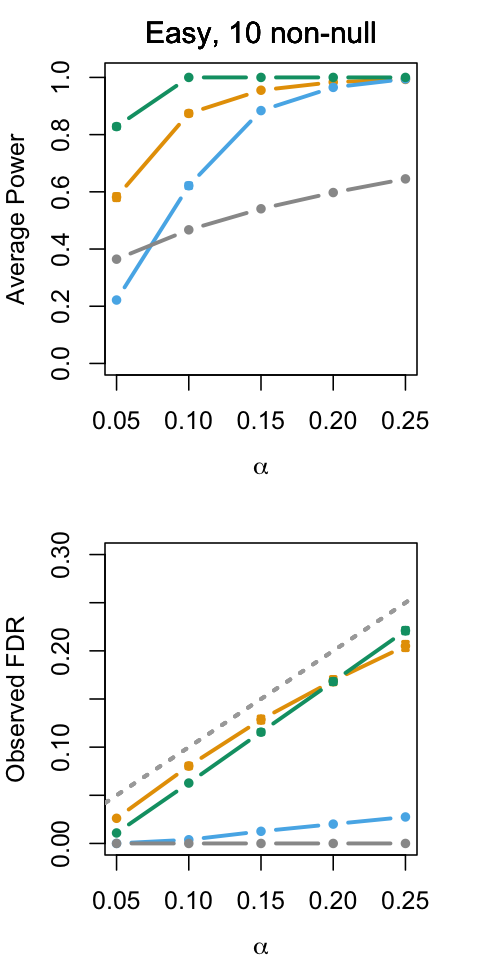
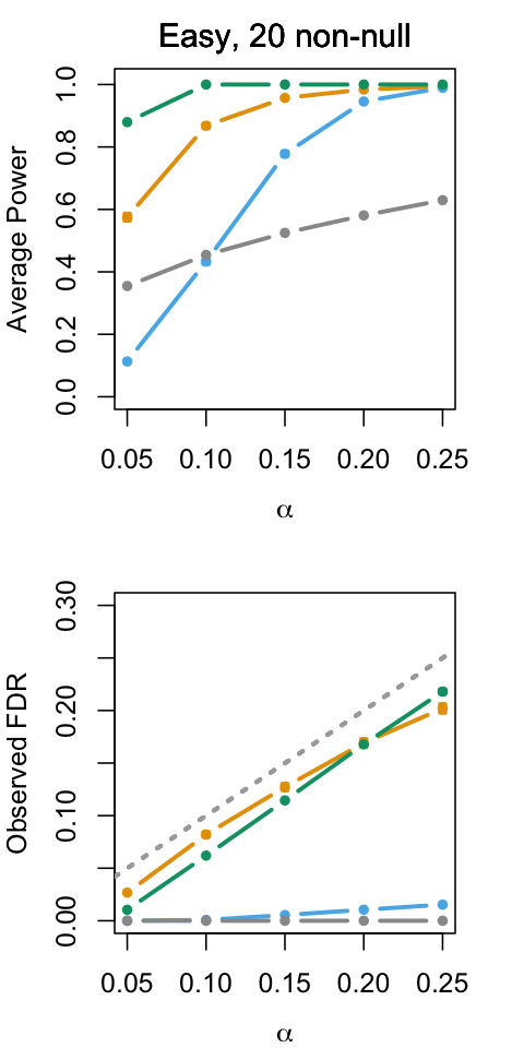
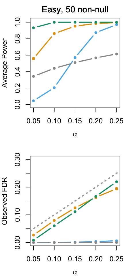
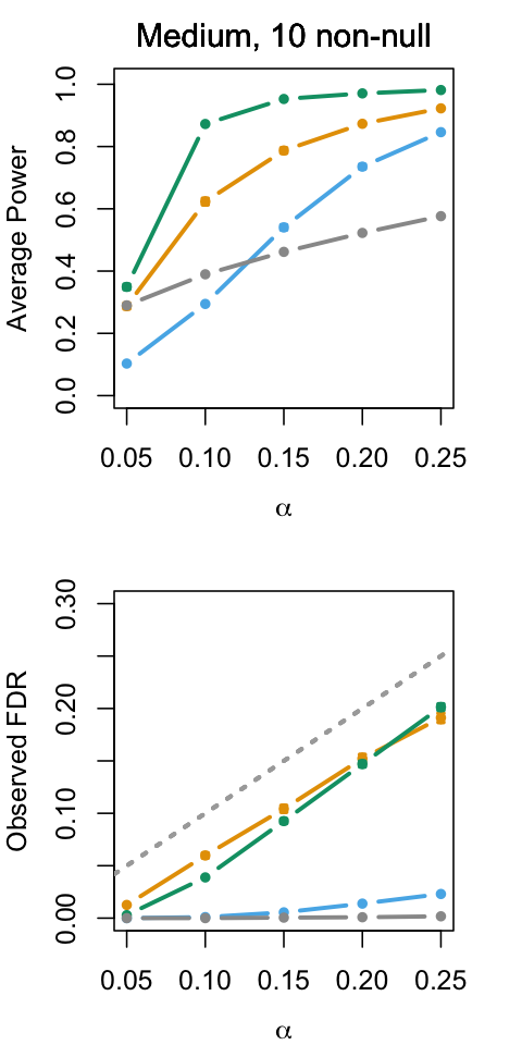
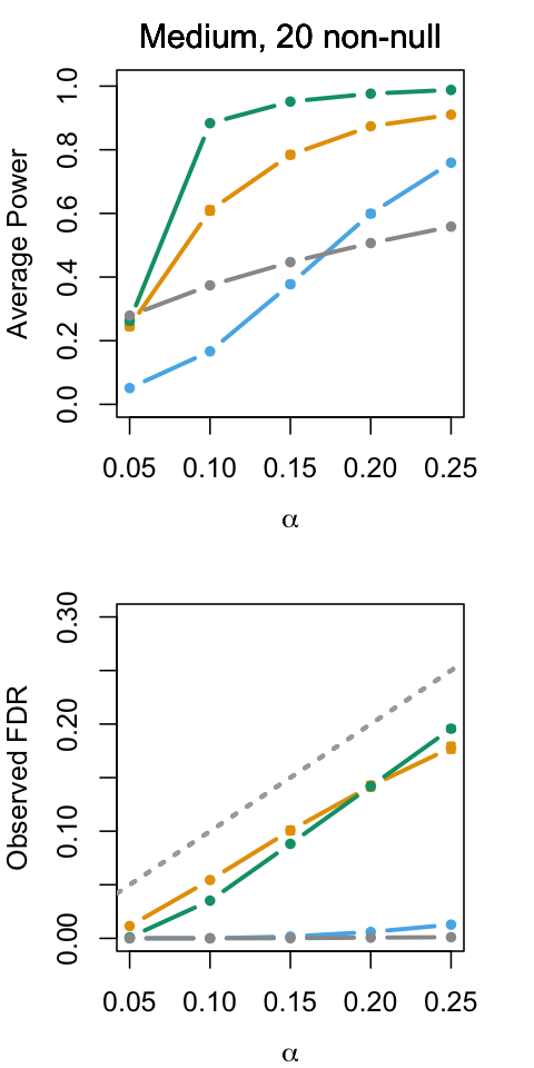
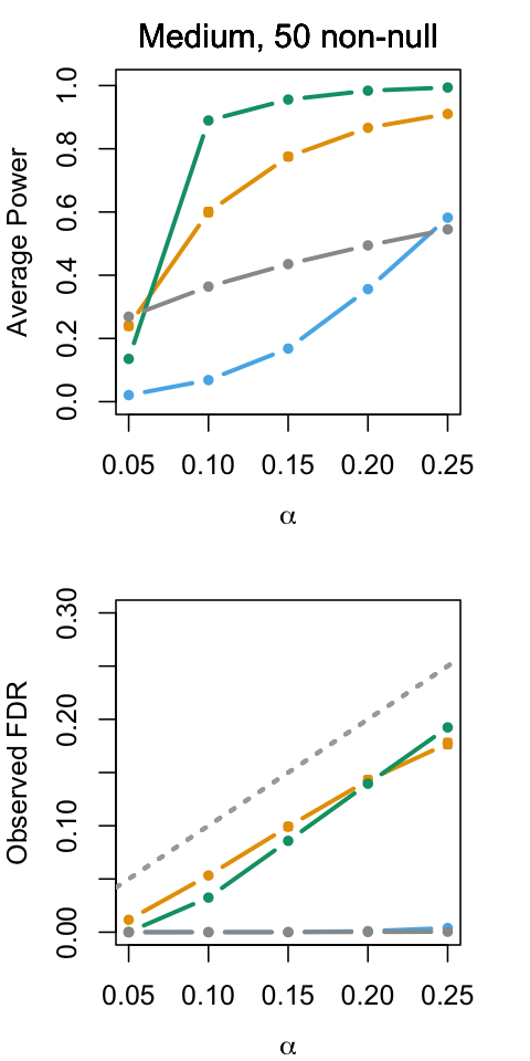
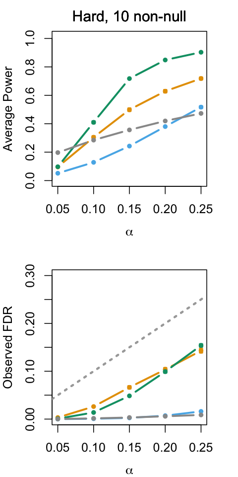
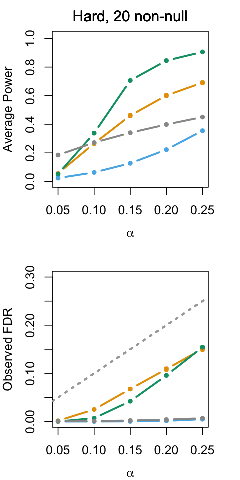
In this section, we demonstrate the performance of our methods in three simulation settings of varying difficulty. The simulation settings consist of ordered hypotheses where the separation of the null and non-null hypotheses is varied to determine the difficulty of the scenario. Additional simulations are provided in Appendix B.

Figure 2: Observed $p$-values for $50$ realizations of the ordered hypothesis simulations described in Section 3. $p$-values corresponding to non-null hypotheses are shown in orange, while those corresponding to null hypotheses are shown in gray. The smooth black curve is the average proportion of null hypotheses up to the given index, and is shown to help gauge the difficulty of the problem. This curve can be thought of as the FDR of a fixed stopping rule which always stops at exactly the given index. Non-null $p$-values are drawn from a $\mathrm{Beta}(1,b)$ distribution, with $b=23,14,8$ for the easy, medium and hard settings, respectively.

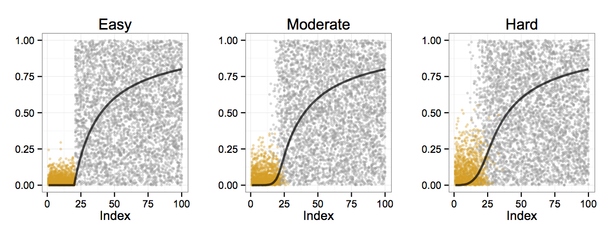
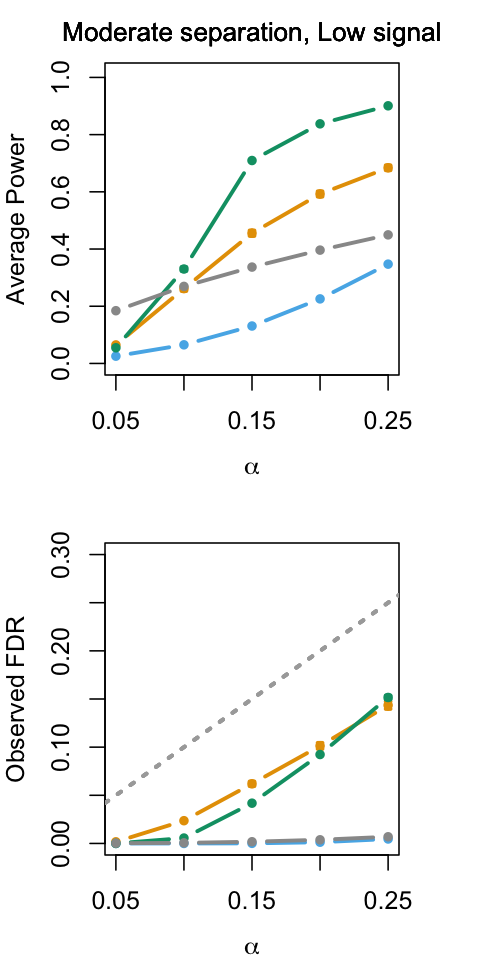
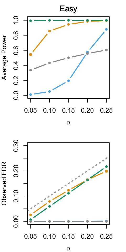
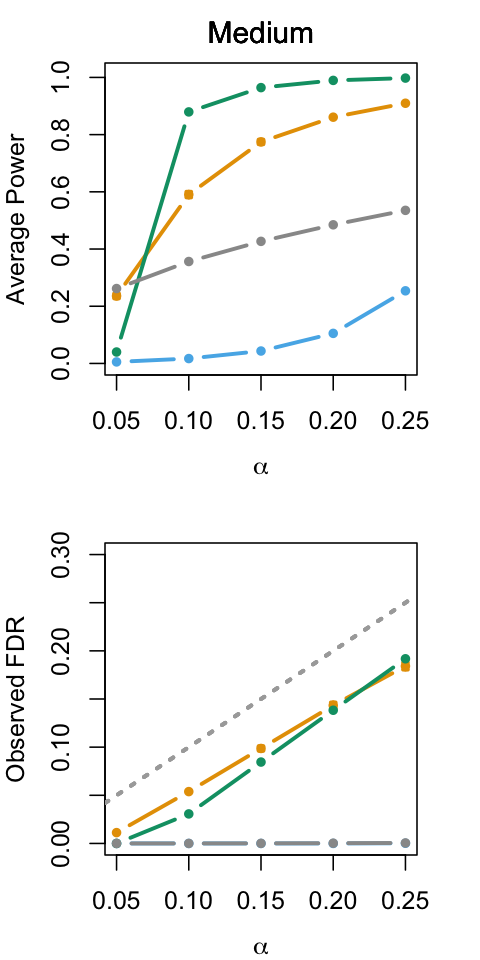
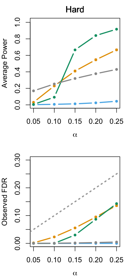
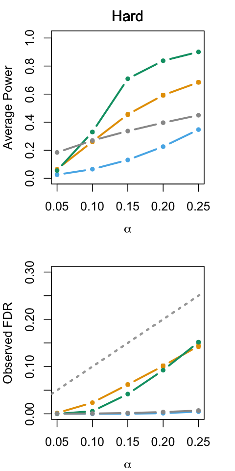
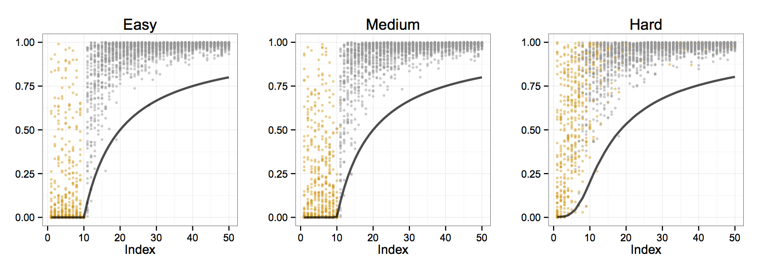
We consider a sequence of $m=100$ hypotheses of which $s=20$ are non-null. The $p$-values corresponding to the non-null hypotheses are drawn from a $\mathrm{Beta}(1,\beta)$ distribution, while those corresponding to true null hypotheses are $U([0,1])$. At each simulation iteration, the indices of the true null hypotheses are selected by sampling without replacement from the set $\{1,2,\ldots,m=100\}$ with probability of selection proportional to $i^{\gamma}$. In this scheme, lower indices have smaller probabilities of being selected. We present results for three simulation cases, which we refer to as ‘easy’ (perfect separation), ‘medium’ ($\gamma=8$), and ‘hard’ ($\gamma=4$). In the easy setup, we have strong signal $b=23$ and all the non-null hypotheses precede the null hypotheses, so we have perfect separation. In the medium difficulty setup, $b=14$ and the null and non-null hypotheses are lightly inter-mixed. In the hard difficulty setup, $b=8$ and the two are much more inter-mixed.

Figure 3: Average power and observed FDR level for the ordered hypothesis example based on 2000 simulation instances. The notion of power used here is that of average power, defined as the fraction of non-null hypotheses that are rejected (i.e., $(k-V)/s$). All four stopping rules successfully control FDR across the three difficulty settings. StrongStop and $\alpha$-thresholding are both very conservative in terms of FDR control. Even though ForwardStop and $\alpha$-investing have similar observed FDR curves, ForwardStop emerges as the more powerful method, and thus has better performance in terms of a precision-recall tradeoff.

For comparison, we also apply the following two rejection rules:

1. Thresholding at $\alpha$. We reject all hypotheses up to the first time that a $p$-value exceeds $\alpha$. This is guaranteed to control FWER and FDR at level $\alpha$ (Marcus et al., 1976).

2. $\alpha$-investing. We use the $\alpha$-investing scheme of Foster and Stine (2008). While this procedure is not generally guaranteed to yield rejections that obey the ordering restriction, we can select parameters for which it does. In particular, defining an investing rule such that the wealth is equal to zero at the first failure to reject, we get

   $$\hat{k}_{invest} =\min\left\{k:p_{k+1}>\frac{(k+1)\alpha}{1+(k+1)\alpha}\right\}.$$

   This is guaranteed to control $\mathbb{E}V/(\mathbb{E}R+1)$ at level $\alpha$. We note that, using generalized $\alpha$-investing (Aharoni and Rosset, 2013), we could tweak the $\alpha$-investing procedure to have more power to reject the earliest hypotheses and less power for further ones; however, we will not explore that possibility here.

These are the best competitors we are aware of for our problem. We emphasize that, unlike ForwardStop and StrongStop, these rules stop at the first $p$-value that exceeds a given threshold. Thus, these methods will fail to identify true rejections with very small $p$-values when they are preceded by a few medium-sized $p$-values.

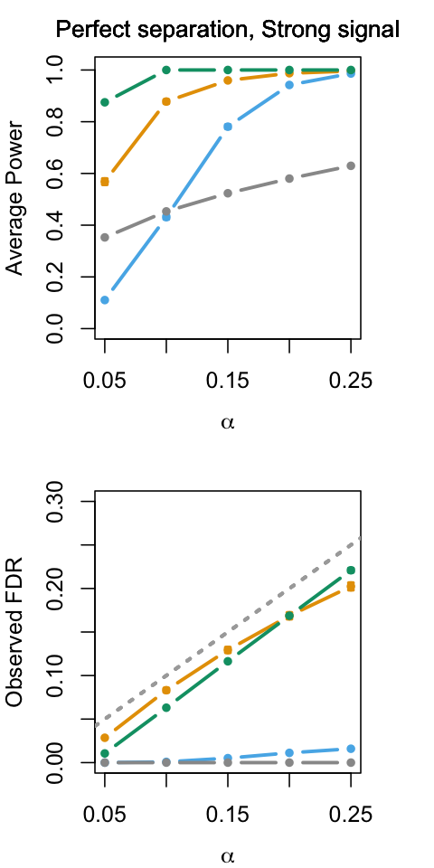
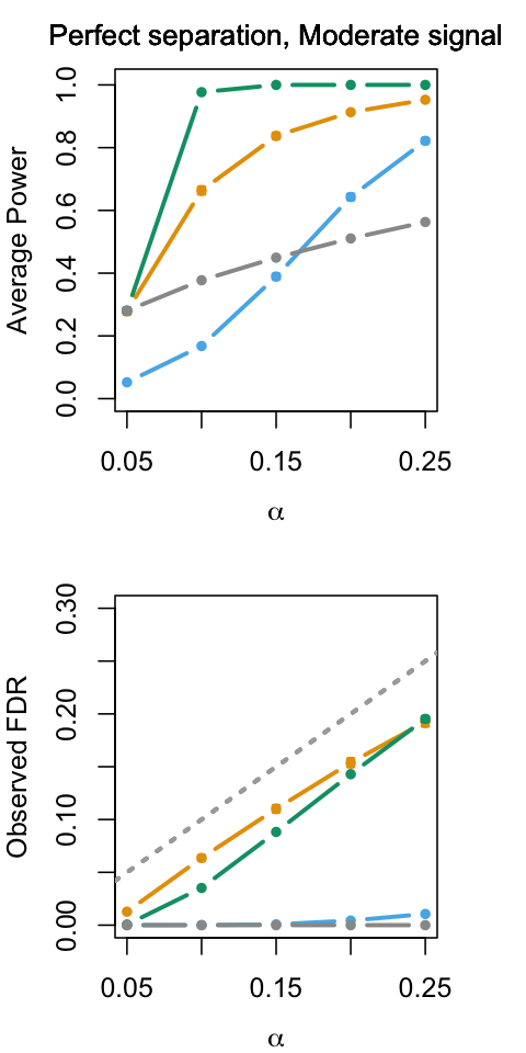
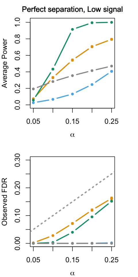
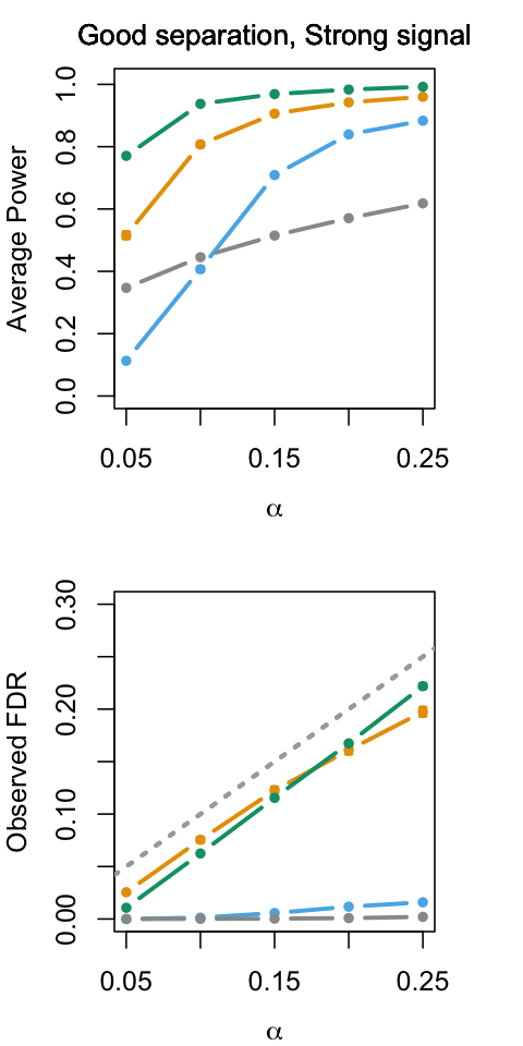
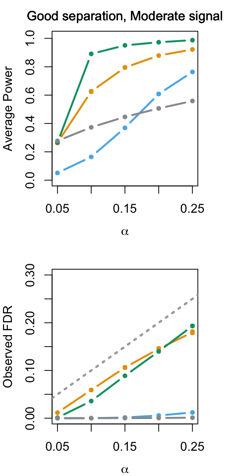
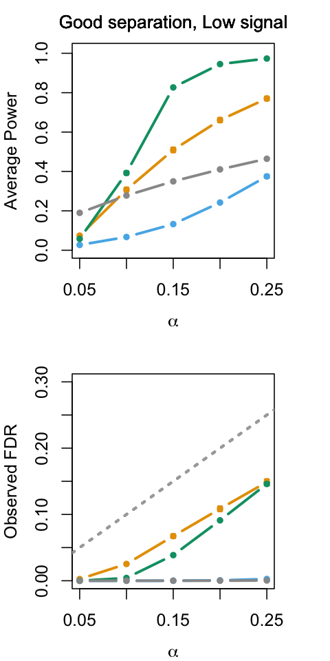
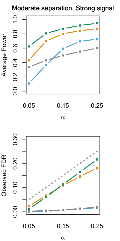
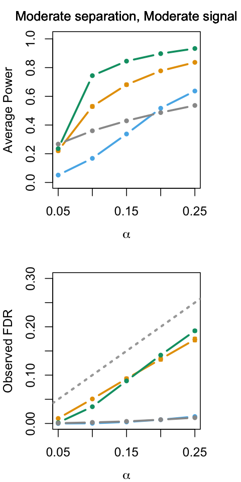
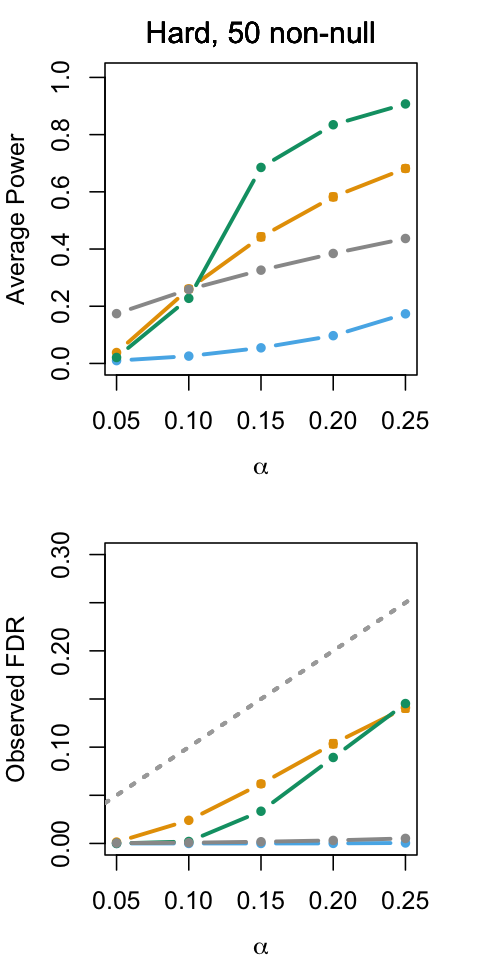
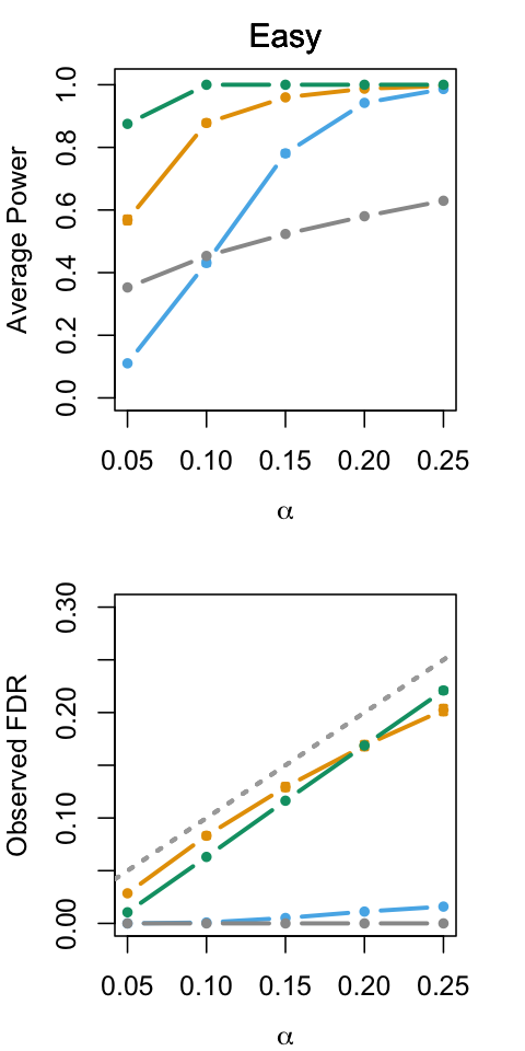
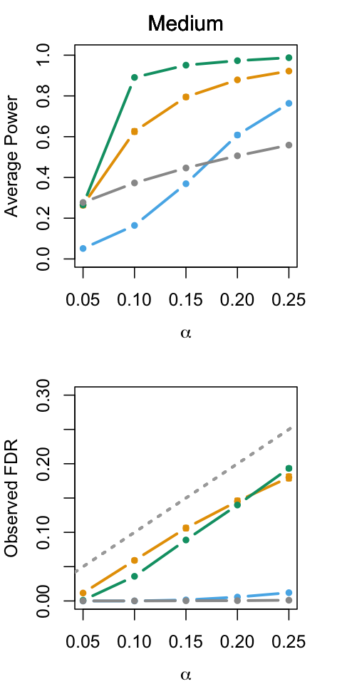
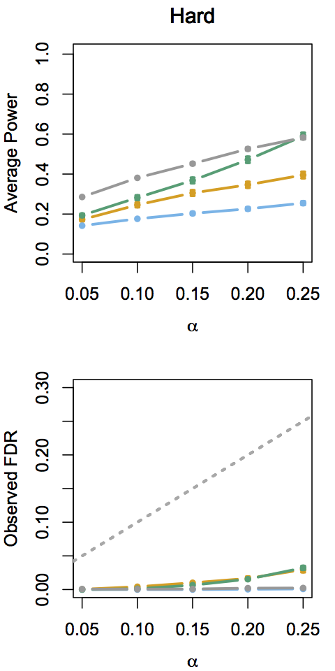
Figure 2 shows scatterplots of observed $p$-values for 50 realizations of the three setups. Figure 3 summarizes the performance of the four stopping rules. We note that StrongStop appears to be more powerful than other methods weak signal/low $\alpha$ settings. This may occur because, unlike the other methods, StrongStop scans $p$-values back-to-front and is therefore less sensitive to the occurrence of large $p$-values early in the alternative.

4 Model Selection and Ordered Testing

We now revisit the application that motivated our ordered hypothesis testing formalism. As discussed in Section 1.1, we assume that a path-based regression procedure like forward stepwise regression or least-angle regression has given us a sequence of models $\emptyset=\mathcal{M}_{0}\subset\mathcal{M}_{1}\subset\ldots\subset\mathcal{M}_{p}$, and our task is is to select one of these nested models. This results in an ordered hypothesis testing problem that is conditional on the order in which the regression algorithm adds variables along its path.

We gave two options for formalizing the hypothesis that $\mathcal{M}_{k}$ improves over $\mathcal{M}_{k-1}$ and that the $k$-th variable should be added to the model: the incremental null (1) and the complete null (3). In this section, we review recent proposals by Taylor et al. (2014) and Lockhart et al. (2014) for testing each of these nulls in the case of least-angle regression and the lasso respectively, and show how to incorporate them into our framework.

We emphasize again that the field of ordered hypothesis testing appears to be growing rapidly, and that the applicability of our sequential FDR controlling procedures is not limited to the tests surveyed here; for example, if we wanted to test $H_{k}^{\text{comp}}$ for forward stepwise regression or the graphical lasso, we could use the test statistics of Loftus and Taylor (2014) or G’Sell et al. (2013) respectively.

4.1 Testing the Incremental Null for Least-Angle Regression

In the context of least-angle regression, Taylor et al. (2014) provide exact, finite sample $p$-values for $H_{k}^{\text{inc}}$ for generic design matrices $X$. The corresponding test statistic is called the spacing test. The first spacing test statistic $T_{1}$ has a simple form

$$T_{1}=\left(1-\Phi\left(\frac{\lambda_{1}}{\sigma}\right)\right)\,\Big{/}\,\left(1-\Phi\left(\frac{\lambda_{2}}{\sigma}\right)\right),$$ (21)

where $\lambda_{1}$ and $\lambda_{2}$ are the first two knots along the least-angle regression path and $\sigma$ is the noise scale. Given a standardized design matrix $X$ and the null hypothesis $H_{1}^{k}$, $T_{1}$ is uniformly distributed over $[0,\,1]$. Remarkably, this result holds under general position conditions on $X$ that hold almost surely if $X$ is drawn from a continuous distribution, and does not require $n$ or $p$ to be large.

Taylor et al. (2014) also derive similar test statistics $T_{k}$ for subsequent steps along the least-angle regression path, which can be used for testing $H_{K}^{\text{inc}}$. Assuming Gaussian noise, all the $H_{k}^{\text{inc}}$-null $p$-values produced by this test are 1-dependent and uniformly distributed over $[0,\,1]$. For the purpose of our demonstrations, we apply our general FDR control procedures directly as though the $p$-values were independent. Developing a version of the spacing test that yields independent $p$-values remains an active area of research.

4.2 Testing the Complete Null for the Lasso

We also apply our formalism to testing the complete null for the lasso path, using the covariance test statistics of Lockhart et al. (2014). As our experiments will make clear, an advantage of testing the complete null instead of the incremental null is the substantial increase in power.

In the case of orthogonal $X$, the covariance test statistics have the particularly simple form

$$T_{k}=\lambda_{k}(\lambda_{k}-\lambda_{k+1}),$$ (22)

where $\lambda_{1}\geq\lambda_{2}\geq\dots$ denote the knots of the lasso path. Because $X$ is orthogonal, the lasso never removes variables along its path, and so we know there will be exactly $p$ knots. Lockhart et al. (2014) show that these test statistics satisfy the following asyptotic guarantee. Recalling that the complete hypotheses are nested, suppose that $H_{1}^{\text{comp}}$, …, $H_{s}^{\text{comp}}$ are false, and $H_{s+1}^{\text{comp}}$ is true. Then, in the limit with $s$ fixed $n,\,p\rightarrow\infty$,

$$\left(T_{s+1},\,...,\,T_{s+\ell}\right)\Rightarrow\left(\operatorname{Exp}(1),\,\operatorname{Exp}\left(\frac{1}{2}\right),\,...,\,\operatorname{Exp}\left(\frac{1}{\ell}\right)\right)$$ (23)

for any fixed $\ell\geq 1$. As shown below, we can use the harmonic asymptotics of these test statistics to improve the power of our sequential procedures.

The major limitation of the statistics (22) is that their distribution can only be controlled asymptotically, and for orthogonal $X$. Lockhart et al. (2014) also provide adaptations of (22) that hold for non-orthogonal $X$; however, the required asymptotic regime is then quite stringent so we may prefer to use finite-sample-exact tests of Taylor et al. (2014) discussed in Section 4.1. In the future, it may be possible to use ideas from Fithian et al. (2014) to devise non-asymptotic and powerful tests of $H_{k}^{\text{comp}}$ for generic $X$.

4.2.1 False Discovery Rate Control for Harmonic Test Statistics

Motivated by the harmonic form of the test statistics $T_{k}$ in (23), we show here how to improve the power of our sequential procedures in this setting. Similar harmonic asymptotics also arise in other contexts, e.g., the test statistics for the graphical lasso of G’Sell et al. (2013).

Abstracting away from concrete regression problems, suppose that we have a sequence of arbitrary statistics $T_{1},\,...,\,T_{m}\geq 0$ corresponding to $m$ hypotheses. The first $s$ test statistics correspond to signal variables; the subsequent ones are independently distributed as

$$\left(T_{s+1},\,...,\,T_{m}\right)\sim\left(\operatorname{Exp}(1),\,\operatorname{Exp}\left(\frac{1}{2}\right),\,...,\,\operatorname{Exp}\left(\frac{1}{m-s}\right)\right),$$ (24)

where $\operatorname{Exp}(\mu)$ denotes the exponential distribution with mean $\mu$. As before, we wish to construct a stopping rule that controls the FDR.

To apply either ForwardStop or StrongStop using $p$-values based on (24) would require knowledge of the number of signal variables $s$, and hence would not be practical. Fortuitously, however, an extension of this idea yields a variation of StrongStop that does not require knowledge of $s$ and controls FDR. Under (24), we have $j\cdot T_{s+j}\sim\operatorname{Exp}(1)$. Using this fact, suppose that we knew $s$ and formed the StrongStop rule for the $m-s$ null test statistics. This would suggest a test based on

$$q^{*}_{i}=\exp\left[-\sum_{j=i}^{m}\frac{\max\{1,\,j-s\}}{j}\,T_{j}\right]$$ (25)

This is not a usable test, since it depends on knowledge of $s$. Now suppose we set $s=0$, giving

$$q^{*}_{i}=\exp\left[-\sum_{j=i}^{m}T_{j}\right]$$ (26)

An application of the BH procedure to the $q_{i}^{*}$ leads to the following rule.

Procedure 3 (TailStop)

Let $q_{i}^{*}$ be defined as in (26). We reject hypotheses $1,\,...,\,\hat{k}_{T}$, where

$$\hat{k}_{T}=\max\left\{k:q^{*}_{k}\leq\frac{\alpha k}{m}\right\}.$$ (27)

Now the choice $s=0$ is anti-conservative (in fact, it is the least conservative possibility for $s$), and so as expected we lose the strong control property of StrongStop. But surprisingly, in the idealized setting of (24), TailStop controls the FDR nearly exactly.

Theorem 4

Given (24), the rule from (27) controls FDR at level $\alpha$. More precisely,

$$\mathbb{E}\left[{\left(\hat{k}_{T}-s\right)_{+}}\,\Big{/}\,{\max\left\{\hat{k}_{T},1\right\}}\right]=\alpha\,\frac{m-s}{m}.$$

The name TailStop emphasizes the fact that this procedure starts scanning the test statistics from the back of the list, rather than from the front. Scanning from the back allows us to adapt to the harmonic decay of the null $p$-values without knowing the number $s$ of non-null predictors. An analogue to ForwardStop for this setup would be much more difficult to implement, as we would need to estimate $s$ explicitly. We emphasize that the guarantees from Theorem 4 hold under the generative model (24), whereas the covariance test statistics only have this distribution asymptotically. However, in our simulation experiments, the asymptotic regime appears to hold well enough for this not to be an issue.

5 Model Selection Experiments

Figure 4: Observed $p$-values for $H_{k}^{\text{inc}}$ in $50$ realizations of the spacing test (Taylor et al., 2014) for least-angle regression. $p$-values corresponding to non-null hypotheses are shown in orange, while those corresponding to null hypotheses are shown in gray. The smooth black curve is the average proportion of null hypotheses up to the given index. This example is similar to the Easy setting of the ordered hypothesis example of §3 in that the null and alternative are nearly perfectly separated. However, in the least-angle regression setting the $p$-values under the alternative are highly variable and can be quite large, particularly in the Hard setting.

In this section, we use the sequential procedures from 2 for pathwise model selection in sparse regression. As discussed in Section 4, we focus on two particular problems: testing the incremental null for least-angle regression with generic design (Section 5.1), and testing the complete null for the lasso with orthogonal design (Section 5.2).

The first of these two settings is of course more immediately relevant to practice, and we verify that ForwardStop paired with the spacing test statistics of Taylor et al. (2014) performs well on a real medical dataset. Meanwhile, the orthogonal simulations in Section 5.2 showcase the power boost that we can obtain from testing the complete null instead of the incremental null. We believe that further theoretical advances in the pathwise testing literature will enable us to have similar power along with FDR guarantees in finite sample with generic $X$.

Finally, although our testing procedures are mathematically motivated by different null hypotheses, namely the incremental and complete ones, we evaluate the performance of each method in terms of its full-model false discovery rate (that is, the fraction of selected variables that do not belong to the support of the true $\beta^{*}$). This lets us make a more direct practical comparison between different methods.

5.1 Testing the Incremental Null for Least-Angle Regression

Figure 5: Average power and observed FDR level for the spacing test $p$-values for $H_{k}^{\text{inc}}$ (Taylor et al., 2014). Even though there is nearly perfect separation between the null and alternative regions, the presence of large alternative $p$-values early in the path makes this a difficult problem. StrongStop attains both the highest average power and the lowest observed FDR across the simulation settings. Unlike the other methods, StrongStop scans $p$-values back-to-front, and is therefore able to perform well despite the occurrence of large $p$-values early in the path.

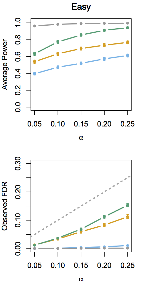
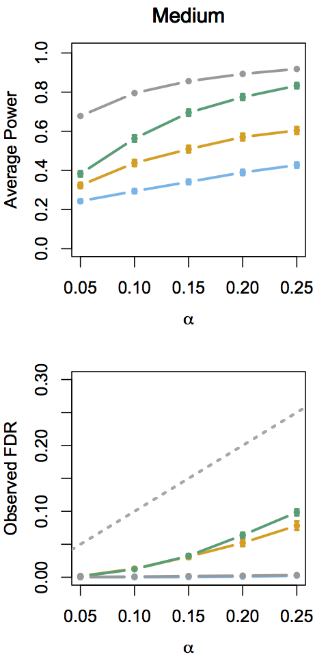
We compare the performance of ForwardStop, StrongStop, $\alpha$-investing and $\alpha$-thresholding on the spacing test statistics from Section 4.1. We try three different simulation settings with varying signal strength. TailStop is not included in this comparison because it should only be used when the null test statistics exhibit harmonic behaviour as in (23), whereas the spacing test $p$-values are uniform.

In all three settings we have $n=200$ observations on $p=100$ variables of which $10$ are non-null, and standard normal errors on the observations. The design matrix $X$ is taken to have iid Gaussian entries. The non-zero entries of the parameter vector $\beta$ are taken to be equally spaced values from $2\gamma$ to $\gamma\sqrt{2\log p}$, where $\gamma$ is varied to set the difficulty of the problem.

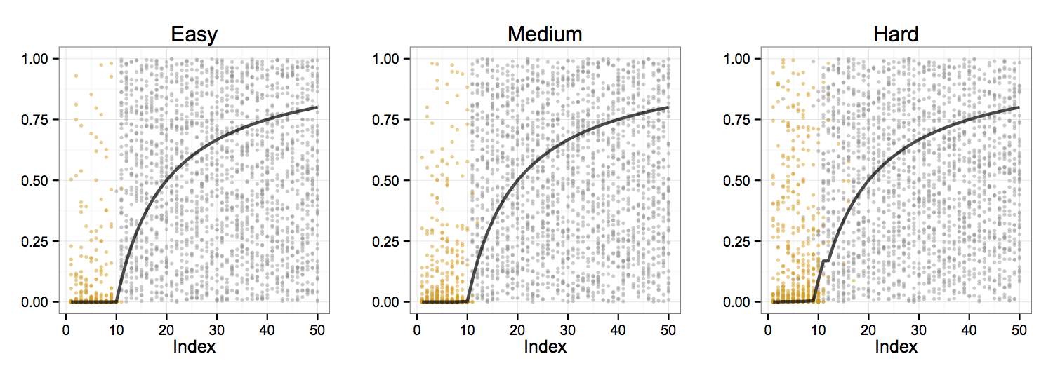
Figure 4 shows $p$-values from 50 realizations of each simulation setting. Note that while all three settings have excellent separation—meaning that least-angle regression selects most of the signal variables before admitting any noise variables—the $p$-values under the alternative can still be quite large. Figure 5 shows plots of average power and observed FDR level across the three simulation settings.

5.1.1 HIV Data

Figure 6: The $H_{k}^{\text{inc}}$ $p$-values from the spacings test for the least-angle regression path, applied to the Abacavir resistance data of Rhee et al. (2006). The vertical lines mark the stopping points of the four stopping rules, all with $\alpha=0.2$. ForwardStop selects the first 16 variables, even though the $p$-values at 9 and 14 are quite high. All but one the selections made by ForwardStop are considered meaningful by a previous study (Rhee et al., 2005).

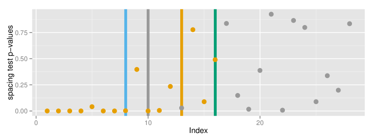
As a practical demonstration of our methods, we apply the same approach to the Human Immunodeficiency Virus Type 1 (HIV-1) data of Rhee et al. (2006), which studied the genetic basis of HIV-1 resistance to several antiretroviral drugs. We focus on one of the accompanying data sets, which measures the resistance of HIV-1 to six different Nucleoside RT inhibitors (a type of antiretroviral drug) over 1005 subjects with mutations measured at 202 different locations (after removing missing and duplicate values). The paper sought to determine which particular mutations were predictive of resistance to these drugs.

In this section, we use least-angle regression to estimate a sparse linear model predicting drug resistance from the mutation marker locations. The ForwardStop, StrongStop, $\alpha$-investing, and $\alpha$-thresholding stopping rules are applied to the $H_{k}^{\text{inc}}$ $p$-values from the spacing test described in Section 4.1 to select a model along the least-angle regression path. A previous study of Rhee et al. (2005) provides a list of known relationships between mutations and drug resistance, which allows partial assessment of the validity of the selected variables. This data set has also been studied by Barber and Candes (2014) in order to assess the performance of the knockoff filter for variable selection; the main difference is that, unlike us, they do not constrain the selection set to be the beginning of the least-angle regression path.

Table 2: Number of selections ($R$) made on the drug resistance data of Rhee et al. (2006) using least-angle regression, the $p$-values from the spacings tests, and the four stopping rules (with $\alpha=0.2$). The number of the correctly selected mutation locations ($S$) is assessed using results from a previous study. ForwardStop and StrongStop have the most competitive power, with the advantage varying by drug. The abbreviations match those used in the original paper.

	3TC		ABC		AZT		D4T		DDI		TDF
Rule	$R$	$S$	$R$	$S$	$R$	$S$	$R$	$S$	$R$	$S$	$R$	$S$
ForwardStop	4	4	16	15	4	4	18	14	3	3	6	6
StrongStop	4	4	10	10	8	8	10	9	12	12	6	6
$\alpha$-Thresholding	4	4	8	8	4	4	10	9	3	3	2	2
$\alpha$-Investing	4	4	13	12	4	4	21	14	3	3	2	2

Table 2 shows the number of rejections and number of correct rejections for each method applied to each of the six drug resistance outcomes. For illustration, we plot the $p$-values and stopping points for resistance to Abacavir (ABC) in Figure 6. The theory supporting ForwardStop and StrongStop suggest that the selected models should contain no more than 20% false positives in expectation. The information available from the literature supports the validity of the selections, showing that the variables selected by our procedures largely corresponded to meaningful relationships based on previous studies conducted with independent data. We observe that, while all methods appear to achieve overall FDR control, in each case either ForwardStop or StrongStop yield the highest number of correct rejections.

5.2 Testing the Complete Null for the Lasso with Orthogonal $X$

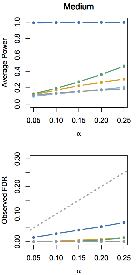
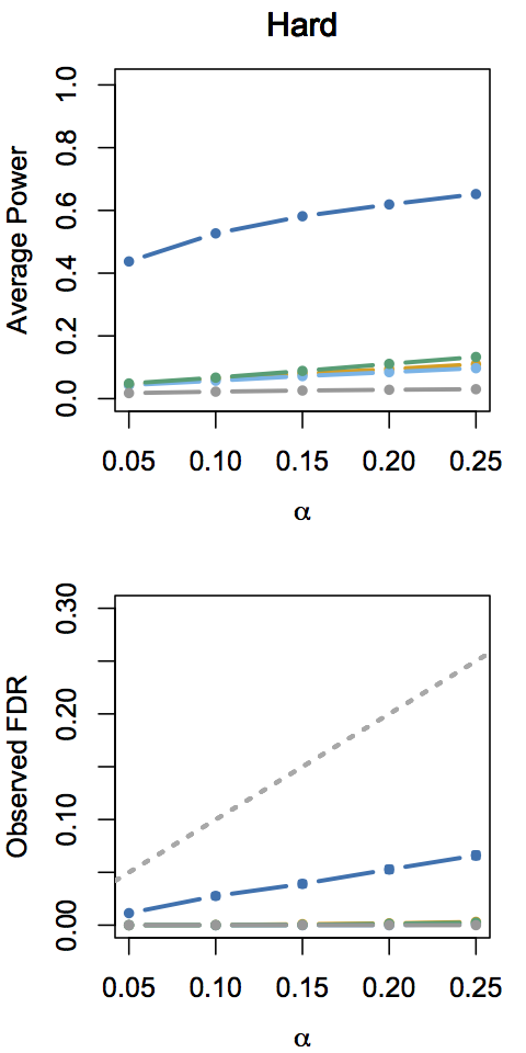
In this section, we compare the performance of StrongStop, ForwardStop, $\alpha$-investing, $\alpha$-thresholding, as well as TailStop for testing the complete null for the lasso with orthogonal $X$ using the covariance test statistics of Lockhart et al. (2014). As discussed in Section 4.2, these test statistics exhibit a harmonic behavior that TailStop is designed to take advantage of. All other procedures operate on conservative $p$-values, $p_{j}=\exp(-T_{j})$, obtained by bounding the null distributions by $\operatorname{Exp}(1)$.

Figure 7: Observed $p$-values for $50$ realizations of the covariance test (Lockhart et al., 2014) for $H_{k}^{\text{comp}}$ with orthogonal $X$. $p$-values corresponding to non-null hypotheses are shown in orange, while those corresponding to null hypotheses are shown in gray. The smooth black curve is the average proportion of null hypotheses up to the given index. Note that these $p$-values behave very differently from those in the ordered hypothesis example presented in §3. The null $p$-values here exhibit $\operatorname{Exp}(1/\ell)$ behaviour, as described in §4.2. Note that the non-null $p$-values for this test can be quite large on occasion. TailStop performs well in part because it is not sensitive to the presence of some large non-null $p$-values.

We consider three scenarios which we once again refer to as easy, medium and hard. In all of the settings we have $n=200$ observations on $p=100$ variables of which $10$ are non-null, and standard normal errors on the observations. The non-zero entries of the parameter vector $\beta$ are taken to be equally spaced values from $2\gamma$ to $\gamma\sqrt{2\log p}$, where $\gamma$ is varied to set the difficulty of the problem. Figure 7 shows $p$-values from 50 realizations of each simulation setting; they exhibit harmonic behavior as described in Section 4.2.

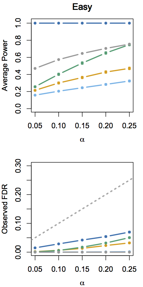
Figure 8 shows plots of average power and observed FDR level across the three simulation settings. The superior performance of TailStop is both desirable and expected, as it is the only rule that can take advantage of the rapid decay of the test statistics in the null.

Figure 8: Average power and observed FDR level for the orthogonal lasso using the covariance test of Lockhart et al. (2014) for $H_{k}^{\text{comp}}$. In the bottom panels, we see that all methods control the FDR. However, in the medium and hard settings TailStop is the only method that shows sensitivity to the choice of target $\alpha$ level. All other methods have an observed FDR level that’s effectively $0$, irrespective of the target $\alpha$. From the power plots we also see that TailStop has far higher power than the other procedures — in the medium setting at low $\alpha$ the power is almost 10 times higher than any other method. By taking advantage of the $\operatorname{Exp}(1/\ell)$ behaviour of the null p-values, TailStop far outperforms the other methods in power across all the difficulty settings.

6 Conclusions

We have introduced a new setting for multiple hypothesis testing that is motivated by sequential model selection problems. In this setting, the hypotheses are ordered, and all rejections are required to lie in an initial contiguous block. Because of this constraint, existing multiple testing approaches do not control criteria like the False Discovery Rate (FDR).

We proposed a pair of procedures for testing in this setting, denoted by ForwardStop and StrongStop. We proved that these procedures control FDR at a specified level while respecting the required ordering of the rejections. Two procedures were proposed because they provide different advantages. ForwardStop is simple and robust to assumptions on the particular behavior of the null distribution. Meanwhile, when the null distribution is dependable, StrongStop controls not only FDR, but the Family-Wise Error Rate (FWER). We then applied our methods to model selection, and provided a modification of StrongStop, called TailStop, which takes advantage of the harmonic distributional guarantees that are available in some of those settings.

A variety of researchers are continuing to work on developing stepwise distributional guarantees for a wide range of model selection problems. As many of these procedures are sequential in nature, we hope that the stopping procedures from this paper will provide a way to convert these stepwise guarantees into model selection rules with accompanying inferential guarantees.

There are many important challenges for future work. For exact control of FDR or FWER, our methods require that the null $p$-values be independent. Except under orthogonal design, this is not true for any of the existing sequential $p$-value procedures that we are aware of. Further work is need in extending our theory, and/or developing new sequential regression tests that yield independence under the null.

Appendix A Proofs

Proof A.1 (Lemma 1).

We can map any rejection threshold $t$ to a number of rejections $k$. For the purpose of this proof, we will frame the problem as how to choose a rejection threshold $\hat{t}$; any choice of $\hat{t}\in[0,1]$ immediately leads to a rule

$$\hat{k}_{F}=R(\hat{t})=\left|\{i:q_{i}\leq\hat{t}\}\right|.$$

Similarly, the number of false discoveries is given by $V(\hat{t})=\left|\{i>s:q_{i}\leq\hat{t}\}\right|$. We define the threshold selection rule

$$\hat{t}_{\alpha}=\max\left\{t\in[0,1]:t\leq\frac{\alpha\,R(t)}{m}\right\}.$$

Here, $R(\hat{t}_{\alpha})=\hat{k}_{F}$ and so this rule is equivalent to the one defined in the hypothesis.

When coming in from $0$, $R(t)$ is piecewise continuous with upwards jumps, so

$$\hat{t}_{\alpha}=\frac{\alpha\,R(\hat{t}_{\alpha})}{m},$$

allowing us to simplify our expression of interest:

$$\frac{V(\hat{t}_{\alpha})}{R(\hat{t}_{\alpha})}=\frac{\alpha}{m}\,\frac{V(\hat{t}_{\alpha})}{\hat{t}_{\alpha}}.$$

Thus, in order to prove our result, it suffices to show that

$$\mathbb{E}\left[\frac{V(\hat{t}_{\alpha})}{\hat{t}_{\alpha}}\right]\leq m.$$

The remainder of this proof establishes the above inequality using Rényi representation and a martingale argument due to Storey et al. (2004).

Recall that, by assumption, $p_{s+1},\,...,\,p_{m}\,{\buildrel\text{iid}\over{\sim}\,}U([0,1])$. Thus, we can use Rényi representation to show that

$$\left(Z_{s+1}-Z_{s},\,...,\,Z_{m}-Z_{s}\right) =\left(\frac{Y_{s+1}}{m-s},\,...,\,\sum_{i=s+1}^{m}\frac{Y_{i}}{m-i+1}\right)$$

$$\,{\buildrel d\over{=}}\,\left(E_{1,\,m-s},\,...,\,E_{m-s,\,m-s}\right),$$

where the $E_{i,\,m-s}$ are standard exponential order statistics, and so

$$\left(e^{-(Z_{s+1}-Z_{s})},\,...,\,e^{-(Z_{m}-Z_{s})}\right)$$

are distributed as $m-s$ order statistics drawn from the uniform $U([0,1])$ distribution. Recalling that

$$1-q_{s+i}=(1-q_{s})\,e^{-(Z_{s+i}-Z_{s})},$$

we see that $q_{s+1}$, …, $q_{m}$ are distributed as uniform order statistics on $[q_{s},\,1]$.

Because the last $q_{i}$ are uniformly distributed,

$${M}(t)=\frac{V(t)}{t}$$

is a martingale on $(q_{s},\,1]$ with time running backwards. Here, the relevant filtration $\mathcal{F}_{t}$ tells us which of the $q_{i}$ are strictly greater than $t$; we can also verify that $\hat{t}_{\alpha}$ is a stopping time with respect to this backwards-time filtration. Now, let ${M}^{+}(t)$, $\hat{t}^{+}_{\alpha}$, and $\mathcal{F}_{t}^{+}$ be the right-continuous modifications of the previous quantities (again, with respect to backwards-running time). By the optional sampling theorem

$$\mathbb{E}\left[\min\{M^{+}(\hat{t}^{+}_{\alpha}),\,C\};\hat{t}^{+}_{\alpha}>q_{s}\right]\leq M(1)=\frac{m-s}{1-q_{s}}$$

for any $C\geq 0$; thus, by the (Lebesgue) monotone convergence theorem,

$$\mathbb{E}\left[M^{+}(\hat{t}^{+}_{\alpha});\hat{t}^{+}_{\alpha}>q_{s}\right]\leq\frac{m-s}{1-q_{s}}$$

Moreover, we can verify that

$$\mathbb{E}\left[M^{+}(\hat{t}^{+}_{\alpha});\hat{t}^{+}_{\alpha}>q_{s}\right]=\mathbb{E}\left[M(\hat{t}_{\alpha});\hat{t}_{\alpha}>q_{s}\right],$$

almost surely, and so

$$\mathbb{E}\left[M(\hat{t}_{\alpha});\hat{t}_{\alpha}>q_{s}\right]\leq\frac{m-s}{1-q_{s}}.$$

For all $t>q_{s}$,

$$\frac{V(t)}{t}=\frac{t-q_{s}}{t}M(t)\leq(1-q_{s})\,M(t),$$

and so

$$\mathbb{E}\left[\frac{V(\hat{t}_{\alpha})}{\hat{t}_{\alpha}};\hat{t}_{\alpha}>q_{s}\right]\leq m-s.$$

Meanwhile,

$$\mathbb{E}\left[\frac{V(\hat{t}_{\alpha})}{\hat{t}_{\alpha}}\big{|}\hat{t}_{\alpha}\leq q_{s}\right]=0,\text{ and so, as claimed, }\mathbb{E}\left[\frac{V(\hat{t}_{\alpha})}{\hat{t}_{\alpha}}\right]\leq m.$$

∎

We begin our analysis of ForwardStop (Procedure 1) by showing that it satisfies the same guarantees as the stopping rule (13). Although the following corollary is subsumed by Theorem 2, its simple proof can still be helpful for understanding the motivation behind ForwardStop.

Corollary 5

Under the conditions of Lemma 1, the ForwardStop procedure defined in (15) has FDR is controlled at level $\alpha$.

Proof A.2.

We can extend our original list of $p$-values $p_{1}$, …, $p_{m}$ by appending additional terms

$$\tilde{p}_{m+1},\,\tilde{p}_{m+2},\,...,\,\tilde{p}_{m^{*}}\,{\buildrel\text{iid}\over{\sim}\,}U([0,1])$$

to it. This extended list of $p$-values still satisfies the conditions of Lemma 1, and so we can apply procedure (13) to this extended list without losing the FDR control guarantee:

$$\hat{k}_{F}^{q,m^{*}}=\max\left\{k:\frac{m^{*}q_{k}^{m^{*}}}{k}\leq\alpha\right\}.$$

As we take $m^{*}\rightarrow\infty$, we have

$$\lim_{m^{*}\rightarrow\infty}m^{*}q_{k}^{m^{*}}=\lim_{m^{*}\rightarrow\infty}m^{*}\left(1-\exp\left[-\sum_{j=1}^{k}\frac{Y_{j}}{m^{*}-j+1}\right]\right)=\sum_{j=1}^{k}Y_{j},$$

and so, because the set $[0,\,\alpha]$ is closed, we recover the procedure described in the hypothesis:

$$\lim_{m^{*}\rightarrow\infty}\hat{k}_{F}^{q,m^{*}}=\hat{k}_{F}.$$

Thus, by dominated convergence, the rule $\hat{k}_{F}$ controls the FDR at level $\alpha$. ∎

Proof A.3 (Theorem 2).

The proof of Lemma 1 used quantities

$$Z_{i}=\sum_{j=1}^{i}\frac{Y_{j}}{m-j+1}=\sum_{j=1}^{i}\frac{Y_{j}}{|\{l\in\{j,\,...,\,m\}\}|}$$

to construct the sorted test statistics $q_{i}$. The key difference between the setup of Lemma 1 and our current setup is that we can no longer assume that if the $i^{th}$ hypothesis is null, then all subsequent hypotheses will also be null.

In order to adapt our proof to this new possibility, we need to replace the $Z_{i}$ with

$$Z_{i}^{ALT}=\sum_{j=1}^{i}\frac{Y_{j}}{\nu(j)},\quad\text{where }\nu(j)=|\{l\in\{j,\,...,\,m\}:l\in N\}|,$$

and $N$ is the set of indices corresponding to null hypotheses. Defining

$$q_{i}^{ALT}=1-e^{-Z_{i}^{ALT}},$$

we can use Rényi representation to check that these test statistics have distribution

$$1-q_{i}^{ALT}\,{\buildrel d\over{=}}\,r(i)\,\left(1-U_{\nu(i),\,|N|}\right),\text{ where}$$

$$r(i):=\exp\left[-\sum_{\{j\leq i:j\notin N\}}\frac{Y_{j}}{i}\right]$$

and the $U_{\nu(j),\,|N|}$ are order statistics of the uniform $U([0,1])$ distribution. Here $r(i)$ is deterministic in the sense that it only depends on the location and position of the non-null $p$-values.

If we base our rejection threshold $\hat{t}^{ALT}_{\alpha}$ on the $q_{i}^{ALT}$, then by an argument analogous to that in the proof of Lemma 1, we see that

$$\frac{V\left(\hat{t}^{ALT}_{\alpha}\right)}{\hat{t}^{ALT}_{\alpha}}$$

is a sub-martingale with time running backwards. The key step in showing this is to notice is that, now, the decay rate of $V(t)$ is accelerated by a factor $r^{-1}(i)\geq 1$. Thus, the rejection threshold $\hat{t}^{ALT}_{\alpha}$ controls FDR at level $\alpha$ in our new setup where null and non-null hypotheses are allowed to mix.

Now, of course, we cannot compute the rule $\hat{t}^{ALT}_{\alpha}$ because the $Z_{i}^{ALT}$ depend on the unknown number $\nu(j)$ of null hypotheses remaining. However, we can apply the same trick as in the proof of Corollary 5, and append to our list an arbitrarily large number of $p$-values that are known to be null. In the limit where we append infinitely many null $p$-values to our list, we recover the ForwardStop rejection threshold. Thus, by dominated convergence, ForwardStop controls the FDR even when null and non-null hypotheses are interspersed. ∎

Proof A.4 (Theorem 3).

We begin by considering the global null case. In this case, the $\widetilde{Y}_{i}$ are all standard exponential, and so by Rényi representation the $\tilde{q}_{i}$ are distributed as the order statistics of a uniform $U([0,1])$ random variable. Thus, under the global null, the rule $\hat{k}_{S}$ is just Simes’ procedure (Simes, 1986) on the $\tilde{q}_{i}$. Simes’ procedure is known to provide exact $\alpha$-level control under the global null, so (20) holds as an equality under the global null.

Now, consider the case where the global null does not hold. Suppose that we have $\hat{k}_{S}=k>s$. From the definition of $\tilde{q}_{k}$, we see that $\tilde{q}_{k}$ depends only on $p_{k},\,...,\,p_{m}$, and so the event $\tilde{q}_{k}\leq\alpha k/m$ is just as likely under the global null as under any alternative with less than $k$ non-null $p$-values. Thus, conditional on $s$,

$$\sum_{k=s+1}^{m}\mathbb{P}\left[\hat{k}_{S}=k\big{|}\text{alternative}\right]=\sum_{k=s+1}^{m}\mathbb{P}\left[\hat{k}_{S}=k\big{|}\text{null}\right]\leq\alpha,$$

and so the discussed procedure in fact provides strong control. ∎

Proof A.5 (Theorem 4).

Let $Z^{*}_{i}=\sum_{j=i}^{m}T_{i}$. By Rényi representation,

$$\left(Z^{*}_{s+1},\,...,\,Z^{*}_{m}\right)\sim\left(E_{m-s,\,m-s},\,...,\,E_{1,\,m-s}\right),$$

where the $E_{i,\,j}$ are exponential order statistics. Thus, the null test statistics

$$\left(q^{*}_{s+1},\,...,\,q^{*}_{m}\right)$$

are distributed as $m-s$ order statistics drawn from the uniform $U([0,1])$ distribution. The result of Benjamini and Hochberg (1995) immediately implies that we can achieve FDR control by applying the BH procedure to the $q_{i}^{*}$, and so TailStop controls the FDR. The exact equality follows from the result of Benjamini and Yekutieli (2001). ∎

Appendix B Additional Simulations

In this section we revisit the ordered hypothesis example introduced in Section 3 and present the results of a more extensive simulation study. We explore the following perturbations of the problem:

1. Varying signal strength while holding the level of separation fixed. (Figures 9, 10, 11)

2. Increasing the number of hypotheses while retaining the same proportion of non-null hypotheses (Figure 12)

3. Varying the proportion of non-null hypotheses (Figures 13, 14, 15)

We remind the reader of the three simulation settings introduced in 3, which we termed Easy, Medium and Hard. These settings were defined as follows

Easy

Perfect separation (all alternative precede all null), and strong signal ($\mathrm{Beta}(1,23)$)

Medium

Good separation (mild intermixing of hypotheses), and moderate signal ($\mathrm{Beta}(1,14)$)

Hard

Moderate separation (moderate intermixing hypotheses), and low signal ($\mathrm{Beta}(1,8)$)

All results are based on $2000$ simulation iterations. Unless otherwise specified, the simulations are carried out with $m=100$ total hypotheses of which $s=20$ are non-null.

Figure 9: Effect of signal strength on stopping rule performance: Perfect separation regime. ForwardStop remains the best performing method overall, except at the lowest $\alpha$ level in the moderate and low signal regimes. All of the methods become more conservative as the signal strength decreases.

Figure 10: Effect of signal strength on stopping rule performance: Good separation regime. The effect of signal strength is qualitatively the same as in the perfect separation regime.

Figure 11: Effect of signal strength on stopping rule performance: Moderate separation regime. The effect of signal strength is qualitatively the same as in the perfect separation and good separation regimes.

Figure 12: Effect of increasing the total number of hypotheses. Instead of $100$ hypotheses of which $20$ are non-null, we consider $1000$ hypotheses of which $200$ are non-null. With the exception of $\alpha$-thresholding, the performance of the methods remains largely unchanged. One small change is that ForwardStop loses power around $\alpha=0.1$ in the Hard setting. The key difference is that the performance of $\alpha$-thresholding considerably degrades. This is not surprising when we consider that $\alpha$-thresholding is simply a geometric random variable. Thus as we increase the number of non-null hypotheses we expect the average power of $\alpha$-thresholding to drop to $0$.

Figure 13: Effect of varying the number of non-nulls out of $m=100$ total hypotheses: Easy regime. With the exception of $\alpha$-thresholding, the performance of the methods remains largely unchanged. The performance of $\alpha$-thresholding degrades considerably as the number of non-null hypotheses increases. An explanation for this behaviour is presented in 12.

Figure 14: Effect of varying the number of non-nulls out of $m=100$ total hypotheses: Medium regime. The effect of varying the number of non-null hypotheses is qualitatively the same as in the Easy regime.

Figure 15: Effect of varying the number of non-nulls out of $m=100$ total hypotheses: Hard regime. The effect of signal strength is qualitatively the same as in the Easy and Medium regimes.

References

- Aharoni and Rosset (2013) Aharoni, E. and S. Rosset (2013). Generalized -investing: definitions, optimality results and application to public databases. Journal of the Royal Statistical Society: Series B (Statistical Methodology).
- Akaike (1974) Akaike, H. (1974). A new look at the statistical model identification. Automatic Control, IEEE Transactions on 19(6), 716–723.
- Barber and Candes (2014) Barber, R. F. and E. Candes (2014). Controlling the false discovery rate via knockoffs. arXiv preprint arXiv:1404.5609.
- Benjamini and Gavrilov (2009) Benjamini, Y. and Y. Gavrilov (2009). A simple forward selection procedure based on false discovery rate control. The Annals of Applied Statistics 3(1), 179–198.
- Benjamini and Hochberg (1995) Benjamini, Y. and Y. Hochberg (1995). Controlling the false discovery rate: a practical and powerful approach to multiple testing. Journal of the Royal Statistical Society. Series B (Methodological), 289–300.
- Benjamini and Yekutieli (2001) Benjamini, Y. and D. Yekutieli (2001). The control of the false discovery rate in multiple testing under dependency. Annals of statistics, 1165–1188.
- Blanchard and Roquain (2008) Blanchard, G. and E. Roquain (2008). Two simple sufficient conditions for FDR control. Electronic journal of Statistics 2, 963–992.
- Bogdan et al. (2014) Bogdan, M., E. v. d. Berg, C. Sabatti, W. Su, and E. J. Candes (2014). SLOPE—adaptive variable selection via convex optimization. arXiv preprint arXiv:1407.3824.
- Churchill and Doerge (1994) Churchill, G. A. and R. W. Doerge (1994). Empirical threshold values for quantitative trait mapping. Genetics 138(3), 963–971.
- Consortium et al. (2012) Consortium, . G. P. et al. (2012). An integrated map of genetic variation from 1,092 human genomes. Nature 491(7422), 56–65.
- Efron et al. (2004) Efron, B., T. Hastie, I. Johnstone, and R. Tibshirani (2004). Least angle regression. Annals of Statistics 32(2), 407–499. With discussion, and a rejoinder by the authors.
- Efron et al. (2001) Efron, B., R. Tibshirani, J. Storey, and V. Tusher (2001). Empirical Bayes analysis of a microarray experiment. Journal of the American Statistical Association, 1151–1160.
- Fithian et al. (2014) Fithian, W., D. Sun, and J. Taylor (2014). Optimal inference after model selection. arXiv preprint arXiv:1410.2597.
- Foster and Stine (2008) Foster, D. P. and R. A. Stine (2008). -investing: a procedure for sequential control of expected false discoveries. Journal of the Royal Statistical Society: Series B (Statistical Methodology) 70(2), 429–444.
- Goeman and Solari (2010) Goeman, J. J. and A. Solari (2010). The sequential rejection principle of familywise error control. The Annals of Statistics, 3782–3810.
- G’Sell et al. (2015) G’Sell, M., S. Wager, A. Chouldechova, and R. Tibshirani (2015). Supplementary material: Sequential selection procedures and false discovery rate control. Journal of the Royal Statistical Society: Series B (Statistical Methodology).
- G’Sell et al. (2013) G’Sell, M. G., T. Hastie, and R. Tibshirani (2013). False variable selection rates in regression. arXiv preprint arXiv:1302.2303.
- G’Sell et al. (2013) G’Sell, M. G., J. Taylor, and R. Tibshirani (2013). Adaptive testing for the graphical lasso. arXiv preprint arXiv:1307.4765.
- Hocking (1976) Hocking, R. R. (1976). A biometrics invited paper. The analysis and selection of variables in linear regression. Biometrics, 1–49.
- Lee et al. (2013) Lee, J., D. Sun, Y. Sun, and J. Taylor (2013). Exact post-selection inference with the lasso. arXiv preprint arXiv:1311.6238.
- Lee and Taylor (2014) Lee, J. D. and J. E. Taylor (2014). Exact post model selection inference for marginal screening. In Advances in Neural Information Processing Systems, Volume 27.
- Lin et al. (2011) Lin, D., D. Foster, and L. Ungar (2011). VIF regression: A fast regression algorithm for large data. Journal of the American Statistical Association 106(493), 232–247.
- Lockhart et al. (2014) Lockhart, R., J. Taylor, R. J. Tibshirani, and R. Tibshirani (2014). A significance test for the lasso. Annals of Statistics (with Discussion) 42(2), 413–468.
- Loftus and Taylor (2014) Loftus, J. R. and J. E. Taylor (2014). A significance test for forward stepwise model selection. arXiv preprint arXiv:1405.3920.
- Marcus et al. (1976) Marcus, R., P. Eric, and K. R. Gabriel (1976). On closed testing procedures with special reference to ordered analysis of variance. Biometrika 63(3), 655–660.
- Meinshausen and Bühlmann (2010) Meinshausen, N. and P. Bühlmann (2010). Stability selection. Journal of the Royal Statistical Society: Series B (Statistical Methodology) 72(4), 417–473.
- Rényi (1953) Rényi, A. (1953). On the theory of order statistics. Acta Mathematica Hungarica 4(3), 191–231.
- Rhee et al. (2005) Rhee, S.-Y., W. J. Fessel, A. R. Zolopa, L. Hurley, T. Liu, J. Taylor, D. P. Nguyen, S. Slome, D. Klein, M. Horberg, et al. (2005). HIV-1 protease and reverse-transcriptase mutations: correlations with antiretroviral therapy in subtype B isolates and implications for drug-resistance surveillance. Journal of Infectious Diseases 192(3), 456–465.
- Rhee et al. (2006) Rhee, S.-Y., J. Taylor, G. Wadhera, A. Ben-Hur, D. L. Brutlag, and R. W. Shafer (2006). Genotypic predictors of human immunodeficiency virus type 1 drug resistance. Proceedings of the National Academy of Sciences 103(46), 17355–17360. Data available at http://hivdb.stanford.edu/pages/published_analysis/genophenoPNAS2006/.
- Romano and Shaikh (2006) Romano, J. P. and A. M. Shaikh (2006). Stepup procedures for control of generalizations of the familywise error rate. The Annals of Statistics, 1850–1873.
- Schwarz et al. (1978) Schwarz, G. et al. (1978). Estimating the dimension of a model. The annals of statistics 6(2), 461–464.
- Shah and Samworth (2012) Shah, R. and R. Samworth (2012). Variable selection with error control: Another look at stability selection. Journal of the Royal Statistical Society: Series B (Statistical Methodology).
- Simes (1986) Simes, R. J. (1986). An improved Bonferroni procedure for multiple tests of significance. Biometrika 73(3), 751–754.
- Simonsen and McIntyre (2004) Simonsen, K. L. and L. M. McIntyre (2004). Using alpha wisely: improving power to detect multiple qtl. Statistical applications in genetics and molecular biology 3(1).
- Storey et al. (2004) Storey, J. D., J. E. Taylor, and D. Siegmund (2004). Strong control, conservative point estimation and simultaneous conservative consistency of false discovery rates: a unified approach. Journal of the Royal Statistical Society: Series B (Statistical Methodology) 66(1), 187–205.
- Taylor et al. (2014) Taylor, J., R. Lockhart, R. J. Tibshirani, and R. Tibshirani (2014). Post-selection adaptive inference for least angle regression and the lasso. arXiv preprint arXiv:1401.3889.
- Taylor et al. (2013) Taylor, J., J. Loftus, R. Tibshirani, and R. Tibshirani (2013). Tests in adaptive regression via the Kac-Rice formula. arXiv preprint arXiv:1308.3020.
- Tibshirani (1996) Tibshirani, R. (1996). Regression shrinkage and selection via the lasso. Journal of the Royal Statistical Society Series B 58(1), 267–288.
- Westfall and Young (1993) Westfall, P. H. and S. S. Young (1993). Resampling-based multiple testing: Examples and methods for p-value adjustment. John Wiley & Sons.
- Wu et al. (2007) Wu, Y., D. Boos, and L. Stefanski (2007). Controlling variable selection by the addition of pseudovariables. Journal of the American Statistical Association 102(477), 235–243.