About the use of fidelity to assess quantum resources

Abstract

Fidelity is a figure of merit widely employed in quantum technology in order to quantify similarity between quantum states and, in turn, to assess quantum resources or reconstruction techniques. Fidelities higher than, say, 0.9 or 0.99, are usually considered as a piece of evidence to say that two states are very close in the Hilbert space. On the other hand, on the basis of several examples for qubits and continuous variable systems, we show that such high fidelities may be achieved by pairs of states with considerably different physical properties, including separable and entangled states or classical and nonclassical ones. We conclude that fidelity as a tool to assess quantum resources should be employed with caution, possibly combined with additional constraints restricting the pool of achievable states, or only as a mere summary of a full tomographic reconstruction.

I Introduction

In the last two decades several quantum-enhanced communication protocols and measurement schemes have been suggested and demonstrated. The effective implementation of these schemes crucially relies on the generation and characterization of nonclassical states and operations (including measurements), which represent the two pillars of quantum technology. The assessment of quantum resources amounts to make quantitative statements about the similarity of a quantum state to a target one, or to measure the effectiveness of a reconstruction technique. For these purposes one needs a figure of merit to compare quantum states. Among the possible distance-like quantities that can be defined in the Hilbert space a widely adopted measure of closeness of two quantum states is the Uhlmann Fidelity Uhl defined as

$$F(\rho_{1},\rho_{2})=\left(\hbox{Tr}\sqrt{\sqrt{\rho_{1}}\rho_{2}\sqrt{\rho_{1}}}\right)^{2}$$ (1)

which is linked to the Bures distance $D_{B}(\rho_{1},\rho_{2})=\sqrt{2[1-\sqrt{F}]}$ between the two states $\rho_{1}$ and $\rho_{2}$, and provides bounds to the trace distance fuc99

$$1-\sqrt{F(\rho_{1},\rho_{2})}\leq\frac{1}{2}||\rho_{1}-\rho_{2}||_{1}\leq\sqrt{1-F(\rho_{1},\rho_{2})}\,.$$

Fidelity is bounded to the interval $[0,1]$, and values above a given threshold close to unit, say, 0.9 or 0.99 are usually considered very high. Indeed, this implies that the two states are very close in the Hilbert space, as it follows from the above relations between the fidelity and the Bures and trace distances. On the other hand, neighboring states may not share nearly identical physical properties edvd ; dodonov as one may be tempted to conclude. The main purpose of this paper is to show, on the basis of several examples for qubits and continuous variable (CV) systems, that very high values of fidelity may be achieved by pairs of states with considerably different physical properties, including separable and entangled states or classical and nonclassical ones. Furthermore, we provide a quantitative analysis of this discrepancy.

In order to illustrate the point let us start with a very simple example. Suppose you are given a qubit, aimed at being prepared in the basis state $|0\rangle$, and guaranteed to have either a fidelity to the target state larger than a threshold, say $F>0.9$, or a given fidelity within a confidence interval, say $F=0.925\pm 0.025$. The situation is depicted in Fig. 1 where we show the corresponding regions on the Bloch sphere. As it is apparent from the plots, neighboring states in terms of fidelity are compatible with a relatively large portion of the sphere that includes those states with different physical properties, e.g. the spin component in the $z$ direction.

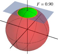
Figure 1: (Color online) The green volumes represent single qubit states having fidelity larger than the threshold $F>0.9$ (left) or a fidelity $F=0.925\pm 0.025$ (right) to the target state $|0\rangle$.

The rest of the paper is devoted to illustrate few relevant, and “more dramatic” examples, for two-qubit states and for continuous variable ones, where fidelity should be employed with caution to assess quantum resources. Indeed, our examples show that high values of fidelity may be achieved by pairs of states with considerably different physical properties, e.g. states containing quantum resources and states of no value for quantum technology. Our examples are thus especially relevant for certification of quantumness in the presence of noise.

The paper is structured as follows. In the next Section we address two-qubit systems, focusing on both entanglement and discord of nearby Pauli diagonal states. The subsequent Sections are devoted to continuous variable systems: Section III addresses certification of quantumness for single-mode squeezed thermal states and their displaced versions, whereas in Section IV we focus on entanglement and discord of two-mode squeezed thermal states. Section V closes the paper with some concluding remarks.

II Two-qubit systems

Let us consider the subset of Pauli diagonal (PD) two-qubit states

$$\rho=\frac{1}{4}\left({\mathbbm{I}}\otimes{\mathbbm{I}}+\sum_{j=1}^{3}c_{j}\sigma_{j}\otimes\sigma_{j}\right)$$ (2)

where $c_{j}$ are real constants, ${\mathbbm{I}}$ is the identity operator and $\sigma_{j}$ are Pauli matrices. The corresponding eigenvalues are

$$\begin{split}\lambda_{0}=\frac{1}{4}\left(1-c_{1}-c_{2}-c_{3}\right)\\ \lambda_{1}=\frac{1}{4}\left(1-c_{1}+c_{2}+c_{3}\right)\\ \lambda_{2}=\frac{1}{4}\left(1+c_{1}-c_{2}+c_{3}\right)\\ \lambda_{3}=\frac{1}{4}\left(1+c_{1}+c_{2}-c_{3}\right)\end{split}$$ (3)

whose positivity implies constraints on coefficients $c_{j}$ for $\rho$ to describe a physical state. PD states in Eq. (2) have maximally mixed marginals (partial traces) $\rho^{A}=\rho^{B}={\mathbbm{I}}/2$, $A$ and $B$ denoting the two subsystems. The choice of this subset stems from the fact that an analytic expression of the quantum discord is available Luo , so we can compare quantum discord and entanglement of states within the PD class for fixed values of fidelity. The fidelity between two PD states may be expressed in terms of the eigenvalues in Eq. (3) as follows

$${F}\left(\rho_{1},\rho_{2}\right)=\Big{(}\sum_{k=0}^{3}\sqrt{\lambda_{k,1}\lambda_{k_{2}}}\Big{)}^{2},$$ (4)

whereas entanglement, quantified by negativity, is given by

$${N}(\rho)=-2\sum_{i}\eta_{i}(\rho^{\tau_{A}}),$$ (5)

where $\eta_{i}(\rho^{\tau_{A}})$ are the negative eigenvalues of the partial transpose $\rho^{\tau_{A}}$ with respect to the subsystem $A$ negativity . The quantum discord for PD states has been evaluated in Luo , and it is given by

$${D}(\rho)={I}(\rho)-\frac{1}{2}(1-c)\log_{2}(1-c)-\frac{1}{2}(1+c)\log_{2}(1+c)$$ (6)

where ${I}(\rho)=2+\sum_{i=0}^{3}\lambda_{i}\log_{2}\lambda_{i}$ is the mutual information and the other terms are the result of the maximization of the classical information. The quantity $c$ denotes the maximum $c\equiv\text{max}\{|c_{1}|,|c_{2}|,|c_{3}|\}$.

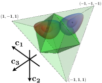
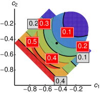
Figure 2: (Color online) (Left panel): The tetrahedron represents the region of all physical PD states, whereas the inner octahedron contains the separable ones. The balloons centered in $c_{1}=c_{2}=c_{3}=-0.45$ (on the right of the panel) contain PD states having fidelity ${F}>0.95$ and $F>0.99$ to the target Werner (entangled) state. The balloons on the left of the panel describe states having fidelity $F>0.95$ and $F>0.99$ to the separable PD state with $c_{1}=0.3$, $c_{2}=-0.3$, and $c_{3}=0.1$ . (Right panel): the plot describes PD states with fixed $c_{3}=-0.45$ and varying $\{c1,c2\}$. We show the ovoidal slice containing states having fidelity ${F}>0.95$ to the target Werner state with $c_{1}=c_{2}=c_{3}=-0.45$ and the corresponding rectangular region of entangled states. Contour lines refer to entanglement negativity (gray) and quantum discord (red).

Let us now consider a situation where the target state of, say, a preparation scheme, is a Werner state

$$\rho_{W}=\frac{1-c}{4}{\mathbbm{I}}\otimes{\mathbbm{I}}+c|\Psi^{-}\rangle\langle\Psi^{-}|\,,$$

i.e. a PD state with $c_{1}=c_{2}=c_{3}=-c$ and $c\in[0,1]$ and where $|\Psi^{-}\rangle=(|01\rangle-|10\rangle)/\sqrt{2}$ is one of the Bell states. The Werner state $\rho_{W}$ is entangled for $c>\frac{1}{3}$ and separable otherwise. In particular, let us choose a target state with $c=0.45$ and address the properties of PD states having fidelity larger than a threshold, say $F>0.95$ or $F>0.99$ to this target. Results are reported in the left panel of Fig. 2, where the tetrahedral region is the region of physical two-qubit PD states and the separable states are confined to the inner octahedron. The ovoidal regions (from now on the balloons) contain the PD states with fidelity ${F}>0.95$ and $F>0.99$ to our target Werner state. As it is apparent from the plot, both the balloons cross the separability border, thus showing that a “high” value of fidelity to the target should not be used as a benchmark for creation of entanglement, even assuming that the generated state belongs to the class of PD states. The same phenomenon may lead one to waste entanglement, i.e. to erroneously recognize an entangled state as separable on the basis of a high fidelity to a separable state, as it may happen to an initially maximally entangled state driven towards the separability threshold by the environmental noise. As an example, we show in the left panel of Fig. 2 the balloons of states with fidelity $F>0.95$ and $F>0.99$ to a separable PD state with $c_{1}=0.3$, $c_{2}=-0.3$, and $c_{3}=0.1$.

In the right panel of Fig. 2 we show the “slice” of PD states with $c_{3}=-0.45$ and fidelity ${F}>0.95$ to the Werner target, together with the corresponding region of entangled states, and the contour lines of entanglement negativity and quantum discord. This plot clearly shows that high values of fidelity are compatible with large range of variation for both entanglement and discord.

The fact that neighboring states may have quite different physical properties has been recently investigated for quantum optical polarization qubits edvd . In particular, the discord of several two-qubit states has been experimentally determined using partial and full polarization tomography. Despite the reconstructed states had high fidelity to depolarized or phase-damped states, their discord has been found to be largely different from the values predicted for these classes of states, such that no reliable estimation procedure beyond tomography may be effectively implemented, and thus questioning the use of fidelity as a figure of merit to assess quantum correlations. Indeed, when full tomography is performed, fidelity is used only to summarize the overall quality of the reconstruction anto1 ; anto2 ; nat1 ; nat2 and thus correctly convey also the information obtained about quantum resources.

III Single-mode Gaussian States

Here we address the use of fidelity to assess quantumness of single-mode CV states. In particular, in Section III.1 we address nonclassicality of squeezed thermal states, whereas Section III.2 is devoted the subPossonian character of their displaced version.

III.1 Squeezed thermal states

Let us now consider single-mode CV systems and start with Gaussian state preparations of the form

$$\rho_{s\mu}=S(r)\nu(N)S^{\dagger}(r)$$ (7)

i.e. single-mode squeezed thermal states (${\hbox{STS}_{1}}$) with real squeezing, $S(r)=\exp\{\frac{1}{2}r(a^{{\dagger}2}-a^{2})\}$ and $N$ thermal photons, $\nu(N)=N^{a^{\dagger}a}/(1+N)^{a^{\dagger}a+1}$. This class of states have zero mean and covariance matrix (CM) given by

$$\sigma=\frac{1}{2\mu}\begin{pmatrix}1/s&0\\ 0&s\end{pmatrix},$$ (8)

where $\mu=(2\sqrt{\det{\sigma}})^{-1}=(2N+1)^{-1}$ is the purity of $\rho_{s\mu}$ and $s=e^{-2r}$ is the squeezing factor. ${\hbox{STS}_{1}}$ are nonclassical, i.e. they show a singular Glauber P-function, when $s<\mu$ or $s>1/\mu$ CTLee . Fidelity between two ${\hbox{STS}_{1}}$ is given by twa96 ; scu98

$$F_{s\mu}=\frac{1}{\sqrt{\Delta+\delta}-\sqrt{\delta}}$$ (9)

where

$$\Delta=\det[\sigma_{1}+\sigma_{2}]\qquad\delta=4\prod_{k=1}^{2}\left[\det[\sigma_{k}]-\frac{1}{4}\right]\,,$$

$\sigma_{1}$ and $\sigma_{2}$ being the CM of the two states. In Fig. 3 we report the region of classicality together with the balloons of ${\hbox{STS}_{1}}$ having fidelity larger than $F_{s\mu}>0.99$ to three ${\hbox{STS}_{1}}$ chosen as targets (one classical thermal state and two nonclassical thermal squeezed states).

As it is apparent from the plot, the balloons have large overlaps with both the classical and the nonclassical region, such that fidelity cannot be used, for this class of states, to certify the creation of quantum resources. This feature is only partially cured by imposing additional constraints to the set of states under examination dodonov . As for example, in the left panel of Fig. 3 we show the “stripes” of states that have both a fidelity $F_{s\mu}>0.99$ and a mean photon numbers $\langle n\rangle$, (i.e. the mean energy of state) which differ at most $10\%$ from that of the target. In the right panel we show the regions of states satisfying also the additional constraints of having photon number fluctuations $\langle\Delta n^{2}\rangle$ within a $10\%$ interval from that of the targets. Overall, we have strong evidence that fidelity should not be used to certify the presence of quantumness, and that this behavior persists even when we add quite stringent constraints to delimit the class of states under investigations. In fact, only by performing the full tomographic reconstruction of the state one imposes a suitable set of constraints to make fidelity a fully meaningful figure of merit Jar09 . In this case, as already mentioned for qubits, fidelity represents a summary of the precision achieved by the full tomographic reconstruction.

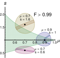
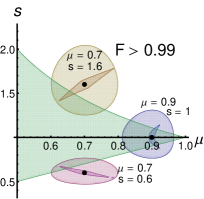
Figure 3: (Color online) The plots show the region of classicality (the triangular-like green regions) together with the balloons of ${\hbox{STS}_{1}}$ having fidelity larger than $F_{s\mu}>0.99$ to three ${\hbox{STS}_{1}}$ chosen as targets: a classical thermal state with $s=1$ and $\mu=0.9$ and two nonclassical ${\hbox{STS}_{1}}$ with $\mu=0.7$ and $s=0.6$ and $s=1.6$ respectively. In the left panel the stripes of states close to the targets contain states having $F_{s\mu}>0.99$ and mean photon numbers which differ at most $10\%$ from that of the target. In the right panel the states close to the targets satisfy the additional constraints of having number fluctuations within a $10\%$ interval from that of the targets.

III.2 Displaced squeezed thermal states

When only intensity measurements may be performed, nonclassicality of a single-mode state may be assessed by the Fano Factor HP82 , which is defined as the ratio of the photon number fluctuations over the mean photon number $R=\langle\Delta n^{2}\rangle/\langle n\rangle$. One has $R=1$ for coherent states, while a smaller value is a signature of nonclassicality since sub-Poissonian statistics cannot be described in classical terms. In order to illustrate the possible drawbacks of fidelity in certifying this form of quantumness, let us consider displaced version of ${\hbox{STS}_{1}}$

$$\rho_{G}=D(x)\rho_{s\mu}D^{\dagger}(x),$$ (10)

where $D(\alpha)=\exp\{\alpha a^{\dagger}-\bar{\alpha}a\}$ is the displacement operator and we chose real displacement $\alpha=x\in{\mathbbm{R}}$. The CM is determined by $\rho_{s\mu}$ whereas the displacement change only the mean values of the canonical operators. The fidelity between two Gaussian states of the form $\rho_{G}$ is given by scu98

$$F_{G}=\exp\{-(\mathbf{X}_{1}-\mathbf{X}_{2})^{T}(\sigma_{1}+\sigma_{2})^{-1}(\mathbf{X}_{1}-\mathbf{X}_{2})\}F_{s\mu}$$ (11)

where $\mathbf{X}=(x,0)$. In the left panel of Fig. 4 we show the region of sub-Poissonianity as a function of the purity, the squeezing factor, and the displacement of states $\rho_{G}$. We also show the balloons of states with fidelity larger than $F_{G}>0.97$ to two $\rho_{G}$ target states: a subPoissonian state corresponding to $\mu=0.9$, $s=1.4$, and $x=0.5$ and a superPoissonian one with $\mu=0.7$, $s=1.2$, and $x=1.5$. Despite the high value of fidelity (notice that fidelity decreases exponentially with the displacement amplitude) both the balloons crosses the Poissonian border, and the parameters of the states that may differ considerably from the targeted ones. In the right panel of Fig. 4 we show the subPoissonian region for a fixed value of purity $\mu=0.8$ as a function of squeezing and displacement, together with the balloons of states having fidelity larger than $F_{G}>0.97$ to a pair of target states: a subPoissonian state with parameters $x=1.5$ and $s=1.5$ and a superPoissonian one with $x=0.8$ and $s=1.0$. We also show the subregions of states having mean photon number and number fluctuations which differ at most $10\%$ from those of the target. We notice that even restricting attention to states with comparable energy and fluctuations, fidelity is not able to discriminate states having quantum resources or not.

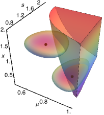
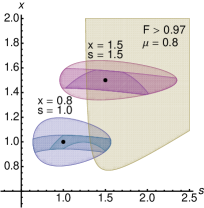
Figure 4: (Color online) (Left): subPoissonian region for $\rho_{G}$ states as a function of the purity $\mu$, the squeezing $s$, and the displacement $x$, together with the balloons of states having fidelity larger than $F_{G}>0.97$ to a nonclassical target with $\mu=0.9$, $s=1.4$, and $x=0.5$ and a classical one with $\mu=0.7$, $s=1.2$, and $x=1.5$. (Right): The subPoissonian region for a fixed value of purity $\mu=0.8$ as a function of squeezing and displacement, together with the balloons of states having fidelity larger than $F_{G}>0.97$ to the target states having $x=1.5$ and $s=1.5$ (subPoissonian) or $x=0.8$ and $s=1.0$ (superPoissonian). We also show the subregions of states having mean photon number and number fluctuations which differ at most $10\%$ from those of the target.

IV Two-mode Gaussian States

Here we focus on a relevant subclass of two-mode Gaussian states: the so-called two-mode squeezed thermal states (${\hbox{STS}_{2}}$) described by density operators of the form

$$\rho_{N\beta\gamma}=S_{2}(r)\nu(n_{1})\otimes\nu(n_{2})S_{2}^{\dagger}(r)$$ (12)

where $S_{2}(r)=\exp\{r(a^{\dagger}b^{\dagger}-ab)\}$ is the two-mode squeezing operator with real parameter $r$ and $\nu(n_{k})$, $k=1,2$ are thermal states with $n_{k}$ photon number on average. The class of states $\rho_{N\beta\gamma}$ is fully described by three parameters: the total mean photon number $N$, the two-mode squeezing fraction $\beta$ and the single-mode fraction of thermal photons: $\gamma$

$$\begin{split}&N=\langle a^{\dagger}a+b^{\dagger}b\rangle\\ &\beta=\frac{2\sinh^{2}r}{N}\\ &\gamma=\frac{n_{1}}{n_{1}+n_{2}}.\end{split}$$ (13)

The CM of ${\hbox{STS}_{2}}$ may be written in the block form

$$\sigma=\frac{1}{2}\begin{pmatrix}A\,\mathbb{I}&C\,\sigma_{z}\\ C\,\sigma_{z}&B\,\mathbb{I}\end{pmatrix}$$ (14)

with the coefficients parametrized according to (13):

$$\begin{split}A&=1+\frac{2\gamma(1-\beta)N+\beta N(1+N)}{1+\beta N}\\ B&=1+\frac{2(1-\gamma)(1-\beta)N+\beta N(1+N)}{1+\beta N}\\ C&=\frac{(1+N)\sqrt{\beta N(2+\beta N)}}{1+\beta N}.\end{split}$$ (15)

A squeezed thermal state is separable iff $\tilde{d}_{-}\geq\frac{1}{2}$, where $\sqrt{2}\tilde{d}_{\pm}=\sqrt{A^{2}+B^{2}+2C^{2}\pm(A+B)\sqrt{(A-B)^{2}+4C^{2}}}$ are the symplectic eigenvalues. Gaussian B-discord, i.e. the difference between the mutual information and the maximum amount of classical information obtainable by local Gaussian measurements on system B, may be analytically evaluated for ${\hbox{STS}_{2}}$ gd , leading to

$$D(\rho_{N\beta\gamma})=h(B)-h(d_{-})-h(d_{+})+h\left(\frac{A-C^{2}}{B+\frac{1}{2}}\right)$$ (16)

where $h(x)=(x+\frac{1}{2})\ln(x+\frac{1}{2})-(x-\frac{1}{2})\ln(x+\frac{1}{2})$. Finally, fidelity between two ${\hbox{STS}_{2}}$ is given by sorin ; Marian ; Oli12

$${F}_{N\beta\gamma}=\frac{(\sqrt{{X}}+\sqrt{{X}-1})^{2}}{\sqrt{\det[\sigma_{1}+\sigma_{2}]}}$$ (17)

where

$$X =2\sqrt{{E_{1}}}+2\sqrt{{E_{2}}}+\frac{1}{2}\,,$$

$$E_{1} =\frac{\det[\Omega\,\sigma_{1}\,\Omega\,\sigma_{2}]-\frac{1}{4}}{\det[\sigma_{1}+\sigma_{2}]}\,,$$

$$E_{2} =\frac{\det[\sigma_{1}+\frac{{\rm i}}{2}\Omega]\det[\sigma_{2}+\frac{{\rm i}}{2}\Omega]}{\det[\sigma_{1}+\sigma_{2}]}\,,$$

$\Omega$ being the $2$-mode symplectic form Oli12

$$\Omega=\omega\oplus\omega\qquad\omega=\left(\begin{array}[]{cc}0&1\\ -1&0\end{array}\right)\,.$$

In the left panel of Fig. 5 we show the separability region in terms of the three parameters $N$, $\beta$ and $\gamma$ together with the balloons of states having ${F}_{N\beta\gamma}>0.99$ with two target states: an entangled ${\hbox{STS}_{2}}$ with parameters $N=2.5$, $\beta=0.2$, $\gamma=0.5$ and a separable one with $N=1$, $\beta=0.13$ and $\gamma=0.5$. As it is apparent from the plot, both balloons cross the separability border and have a considerable overlap to both regions, thus making fidelity of little use to assess entanglement in these kind of systems.

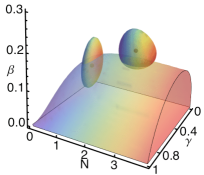
Figure 5: (Color online) (Left): Separability region of ${\hbox{STS}_{2}}$ in terms of the three parameters $N$, $\beta$ and $\gamma$ together with the balloons of states having ${F}_{N\beta\gamma}>0.99$ with two target states: an entangled ${\hbox{STS}_{2}}$ with parameters $N=2.5$, $\beta=0.2$, $\gamma=0.5$ and a separable one with $N=1$, $\beta=0.13$ and $\gamma=0.5$. (Right): the region of of states having a fidelity in the range $0.95<F_{N\beta\gamma}<0.99$ to a two-mode squeezed vacuum, $N=1$ and $\beta=1$. We also show the stripe of states having a mean photon number in the range $0.9<N<1.1$.

Another phenomenon arising from benchmarking with fidelity is illustrated in the right panel of Fig. 5, where we report the region of states having a fidelity in the range $0.95<F_{N\beta\gamma}<0.99$ to a two-mode squeezed vacuum, i.e. a maximally entangled state with $N=1$ and $\beta=1$. The emphasized sector corresponds to states that also have a mean photon number not differing more than $10\%$ from the target, i.e. in the range $0.9<N<1.1$. As a matter of fact, the total photon number $N$ and the squeezing fraction $\beta$ in this region may be considerably different from the targeted one and, in addition, the states with comparable energy are the least entangled in the region. Finally, in Fig. 6 we show the range of variation of Gaussian B-discord compatible with high values of fidelity. In the left panel we consider a non-separable target state with discord $D(\rho_{2,0.2,0.5})=0.22$ and a region of $\text{STS}_{2}$ states with fidelity $F_{N\beta\gamma}>0.95$. The region of separability (green) is crossed by a non negligible set of states and the relative variations of the discord is considerably large, ranging from $0.38$ to $1.88$. In the right panel of Fig. 6 we show again the wide range of variation of Gaussian B-discord for a set of $\text{STS}_{2}$ states with fidelity $0.95<F(\rho_{N\beta\gamma})<0.99$ to a target two-mode squeezed vacuum state with $N=2$. The high discrepancy in the relative discord can be only partially limited by constraining the mean photon number $N$ with fluctuations of the $10\%$. Notice that also in the case of two modes, full Gaussian tomography FullCM ; bla12 is imposing a suitable set of constraints to make fidelity a meaningful figure of merit to summarize the overall quality of the reconstruction.

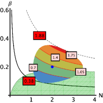
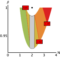
Figure 6: (Color online) (Left): Contour lines of Gaussian B-discord in the region of $\text{STS}_{2}$ having fidelity $F_{N\beta\gamma}>0.95$ to an entangled target state with $N=2,\beta=0.2$ and $\gamma=0.5$. The relative discord, rescaled to that of the target state ($D(\rho_{2,0.2,0.5})=0.22$), ranges from $0.38$ to $1.88$. (Right): Variations of the relative Gaussian B-discord in a region of $\text{STS}_{2}$ with fidelity $0.95<F_{N\beta\gamma}<0.99$ to a two-mode squeezed vacuum state ($N=2$ and $\beta=1$). In evidence the constrained region of states having the $10\%$ of energy fluctuations around $N=2$.

V Conclusions

In conclusion, we have shown by examples that being close in the Hilbert space may not imply being close in terms of quantum resources. In particular, we have provided quantitative examples for qubits and CV systems showing that pairs of states with high fidelity may include separable and entangled states, classical and nonclassical ones, and states with very different values of quantum of Gaussian discord.

Our results make apparent that in view of its wide use in quantum technology, fidelity is a quantity that should be employed with caution to assess quantum resources. In some cases it may be used in conjunction with additional constraints, whereas in the general situation it should be mostly used as an overall figure of merit, summarizing the findings of a full tomographic reconstruction.

- (1) A. Uhlmann, Rep. Math. Phys. 9, 273 (1976).
- (2) C. A. Fuchs, J. van de Graaf, IEEE Trans. Inf. Theory 45, 1216 (1999).
- (3) C. Benedetti, A. P. Shurupov, M. G. A. Paris, G. Brida, M. Genovese, Phys. Rev. A 87, 052136 (2013).
- (4) V. Dodonov, J. Phys. A 45, 032002 (2012).
- (5) S. Luo, Phys. Rev. A 77, 042303 (2008).
- (6) A. Miranowicz and A. Grudka, J. Opt. B 6, 542 (2004).
- (7) C. F. Roos, G. P. T. Lancaster, M. Riebe, H. Häffner, W. Hänsel, S. Gulde, C. Becher, J. Eschner, F. Schmidt-Kaler and R. Blatt, Phys. Rev. Lett. 92, 220402 (2004).
- (8) J.Fulconis, O. Alibart, J. L. O’Brien, W. J. Wadsworth and J. G. Rarity, Phys. Rev. Lett.99, 120501 (2007).
- (9) D. Riste, M. Dukalski, C. A. Watson, G. de Lange, M. J. Tiggelman, Ya. M. Blanter, K. W. Lehnert, R. N. Schouten, L. DiCarlo, Nature 502, 350 (2013).
- (10) L. Steffen, Y. Salathe, M. Oppliger, P. Kurpiers, M. Baur, C. Lang, C. Eichler, G. Puebla-Hellmann, A. Fedorov, A. Wallraff, Nature 500, 319 (2013).
- (11) C. T. Lee, Phys. Rev. A 44, R2775 (1991).
- (12) J Twamley, J. Phys. A 29, 3723 (1996).
- (13) H. Scutaru, J. Phys. A 31, 3659 (1998).
- (14) J. Řeháček, S. Olivares, D. Mogilevtsev, Z. Hradil, M. G. A. Paris, S. Fornaro, V. D’Auria, A. Porzio, S. Solimeno, Phys. Rev. A 79, 032111 (2009).
- (15) H. Paul, Rev. Mod. Phys. 54, 1061 (1982).
- (16) P. Giorda, M. G. A. Paris, Phys. Rev. Lett. 105, 020503 (2010).
- (17) Gh.-S. Paraoanu, H. Scutaru, Phys. Rev. A 61, 022306 (2000).
- (18) P. Marian, T. A. Marian, Phys. Rev. A 86, 022340 (2012).
- (19) S. Olivares, Eur. Phys. J. ST 203, 3 (2012).
- (20) V. D’Auria, S. Fornaro, A. Porzio, S. Solimeno, S. Olivares, M. G. A. Paris, Phys. Rev. Lett. 102, 020502 (2009); D. Buono, G. Nocerino, V. D’Auria, A. Porzio, S. Olivares, M. G. A. Paris, J. Opt. Soc. Am. B 27, 110 (2010).
- (21) R. Blandino, M. G. Genoni, J. Etesse, M. Barbieri, M. G. A. Paris, P. Grangier, R. Tualle-Brouri, Phys. Rev. Lett 109, 180402 (2012).