Kinematic Morphology of Large-scale Structure: Evolution from Potential to Rotational Flow

Abstract

As an alternative way of describing the cosmological velocity field, we discuss the evolution of rotational invariants constructed from the velocity gradient tensor. Compared with the traditional divergence-vorticity decomposition, these invariants, defined as coefficients of characteristic equation of the velocity gradient tensor, enable a complete classification of all possible flow patterns in the dark-matter comoving frame, including both potential and vortical flows. We show that this tool, first introduced in turbulence two decades ago, proves to be very useful in understanding the evolution of the cosmic web structure, and in classifying its morphology. Before shell-crossing, different categories of potential flow are highly associated with cosmic web structure, because of the coherent evolution of density and velocity. This correspondence is even preserved at some level when vorticity is generated after shell-crossing. The evolution from the potential to vortical flow can be traced continuously by these invariants. With the help of this tool, we show that the vorticity is generated in a particular way that is highly correlated with the large-scale structure. This includes a distinct spatial distribution and different types of alignment between cosmic web and vorticity direction for various vortical flows. Incorporating shell-crossing into closed dynamical systems is highly non-trivial, but we propose a possible statistical explanation for some of these phenomena relating to the internal structure of the three-dimensional invariants space.

1. Introduction

The peculiar velocity $\mathbf{u}$, together with the density distribution $\rho$ of dark matter, encode abundant information about the evolution of large-scale structure of our Universe. Besides its statistical manifestation via redshift-space distortions (Kaiser, 1987; Davis & Peebles, 1983; Hamilton, 1992; Cole et al., 1994), the line-of-sight component of the peculiar flow of individual galaxies can also be obtained from distance indicators such as the Tully-Fisher relation (Tully & Fisher, 1977) between galaxy luminosity and rotational velocity, and the transverse component from the proper motion of galaxies (Nusser et al., 2012) by highly accurate astrometric experiments like Gaia. Such a dataset of large-scale three-dimensional peculiar velocities would provide valuable information for our theory of the evolution of dark matter velocity field.

A virtue of three-dimensional velocity data is the ability to study the vorticity contribution $\mathbf{w}=\nabla\times\mathbf{u}$ (Peebles, 1980; Pueblas & Scoccimarro, 2009; Hahn et al., 2014), which in the standard cosmology model is negligible on large scale and is mainly generated after the shell-crossing at later epoch, since any initial rotational component will decay rapidly due to the expansion of the Universe. And for a long time, the divergence contribution $\theta=\nabla\cdot\mathbf{u}$, as the only remaining degree of freedom of $\mathbf{u}$, dominates most of raw theoretical as well as observational investigations in this field. However, in the nonlinear regime, the vectorial rotational component might contain valuable morphological information that is lost if only the divergence is studied. To learn more about the cosmic flow in detail, in this paper we are interested in the gradient tensor of the velocity field $\mathbf{u}$,

$$A_{ij}(\mathbf{x},\tau)=\frac{\partial u_{i}}{\partial x_{j}}(\mathbf{x},\tau)$$ (1)

where $\mathbf{x}$ is Eulerian position and $\tau$ the comoving time.

The tensor $A_{ij}$ is closely related with cosmic web structure, since it characterizes the velocity variations around a mass element as it moves away from a void or toward halo/filamentary/wall structures. For irrotational flow, $\mathbf{u}=-\nabla\psi$ where $\psi$ is the velocity potential. At the linear order, $\psi$ is proportional to the gravitational potential $\Phi$; therefore, the tensor $A_{ij}\approx\nabla_{i}\nabla_{j}\Phi$ encodes information about the anisotropic gravitational field, which eventually leads to the formation of the cosmic web structure. Given the importance of cosmic web in understanding large-scale structure formation (Bond et al., 1996), many techniques have been developed to classify cosmic web in numerical simulation (Pogosyan et al., 2009; Aragon-Calvo et al., 2010; Sousbie, 2011a, b; Bond et al., 2010; Forero-Romero et al., 2009; Hahn et al., 2007a; Sousbie et al., 2009; Stoica et al., 2005). Similar to the method using the tidal field, or equivalently the Hessian matrix of density, one usually considers the eigenvalues $\lambda_{i}$ of tensor $A_{ij}$. Neglecting the subtleties in selecting the criteria, in general, entirely positive/negative eigenvalues correspond to an entirely stretching/compressing region, i.e. a void/halo, and a matrix with both positive and negative eigenvalues gives wall or filament structures, e.g. Hoffman et al. (2012). However, besides its implicit coordinate system dependence, once the vorticity is generated, the anti-symmetric tensor $A_{ij}$ gives complex eigenvalues $\lambda_{i}$, and therefore complicates the discussion of flow morphology in such language.

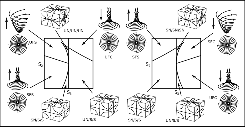
Figure 1.— Illustration of various cosmic flow types in invariants space. We only show 2D $s_{3}-s_{2}$ plane with fixed $s_{1}$; the left panel shows negative $s_{1}$, and the right panel shows positive $s_{1}$.

In this paper, we consider an alternative way of describing flow morphologies, as well as its applications. To eliminate coordinate dependence, one would prefer the scalar fields that are rotational invariants built from the velocity gradient tensor $A_{ij}$. The eigenvalue problem of tensor $A_{ij}$ is given by

$$\det[A_{ij}-\lambda\delta_{ij}]=\lambda^{3}+s_{1}\lambda^{2}+s_{2}\lambda+s_{3}=0,$$ (2)

where $\delta_{ij}$ is identity matrix. The coefficients $s_{i}$, where $i=\{1,2,3\}$, appearing in Eq. (2), are natural quantities to study. For various irrotational flows that have been discussed, the criteria in eigenvalue space are then mapped into different regions in the invariants space (Chong et al., 1990). One advantage of working in this parameter space is to avoid the complex domain after the emergence of vorticity and $A_{ij}$ becoming anti-symmetric. It enables one to continuously explore the evolution from potential to vortical flow in a uniform framework.

Furthermore, compared with rotation dependent matrix $A_{ij}$, these invariants are also appropriate device for analytical study of the dynamical evolution of the cosmic flow. Starting from initial fluctuations with negligible rotational degrees of freedom, one is able to trace in the invariants space the evolution of kinematic morphologies of a dark matter element as it travels away from an underdense region toward filaments or halos, eventually experiencing various types of vorticity in the multi-streaming regime. However, analytical study of the growth of vorticity is highly non-trivial (Pueblas & Scoccimarro, 2009), since it mainly occurs at non-linear small scale which beyond the reach of approaches like perturbation theory. And the efforts to incorporate the shell-crossing would result in a hierarchy of fluid dynamical equations that would need to be closed. One approach is to model or measure the velocity dispersion and truncate the hierarchy (e.g.  Pueblas & Scoccimarro, 2009). In this paper, as suggested by our numerical measurement of vortical morphologies, the stochasticity of the process may provide some new insight.

Even for the collapsed objects like halos, the full information of tensor $A_{ij}$ is important. Theoretically the angular momentum of halo is largely explained by the tidal torque theory (Hoyle, 1949; Peebles, 1969; Doroshkevich, 1970; White, 1984; Wesson, 1985), which explains the formation of halo spin from laminar flow by the misalignment between shear and inertia, and it predicts a linear growth of angular momentum. But this mechanism is only effective prior to turn-around in the spherical-collapse picture; after this, the collapse dramatically reduces the lever arm (Schafer, 2009), and the alignment between halo spin and vorticity direction found by Libeskind et al. (2013a) suggests a separate phase of the growth of halo angular momentum. The coevolution picture between halo spin and vorticity supports our finding from invariants, because investigations using $N$-body simulations also indicate the existence of preferential orientation between halo spin and filaments (Hahn et al., 2007a; Sousbie et al., 2009; Zhang et al., 2009; Laigle et al., 2013; Dubois et al., 2014; Aragon-Calvo & Yang, 2014). Indeed, several authors have found mass-dependent alignment of halo spins with filaments; low-mass halos tend to be aligned with filaments, and high-mass halos have spin perpendicular to the filaments (Aragon-Calvo et al., 2007; Hahn et al., 2007b; Paz et al., 2008; Sousbie et al., 2009; Codis et al., 2012; Aragon-Calvo, 2013). In fact, Tempel & Libeskind (2014) have found evidence for this alignment in SDSS galaxies.

The purposes of this paper are severalfold. After introducing the invariants of the velocity gradient tensor at the beginning of section II., we show its ability to classify flow morphologies for both potential and vortical flow, and then discuss the connection to the cosmic web structure. Then we try to investigate the dynamical evolution of these invariants, first for irrotational flow in section III., and then in section IV. study the emergence of vorticity through shell-crossing. For simplicity, after deriving the full dynamical equations before shell-crossing, we first study the Zel’dovich approximation, obtaining the exact numerical solution as well as the probability distribution of invariants. In section IV., we first present the result relating to the vorticity measured from N-body simulation, and then setup both the dynamical and statistical view for physical interpretation. Finally, we discuss and conclude in section V.

Throughout the paper, we make our numerical measurement with two different sets of $N$-body simulations. For the purpose of irrotational flow only, we use a simulation with box size $100h^{-1}{\rm Mpc}$ and $512^{3}$ particles, hereafter we will denote as ‘$Sing100$’. However the spatial resolution is not high enough to study vortical flow which are generated at very small scale. To achieve a clean signal with high signal-to-noise ratio and meanwhile explore the relation to large-scale structure, we use the MIP (Multum In Parvo, ‘many things in the same place’) ensemble simulation (Aragon-Calvo, 2012), which is a suite of $N$-body simulations constrained to have the same large-scale structure for initial Fourier modes with wavelengths over $4h^{-1}{\rm Mpc}$, but independent small scale realizations. The combining of many realizations enables one to visually inspect the correspondence between rotational flow and cosmic-web. The ensemble has $256$ realizations of a $32h^{-1}{\rm Mpc}$ box with $256^{3}$ particles each. This is equivalent in terms of effective volume and number of particles to a box of $193~{}h^{-1}{\rm Mpc}$ of side with $\sim 1540^{3}$ particles containing $\sim 5\times 10^{6}$ haloes with a minimum mass of $3.25\times 10^{9}h^{-1}M_{\odot}$. To numerically estimate the spatial gradient $A_{ij}$, we first construct the velocity field on a regular Eulerian grid with Delaunay tessellation (Bernardeau & van de Weygaert, 1996; Pueblas & Scoccimarro, 2009; Schaap & van de Weygaert, 2000; Pelupessy et al., 2003), and then take the gradient in real space. Although this method is known to have a better noise property in measuring velocity divergence and vorticity (Pueblas & Scoccimarro, 2009), it still implicitly involves coarse-graining and is less accurate than more sophisticated method with explicit phase space projection (Hahn et al., 2014).

2. Invariants of Velocity Gradient Tensor and Local Flow Morphology

The invariants of the velocity gradient tensor have been studied in turbulence for more than two decades since their introduction by Chong et al. (1990). They describe fundamental and intrinsic properties of small-scale motions in turbulence (Meneveau, 2011). In this section, we will first present the definition of the invariants of the velocity gradient tensor, discuss their ability to classify various potential and rotational flow morphologies, and then show the connection with cosmic web structure.

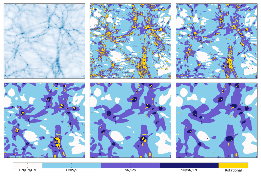
Figure 2.— Various classifications of cosmic flow with different degrees of smoothing, compared with the un-smoothed density field (first panel) of the same snapshot of simulation ‘$Sing100$’ at redshift $z=0$. The box size is $100{\rm Mpc}/h$. Various categories are labeled as their kinematical morphologies, the definitions are discussed in Sec. 2.2 (also see Fig. 1). Starting from the second panel, we use Gaussian smoothing scales $R=0.2{\rm Mpc}/h,~{}0.4{\rm Mpc}/h,~{}0.8{\rm Mpc}/h,~{}1.2{\rm Mpc}/h$ and $1.5{\rm Mpc}/h$. The rotational region is suppressed increasingly for larger smoothing length.

2.1. Definition of Invariants

Among all nine elements in tensor $A_{ij}$, six degrees of freedom are rotationally invariant, and the other three encode coordinate information. As discussed in the introduction, to extract the morphological information, we are particularly interested in the coefficients of the characteristic equation $\det[\mathbf{A}-\lambda I]=0$, i.e.

$$\lambda^{3}+s_{1}\lambda^{2}+s_{2}\lambda+s_{3}=0,$$ (3)

where the invariants $s_{1},s_{2},s_{3}$ are defined as (Chong et al., 1990)

$$s_{1} = -\rm tr[\mathbf{A}]=-\theta_{ii},$$

$$s_{2} = \frac{1}{2}\left(s_{1}^{2}-\rm tr[\mathbf{A}^{2}]\right)=\frac{1}{2}(s_{1}^{2}-\theta_{ij}\theta_{ji}-\omega_{ij}\omega_{ji})$$

$$s_{3} = -\det[\mathbf{A}]=\frac{1}{3}\left(-s_{1}^{3}+3s_{1}s_{2}-\rm tr[\mathbf{A}^{3}]\right)$$ (4)

$$= \frac{1}{3}\left(-s_{1}^{3}+3s_{1}s_{2}-\theta_{ij}\theta_{jk}\theta_{ki}-3\omega_{ij}\omega_{jk}\theta_{ki}\right).$$

Here we have decomposed $A_{ij}$ into a symmetric part $\theta_{ij}$ and an anti-symmetric part $\omega_{ij}$,

$$A_{ij}=A_{(ij)}+A_{[ij]}=\theta_{ij}+\omega_{ij},$$ (5)

where

$$\theta_{ij}=\frac{1}{2}(A_{ij}+A_{ji}),\qquad\omega_{ij}=\frac{1}{2}(A_{ij}-A_{ji}).$$ (6)

The tensor $\theta_{ij}$ denotes the rate of deformation of a fluid element and $\omega_{ij}$ the rate of rotation, which relates to the vorticity vector $\omega_{i}$ through $\omega_{i}=-\epsilon_{ijk}\omega_{jk}$, where $\epsilon_{ijk}$ is the totally anti-symmetric Levi-Civita symbol. To better understand the physics of these invariants $s_{i}$, we could further decompose the rate of deformation into isotropic and anisotropic part, i.e. the divergence $\theta$ and the shear tensor $\sigma_{ij}$

$$\theta_{ij}=\sigma_{ij}+\frac{1}{3}\theta\delta^{K}_{ij},$$ (7)

where $\delta^{K}_{ij}$ is the Kronecker delta, and also define the magnitude of tensor $\sigma_{ij}$ and $\omega_{ij}$ as

$$\sigma=\left(\frac{1}{2}\sigma_{ij}\sigma_{ij}\right)^{1/2},\qquad\omega=\left(\frac{1}{2}\omega_{ij}\omega_{ij}\right)^{1/2}.$$ (8)

With the above definitions, the invariants we just introduced can be expressed as

$$s_{1} = -\theta$$

$$s_{2} = \frac{1}{3}\theta^{2}-\sigma^{2}+\omega^{2}$$

$$s_{3} = -\frac{1}{27}\theta^{3}+\frac{1}{3}\theta\left(\sigma^{2}-\omega^{2}\right)-\frac{1}{3}\sigma_{ij}\sigma_{jk}\sigma_{ki}-\frac{1}{4}\sigma_{ij}\omega_{i}\omega_{j}.$$

In turbulence, many studies concentrate on incompressible flow at $\theta=0$, invariants $s_{2}=\omega^{2}-\sigma^{2}$ and $s_{3}=-\sigma_{ij}(\sigma_{jk}\sigma_{ki}/3+\omega_{jk}\omega_{ki})$ then describe the balance only between the shearing $\sigma_{ij}$ and vorticity $\omega_{ij}$. It is then reasonable to discuss these two contributions separately, and therefore one could define remaining scalar degree of freedom of $A_{ij}$ as, e.g. the symmetric $s^{(s)}_{i}$ (or anti-symmetric $s^{(a)}_{i}$) contribution to $s_{2}$ and $s_{3}$, where

$$s_{i}=s^{(s)}_{i}+s^{(a)}_{i},\qquad i=(2,3).$$ (10)

In cosmology, however, $\theta$ is in general nonzero, the anti-symmetric contribution could be expressed as

$$s^{(a)}_{2} = -\frac{1}{2}\omega_{ij}\omega_{ji}=\omega^{2},$$

$$s^{(a)}_{3} = s_{1}s^{(a)}_{2}-\omega_{ij}\omega_{jk}\theta_{ki}$$ (11)

$$= -\frac{1}{3}\theta\omega^{2}-\frac{1}{4}\sigma_{ij}\omega_{i}\omega_{j}.$$

As will be seen later, before shell-crossing, $s^{(a)}_{2}$ and $s^{(a)}_{3}$ vanish, eigenvalues $\lambda_{i}$ of matrix $A_{ij}$ and therefore the local cosmic web are entirely determined by $s^{(s)}_{i}(i=1,2,3)$. Once the vorticity is generated after shell-crossing, it will then couple to symmetric contribution, via $s^{(a)}_{i}$, and affect morphological classification of the local flow. Therefore, the generation of rotational flow is much more complicated, not merely related to vorticity. Moreover, since $\omega_{ij}$ contributes to both $s_{2}$ and $s_{3}$, it is possible to generate laminar flow with non-zero vorticity (Appendix B).

2.2. Classification of the Local Flow

As they are the coefficients of the characteristic equation, the most direct application of $s_{i}$ is the classification of the solutions $\lambda_{i}$. The trajectory around a given point $\mathbf{x}_{0}$ can be approximated with a Taylor expansion,

$$\frac{dx_{i}}{d\tau}(\mathbf{x})=u_{i}(\mathbf{x})=u_{i}(\mathbf{x}_{0})+A_{ij}(\mathbf{x}_{0})x_{j}+\cdots$$ (12)

In the dark-matter comoving frame where $u_{i}(\mathbf{x}_{0})=0$, ignoring higher-order terms, one obtains the local trajectory of a fluid element via the differential equation

$$\frac{dx_{i}}{d\tau}=A_{ij}x_{j}.$$ (13)

Therefore to first order, $\mathbf{A}$ characterizes the local trajectory of the fluid element. As will be shown later, neglecting the rotational degree of freedom of the coordinate system, various flow morphologies presented by solving Eq. (13) in the canonical form of $\mathbf{A}$ can be mapped into invariants space. Therefore, the three-dimensional real parameter space is then divided into various adjacent regions. Among them, the most important criteria is the surface dividing the real and complex roots of $\lambda_{i}$, which is defined by the equation

$$27s_{3}^{2}+(4s_{1}^{3}-18s_{1}s_{2})s_{3}+(4s_{2}^{3}-s_{1}^{2}s_{2}^{2})=0$$ (14)

Using the discriminant $s_{2}\leq s_{1}^{2}/3$ of the above quadratic equation, one is able to define real solutions of $s_{3}$, which we will denote as $s_{3a}$ and $s_{3b}$, assuming $s_{3a}\leq s_{3b}$. For real eigenvalues, the inequality $s_{3a}\leq s_{3}\leq s_{3b}$ should hold, or there will be complex eigenvalues otherwise.

In the following of this section, we will review the work of Chong et al. (1990), and show how different flow morphologies could be classified according to the eigenvalues of $A_{ij}$ and its image in the invariants space. Here, we only discuss the most relevant categories in a cosmological context. A more complete classification including all degenerating special cases could be found in the original paper. For convenience, in the Appendix A., we also give a list of categories have been discussed, correcting some typos in Chong et al. (1990).

As will be seen later, the discussion of flow morphology is possible only in an appropriate coordinate system. For potential flow, $A_{ij}$ is symmetric, and therefore could always be diagonalized over the field of real numbers.

$$\mathbf{A}=\mathbf{R}^{-1}\left(\begin{array}[]{ccc}\lambda_{1}&&\\ &\lambda_{2}&\\ &&\lambda_{3}\\ \end{array}\right)\mathbf{R},\qquad\lambda_{i}\in\mathbb{R}$$ (18)

where $\mathbf{R}$ is a rotation matrix and we assume $\lambda_{1}\leq\lambda_{2}\leq\lambda_{3}$. From Eq. (18) and the definition of $s_{i}$, the invariants can simply be expressed as

$$s_{1}=-\sum_{i}\lambda_{i},\quad s_{2}=\sum_{i\neq j}\lambda_{i}\lambda_{j},\quad s_{3}=-\prod_{i}\lambda_{i}.$$ (19)

For a general anti-symmetric matrix $\mathbf{A}$, although in many cases Eq. (18) and (19) are still valid over complex field $\lambda_{i}\in\mathbb{C}$, it is not easy to extract geometric information out. Therefore, it is more convenient to rotate the matrix into a well-suited frame as described in Sec 2.2.2. In some situations, $\mathbf{A}$ is not diagonalizable. However, these are very special cases and are unlikely to be important in cosmological context.

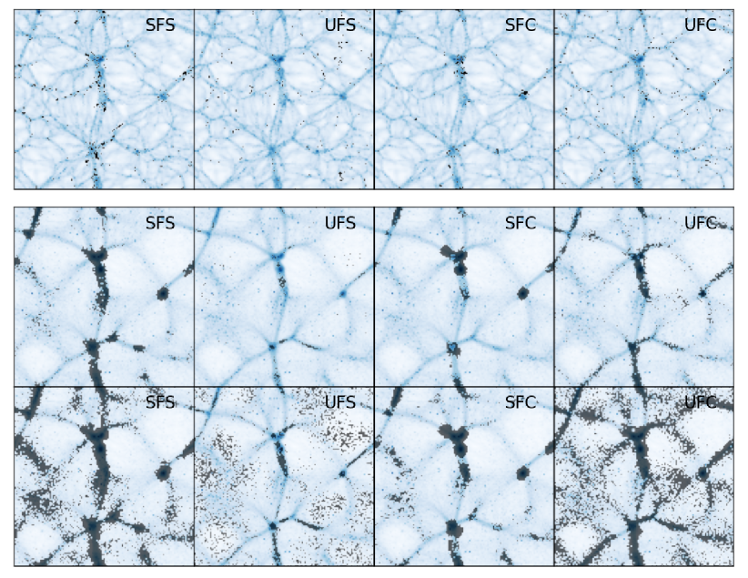
Figure 3.— Four different categories of vortical flow in the MIP ensemble, a suite of simulations with the same large-scale structure but independent small-scale realizations. Every column presents the same morphologies labeled in the upper-right corner of each panel. The top row makes use of only one realization, and therefore show very small fractions of the region are classified as rotational categories, which is reasonable given the resolution of our simulation. To display more clearly the spatial distribution of various rotational categories, we utilize the whole ensemble simulation in the middle and bottom rows, where much larger area highlights the region where more than $n_{ct}$ out of $64$ realizations are labeled as a particular rotational category. We adopt $n_{ct}=5$ for the middle row and $2$ for the bottom. The density field of these two are also stacked over all realizations, and that is the reason why small-scale structures are smeared out.

2.2.1 Potential Flow

For potential flow, our method categorizes different morphologies according to the sign of eigenvalues of $A_{ij}$ or corresponding regions in the invariants space. In this regime, many similar algorithms have already been proposed to use either the Hessian matrix of gravitational potential $\nabla_{i}\nabla_{j}\Phi$ (Hahn et al., 2007a; Forero-Romero et al., 2009) or similar to our method, the symmetric part of $A_{ij}$ (‘V-web’, Hoffman et al., 2012). Instead of introducing a free parameter of the threshold eigenvalues $\lambda_{th}$, which is usually adjusted to match the visual impression (Hoffman et al., 2012), our method simply sets $\lambda_{th}=0$. However, it is not difficult to incorporate this parameter explicitly. One just defines $\lambda^{\prime}=\lambda-\lambda_{th}$ and rewrites the characteristic equation (3) as a function of $\lambda^{\prime}$,

$$(\lambda^{\prime}+\lambda_{th})^{3}+s_{1}(\lambda^{\prime}+\lambda_{th})^{2}+s_{2}(\lambda^{\prime}+\lambda_{th})+s_{3}=0,$$ (20)

then discusses the sign of variable $\lambda^{\prime}$ instead. Expanding Eq. (20), this is equivalent to defining a new set of invariants $s^{th}$,

$$s^{th}_{1} = s_{1}+3\lambda_{th}$$

$$s^{th}_{2} = s_{2}+2\lambda_{th}s_{1}+3\lambda_{th}^{2}$$

$$s^{th}_{3} = s_{3}+\lambda_{th}s_{2}+\lambda_{th}^{2}s_{1}+\lambda_{th}^{3}.$$ (21)

Then all classification conditions of the invariants that will be introduced in the following remain the same.

Since the symmetric matrix $A_{ij}$ can be diagonalized into canonical form (18), there will exist three eigen-planes, that contain solution trajectories. These trajectories may look like nodes and saddles on the plane , depending on the sign of the eigenvalues. Particularly when all eigenvalues $\lambda_{i}<0$, then three planes contain nodes. So the mass elements would all flow toward the position of interest $\mathbf{x}_{0}$ in each eigen-planes, which is more likely to occur in the over-dense region, around halos. The mapping from $\lambda_{i}<0$ in eigenvalue space into invariants space is straightforward, since from Eq. (19), we see $s_{i}>0$ for all $i=(1,2,3)$. Combined with the real solution condition (Eq. A3), this type corresponds to a region in invariants space,

$$s_{1}>0,~{}0<s_{2}<s_{1}^{2}/3,~{}\max(s_{3a},0)<s_{3}<s_{3b}.~{}$$ (22)

As illustrated in Fig. (1), the streamlines in this region are all ‘stable nodes’ in all three eigen-planes, and therefore it will be denoted as ‘$\mathcal{SN/SN/SN}$’ in the following.

On the other hand, when all eigenvalues $\lambda_{i}>0$, one still gets three nodes, but the flow will all head outward from the origin, which most likely would happen in under-dense region, in the void. Similarly from Eq. (19), $s_{1},s_{3}<0$ and $s_{2}>0$, and with real root condition, it corresponds to region in invariants space

$$s_{1}<0,~{}0<s_{2}<s_{1}^{2}/3,~{}s_{3a}<s_{3}<\min(s_{3b},0).~{}$$ (23)

And we will denote this type as ‘$\mathcal{UN/UN/UN}$’ where ‘$\mathcal{UN}$’ stands for ‘unstable node’.

If the matrix $A_{ij}$ becomes indefinite, i.e. with both positive and negative eigenvalues, then it possess saddle points in two eigenvector planes. As shown in Fig. (1), in the eigen-plane with saddle point, the flow will approach inward from one direction and depart toward the other without passing through the origin. Particularly when the smallest two eigenvalues $\lambda_{1},\lambda_{2}$ are negative, while $\lambda_{3}$ positive, two saddle points reside in the planes spanned by $\mathbf{v}_{1}-\mathbf{v}_{3}$ and $\mathbf{v}_{2}-\mathbf{v}_{3}$, where $\mathbf{v}_{i}$ is the eigenvector corresponding to $\lambda_{i}$, and the node in plane $\mathbf{v}_{1}-\mathbf{v}_{2}$ is stable, i.e. mass elements flow inward. Therefore, we will name this category as ‘$\mathcal{SN/S/S}$’, where the last two ‘$\mathcal{S}$’ denote ‘saddle point’. From the illustration of the trajectory in Fig. (1), this type resembles the situation when the mass element flow along the filamentary structures. In invariants space, the sum of $\lambda_{i}$ could be either positive or negative depending on the relation between $|\lambda_{1}+\lambda_{2}|$ and $\lambda_{3}$. If $s_{1}\geq 0$, i.e. $|\lambda_{1}+\lambda_{2}|\geq\lambda_{3}$, the flow changes faster in the node plane $\mathbf{v}_{1}-\mathbf{v}_{2}$, and causes the net compression of the fluid element. While if $s_{1}<0$, it happens the opposite way. In summary, we have

$$~{}~{}s_{1}\geq 0,\qquad s_{2}<s_{1}^{2}/4,\qquad s_{3a}<s_{3}<0,$$

$$or ~{}~{}s_{1}<0,\qquad s_{2}<0,\qquad s_{3a}<s_{3}<0.$$ (24)

When only the smallest eigenvalue $\lambda_{1}$ is negative, and $\lambda_{2},\lambda_{3}$ positive, then two saddle points reside in the planes spanned by $\mathbf{v}_{1}-\mathbf{v}_{2}$ and $\mathbf{v}_{1}-\mathbf{v}_{3}$, and the node in the plane $\mathbf{v}_{2}-\mathbf{v}_{3}$ is unstable since $\lambda_{2,3}>0$. This corresponds to the case when matter flow towards a wall structure. Again in the invariants space, we’ll also have two conditions

$$~{}~{}s_{1}\leq 0,\qquad s_{2}<s_{1}^{2}/4,\qquad 0<s_{3}<s_{3b},$$

$$or ~{}~{}s_{1}>0,\qquad s_{2}<0,\qquad 0<s_{3}<s_{3b}.$$ (25)

Similarly, $s_{1}\leq 0$ corresponds to faster velocity change in the node plane $\mathbf{v}_{2}-\mathbf{v}_{3}$, and a net expansion of the fluid element. If $s_{1}>0$, the fluid element contracts.

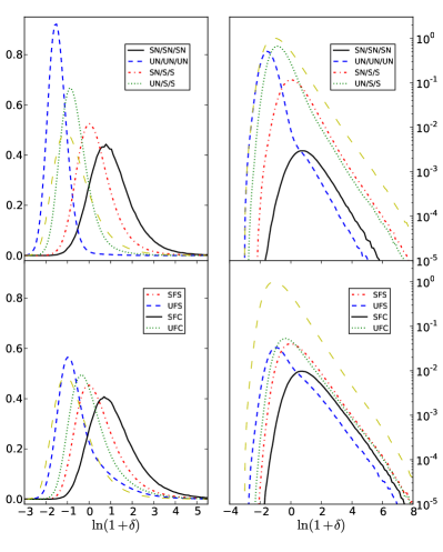
Figure 4.— Left: the PDF of density $1+\delta$ for various flow morphologies, drawn from the ‘$Sing100$’ simulation. Right: same as left panels but all curves have been rescaled by the volume fraction of each morphology type, so that the maxima of entire density field (long-dashed line) equal unity. Upper: distribution of various potential flow. Lower: distribution of rotational flow.

2.2.2 Vortical Flow

After shell crossing, the anti-symmetric part $\omega_{ij}$ of the matrix $A_{ij}$ will be generated. In terms of real numbers, the canonical form of $A_{ij}$ can be expressed as

$$\mathbf{A}=\mathbf{R}^{-1}\left(\begin{array}[]{ccc}a&-b&\\ b&a&\\ &&c\\ \end{array}\right)\mathbf{R},$$ (29)

where $a,b,c$ are all real, and the complex eigenvalue $\lambda_{1,2}=a\pm ib$, $\lambda_{3}=c$. Then the invariants simply read as

$$s_{1}=-(2a+c),\quad s_{2}=a^{2}+b^{2}+2ac,$$

$$s_{3}=-c(a^{2}+b^{2}).\qquad\qquad\quad$$ (30)

In this case, there will exist one plane, corresponding to eigenvalues $\lambda_{1,2}$, that contains the solution trajectory, which can be expressed as

$$r=r_{0}e^{m\alpha}$$ (31)

in polar coordinates $(r,\alpha)$. Here the factor $m=a/b$ denotes the rate of spiraling, and $r_{0}$ is a constant depending on the initial condition. Along the direction of $\lambda_{3}$, the behavior of the trajectory is then controlled by the value of $c$.

Depending on the value of $m$ and $c$, and neglecting degenerate cases, there remain four major categories of rotational flow. For negative $m$, the trajectory spirals inwards to the origin of the plane, which will be called ‘stable focal flow’ in the following. If $c>0$, mass elements flow away from the plane, a situation denoted ‘$\mathcal{SFS}$’, i.e. ‘stable focal stretching.’ If $c<0$, mass elements flow towards the plane, and we will call it as ‘stable focal compressing’, abbreviated as ‘$\mathcal{SFC}$’. For positive $m$, the trajectory spirals outwards from the origin, and the flow is called ‘unstable focal flow’. Depending on the value of $c$, the last two flow types are called ‘unstable focal stretching’, abbreviated as ‘$\mathcal{UFS}$’ for $m>0,c>0$; ‘unstable focal compressing’, abbreviated as ‘$\mathcal{UFC}$’ for $m>0,c<0$. The detailed criteria for vortical regions are listed in Appendix A.

2.3. Cosmic Web and Kinematic Morphologies

To show the relationship between large-scale-structure morphologies and the kinematic classification, we highlight different categories of flow patterns of ‘$Sing100$’ simulation at redshift $z=0$ and compare with the density field in Fig. (2). Since the process of cosmic web formation is largely associated with potential flow, and to avoid disturbance from rotational degree of freedom, we smooth the velocity field with a Gaussian filter with smoothing length varying from $R=0.2{\rm Mpc}/h$ to $1.5{\rm Mpc}/h$. Notice that different categories are labeled by their kinematic names such as ‘$\mathcal{SN/SN/SN}$’, instead of the more familiar ‘halo’, since by setting $\lambda_{th}=0$, our morphology classification does not necessarily reproduce the best visual structures compared with ‘V-web’ (Hoffman et al., 2012). Since our method includes both potential and rotational morphologies, cosmic-web structures, especially filaments, defined with irrotational flow could only be identified with relative large smoothing length. However, with an appropriate smoothing, e.g. $R=0.8{\rm Mpc}/h$ as shown in the lower left panel, one does see a good visual correspondence between filamentary cosmic web in the density (first panel) and the corresponding kinematic categories ‘$\mathcal{SN/SN/SN}$’ (halo-like) and ‘$\mathcal{SN/S/S}$’ (filament-like). This mainly reflects the connection between the velocity potential $\psi$ and gravitational potential $\Phi$ on large scales. As one performs the smoothing more aggressively, features at small scale vanish as expected. However, unlike the wall/sheet structure identified in Hoffman et al. (2012), our wall-like ‘$\mathcal{UN/S/S}$’ type fills almost half of the simulation volume. Although more studies are desired, we tend to believe this is a combined effect of both the larger Eulerian volume filling factor for underdense regions and the relative larger volume in the invariants space, as could be seen in Fig. (1). From Fig. (2), we could also see that the large-scale structure identified kinematically is reliable with various degree of smoothing, although the rotational categories, shown in yellow, is reduced dramatically as one increases the smoothing length.

To better understand these rotational regions in Fig. (2), we use the MIP $N$-body ensemble simulations and show the spatial distribution of four vortical flow categories in Fig. (3). One benefit of using the MIP simulation is that, since vorticity is only generated at small scales after shell-crossing, in a single realization of a moderate resolution simulation, one will not have many pixels classified as rotational. Moreover, because the classification criteria is mutually exclusive, each pixel can only be categorized as one of them. On the other hand, with the full suite of MIP simulation, one can explore the ensemble probability of generating one particular morphology given the large-scale environment. For this purpose, we first make a complete classification of all realizations, and then highlight the region where more than $n_{ct}$ out of $64$ are categorized as a certain type. By doing this, each pixel of the simulation could be multi-valued. The result is shown in Fig. (3), where the first row illustrate the vortical classification of an arbitrary realization while the middle and bottom row are combined classification with $n_{ct}=5$ and $2$ respectively. The underlying density distribution of the last two rows are produced by stacking all $64$ realizations, therefore lacking the small-scale structure compared with the first. Similar to the irrotational morphologies, the most distinctive feature of the figure is that various flow categories display different spatial distributions. For example, ‘$\mathcal{SFC}$’ resides around knots and ‘$\mathcal{SFS}$’ and ‘$\mathcal{UFC}$’ are located along filaments; this is especially clear for lower $n_{ct}$. Furthermore, as we will discuss further below, the direction of the vorticity of different categories also vary among different categories.

Besides the spatial distribution, we also plot in Fig. (4) the probability density function (PDF) of matter density for various irrotational flow categories in the upper panels and vortical types in the lower. While the PDF is displayed at left, we also present curves rescaled by the volume fraction of each morphology type at right. From left panels, one notices the locations of PDF maxima of each category in $(1+\delta)$-axis, $\delta_{max}$, exhibit a sequence consistent with their cosmic web morphologies. That is, the PDF of type ‘$\mathcal{SN/SN/SN}$’ peaks at higher density value $\delta$ than that of type ‘$\mathcal{SN/S/S}$’; we identify these as halo and filament respectively; following these are wall/sheet and void types. On the other hand, as shown in the lower panel, $\delta_{max}$ of vortical types are all greater than that of the entire field (long-dashed line), which is reasonable since they are only generated after shell-crossing in denser regions. Although the differences of peak positions among all vortical categories are narrower than for potential types, they are still consistent with the spatial distribution from Fig(̇3): the type ‘$\mathcal{SFS}$’ around knots are highest-density, then follow ‘$\mathcal{SFS}$’ and ‘$\mathcal{UFC}$’, which trace filaments. From the right panels, one could further see the relative volume abundance of each category. Since the distributions are volume weighted in Eulerian space, higher density regions are expected to be less abundant. This explains the lower amplitude of category ‘$\mathcal{SN/SN/SN}$’ and ‘$\mathcal{SFC}$’ in the figure. Also, as consistent with the visual impression of Fig. (2), more regions are classified as ‘$\mathcal{UN/S/S}$’ instead of ‘$\mathcal{UN/UN/UN}$’.

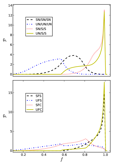
Figure 5.— The fractional anisotropy defined in Eq. (32) for various flow morphologies from ‘$Sing100$’ simulation. Upper: Potential flows; lower: rotational flows.

To further examine our invariants-based cosmic web classification, we also investigate the isotropy of each category, since to some level halos and voids should be more isotropic than filaments and walls. For the same purpose, Libeskind et al. (2013b) measured the fractional anisotropy for their shear based ‘V-web’ classification,

$$f_{a}=\frac{1}{\sqrt{3}}\sqrt{\frac{\sum_{i<j}(\lambda_{i}-\lambda_{j})^{2}}{\sum_{i}\lambda_{i}^{2}}},$$ (32)

where $\lambda_{i}$ are eigenvalues of symmetric tensor $\theta_{ij}$. It takes values between zero and unity, with $f_{a}=0$ for totally isotropic expansion/contraction and $f_{a}=1$ for anisotropic motion. Due to their selected eigenvalue threshold $\lambda_{th}=0.44$, Libeskind et al. (2013b) find that voids in their classification have the highest anisotropy, while filaments and walls show a broad distribution of $f_{a}$. However, as shown in the upper panel of Fig. (5), in our classification, both filaments and walls exhibit highest anisotropy, whereas halo and void are relatively isotropic. Especially, contrary to Libeskind et al. (2013b), the voids here show the lowest anisotropy. This suggests that, although an fine-tuned $\lambda_{th}$ might produce a better web structure visually, some of its results may be harder to interpret physically.

In the lower panel of Fig. (5), we also display the same quantities for vortical flows. Clearly, one sees that the filament-tracing types ‘$\mathcal{SFS}$’ and ‘$\mathcal{UFC}$’ are highly anisotropic. This suggests that even after generating rotational degree of freedom, these fluid elements in filamentary environment mostly still follow the similar shearing movement. On the contrary, other categories show relatively flat distributions.

3. Gravitational Evolution Before Shell-crossing

In the next two Sections, we will theoretically investigate the evolution of the velocity gradient tensor both before and after shell-crossing. Before shell-crossing, one is able to neglect the stress tensor in the Euler equation and consider the so-called dust model (Peebles, 1980; Bernardeau et al., 2002),

$$\frac{\partial\mathbf{u}}{\partial\tau}+\mathcal{H}(\tau)\mathbf{u}(\mathbf{x},\tau)+\mathbf{u}(\mathbf{x},\tau)\cdot\nabla\mathbf{u}(\mathbf{x},\tau)=-\nabla\Phi(\mathbf{x},\tau)\qquad$$ (33)

where $\mathcal{H}=d\ln a/d\tau$, and $\Phi$ is the Newtonian potential, which satisfies the Poisson equation

$$\nabla^{2}\Phi(\mathbf{x},\tau)=\frac{3}{2}\Omega_{m}(\tau)\mathcal{H}^{2}(\tau)\delta(\mathbf{x},\tau).$$ (34)

And one can then close the system with the matter continuity equation,

$$\frac{\partial\delta}{\partial\tau}+\nabla\cdot[(1+\delta)\mathbf{u}]=0.$$ (35)

Eq. (33)-(35) are basic equations of large-scale structure in Newtonian cosmology. For potential flow, it is sufficient to take the velocity potential $\phi(\mathbf{x})$, or equivalently the divergence $-s_{1}(\mathbf{x})=\nabla^{2}\phi(\mathbf{x})$, as the only dynamical degree of freedom of $u_{i}(\mathbf{x})$, since other quantities including $u_{i}(\mathbf{x})$ and $A_{ij}(\mathbf{x})$ could be recovered by explicit spatial derivatives. For our purpose, however, the flow morphology classification at given position $\mathbf{x}$ requires more information of tensor $A_{ij}(\mathbf{x})$ than a single scalar. Moreover, instead of examining the tensorial field $A_{ij}(\mathbf{x})$, in the following, we would like to follow a fluid element, and investigate its Lagrangian morphological evolution. To proceed, one takes the gradient of Euler equation (33) and obtain the Lagrangian evolution equation of the tensor $A_{ij}$,

$$\frac{dA_{ij}}{d\tau}+\mathcal{H}(\tau)A_{ij}+A_{ik}A_{kj}=\varpi_{ij},$$ (36)

where we have written the Lagrangian total derivative $d/d\tau=\partial/\partial\tau+\mathbf{u}\cdot\nabla$, and defined $\varpi_{ij}(\mathbf{x},\tau)=-\nabla_{i}\nabla_{j}\Phi(\mathbf{x},\tau)$. Here, the Lagrangian frame enables us to trace the change of flow morphology of a mass element, and as will be shown later, in some cases it will simplify the dynamical equations. Eq. (36) holds for each element of the gradient tensor. To marginalize over these degrees of freedom, one is interested in the evolution equation of the invariants $s_{i}$. Multiplying both sides of Eq. (36) by $\mathbf{I},\mathbf{A}$ and $\mathbf{A}^{2}$ respectively, and then taking the trace, one obtains the dynamical equation of $s_{1},s_{2}$, and $s_{3}$,

$$\frac{d}{d\tau}s_{1}+\mathcal{H}(\tau)s_{1}-s_{1}^{2}+2s_{2}=-\varpi$$

$$\frac{d}{d\tau}s_{2}+2\mathcal{H}(\tau)s_{2}-s_{1}s_{2}+3s_{3}=-s_{1}\varpi-\varpi_{A}$$

$$\frac{d}{d\tau}s_{3}+3\mathcal{H}(\tau)s_{3}-s_{1}s_{3}=-s_{2}\varpi-s_{1}\varpi_{A}-\varpi_{A^{2}}$$ (37)

with source terms defined as $\varpi=\varpi_{ii}=-\nabla^{2}\Phi$, $\varpi_{A}=\varpi_{ij}A_{ji}$ and $\varpi_{A^{2}}=\varpi_{ik}A_{kj}A_{ji}$. Here we have used the following identities to simplify the expression,

$$\rm tr[\mathbf{A}^{2}] = A_{ij}A_{ji}=s_{1}^{2}-2s_{2}$$

$$\rm tr[\mathbf{A}^{3}] = A_{ij}A_{jk}A_{ki}=-s_{1}^{3}+3s_{1}s_{2}-3s_{3}$$

$$\rm tr[\mathbf{A}^{4}] = A_{ij}A_{jk}A_{kl}A_{li}=s_{1}^{4}-4s_{1}^{2}s_{2}+4s_{1}s_{3}+2s_{2}^{2}.$$

The final equation is derived with the help of the Cayley-Hamilton theorem. Eq. (3) depends on the full tidal tensor $\varpi_{ij}$ and its coupling with $A_{ij}$, and hence is non-trivial to solve. The scalar $\varpi$ is simply proportional to the density, and can be obtained via the continuity equation, $\varpi=-(3/2)\Omega_{m}\mathcal{H}\delta$. To close Eq. (3), one has to supplement the evolution of tidal tensor, either new equation(s) or known solution from other technique. On the other hand, as will be seen shortly, Eq. (3) is dramatically simplified in the Zel’dovich approximation.

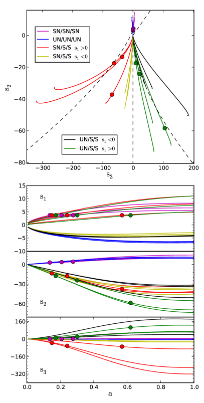
Figure 6.— Dynamical evolution of the invariants in the Zel’dovich approximation, for various initial conditions. Different colors represent various initial morphologies. Upper: Evolution trajectory in the two-dimensional invariants space $s_{3}-s_{2}$. Black dashed lines separate different categories at fixed $s_{1}$, which is also marked by solid circles on each trajectories. Lower: Time evolution of each invariant.

3.1. Dynamical evolution of invariants in the Zel’dovich Approximation

In Lagrangian dynamics, the mass element moves in the gravitational potential along the trajectory (Zel’dovich, 1970; Bernardeau et al., 2002)

$$\mathbf{x}(\mathbf{q},\tau)=\mathbf{q}+\mathbf{\Psi}(\mathbf{q},\tau),$$ (39)

from initial Lagrangian position $\mathbf{q}$. To first order, i.e. the Zel’dovich approximation (ZA) (Zel’dovich, 1970), the displacement field $\Psi(\mathbf{q},\tau)$ is given by

$$\nabla\cdot\Psi(\mathbf{q},\tau)=-D(\tau)\delta(\mathbf{q}),$$ (40)

where $D(\tau)$ the linear growth factor of density perturbation. In Eulerian space, this is equivalent to replacing the Poisson equation with (Munshi, 1994; Hui & Bertschinger, 1996; Bernardeau et al., 2002)

$$u_{i}(\mathbf{x},\tau) = -\frac{2f(\tau)}{3\Omega_{m}(\tau)\mathcal{H}(\tau)}\nabla_{i}\Phi(\mathbf{x},\tau),$$ (41)

which then closes the system together with Euler equation (33). Here, $\Omega_{m}(\tau)$ is the matter density fraction at epoch $\tau$, and $f=d\ln D/d\ln a$ is the growth rate. In this approximation, one finds that $\varpi,\varpi_{A}$ and $\varpi_{A^{2}}$ equal

$$\varpi = -\mathcal{H}(\tau)\mathcal{L}(\tau)s_{1}$$

$$\varpi_{A} = \mathcal{H}(\tau)\mathcal{L}(\tau)(s_{1}^{2}-2s_{2}),$$

$$\varpi_{A^{2}} = \mathcal{H}(\tau)\mathcal{L}(\tau)(-s_{1}^{3}+3s_{1}s_{2}-3s_{3}).$$ (42)

where we have defined $\mathcal{L}(\tau)=3\Omega_{m}(\tau)/2f(\tau)$.

Substituting Eq. (3.1) back into Eq. (3), one obtains the full dynamical equations of the invariants $s_{i}$ in the Zel’dovich approximation. They can be further simplified by defining the rescaled velocity $\bar{\mathbf{u}}=\mathbf{u}/D^{(v)}$ where $D^{(v)}(\tau)=dD/d\tau=\mathcal{H}fD$, and change the time variable $\tau$ in Eq. (33) into the linear growth rate $D$. Then, Euler equation reads (Shandarin & Zel’dovich, 1989)

$$\bar{\mathbf{u}}^{\prime}=\frac{d\bar{\mathbf{u}}}{dD}=\left(\frac{\partial}{\partial D}+\bar{\mathbf{u}}\cdot\nabla\right)\bar{\mathbf{u}}=0,$$ (43)

where the prime denotes the Lagrangian derivative $d/dD$, and we have also used differential equation of the linear growth rate Peebles (1980); Bernardeau et al. (2002)

$$\frac{d^{2}D(\tau)}{d^{2}\tau}+\mathcal{H}(\tau)\frac{dD(\tau)}{d\tau}=\frac{3}{2}\Omega_{m}(\tau)\mathcal{H}^{2}(\tau)D(\tau).$$ (44)

For the velocity gradient tensor, we similarly define the rescaled quantity $\bar{A}_{ij}=A_{ij}/D^{(v)}$, and

$$\frac{d\bar{A}_{ij}}{dD}+\bar{A}_{ik}\bar{A}_{kj}=0.$$ (45)

From the definition of various categories in Appendix A, all boundaries classifying different flow categories are invariant if the velocity is scaled with any positive number. Therefore from the definition in Eq. (2.1), we define the rescaled invariants $\bar{s}_{1},\bar{s}_{2},\bar{s}_{3}$ as

$$\bar{s}_{i}(\tau)=\frac{s_{i}(\tau)}{[D^{(v)}]^{i}},\qquad i\in\{1,2,3\}.\quad$$ (46)

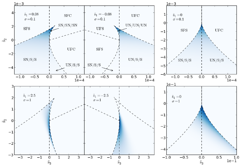
Figure 7.— Theoretical probability density of $\tilde{s}_{3}-\tilde{s}_{2}$ in the Zel’dovich approximation at $\sigma=0.1$ and $1$, for various $\tilde{s}_{1}$ ($\pm 0.08$, $0$ for $\sigma=0.1$, and $\pm 2.5$, $0$ for $\sigma=1$), assuming $\sigma=1$. The dashed lines represent boundaries among classifications, and the color scheme is the same within each plot. Notice that axes scales differently among different figures.

One can then derive a set of solvable ordinary differential equations of reduced invariants:

$$\bar{s}_{1}^{\prime}-\bar{s}_{1}^{2}+2\bar{s}_{2} = 0,$$

$$\bar{s}_{2}^{\prime}-\bar{s}_{1}\bar{s}_{2}+3\bar{s}_{3} = 0,$$

$$\bar{s}_{3}^{\prime}-\bar{s}_{1}\bar{s}_{3} = 0.$$ (47)

In Fig. (6), we plot the numerical solution of the evolution of invariants for various sets of initial conditions, where different colors indicate distinct initial flow morphologies. The upper panel illustrates the time evolution in the projected $s_{3}-s_{2}$ plane, starting from the vicinity around zero point, since $s_{i}$ roughly grows as $(D^{(v)})^{i}$ to the lowest order. The thin dashed boundaries are drawn at a certain $s_{1}$, which are marked as a solid circle on top of each trajectory. Hence even though some of the trajectories seem to visually pass through these boundary lines, it doesn’t mean the morphologies have really changed, simply because the boundaries also evolve with time. In the lower part, we also plot the time evolution of each invariant with the same color scheme.

3.2. Initial Condition and Evolution of Probability Distribution

The fact that we obtain a set of ordinary differential equations (Eq. 3.1) in the Zel’dovich approximation reflects its local assumption of the dynamical evolution, which means that the flow morphologies, and other properties of mass elements as well, decouple from the nearby environment, and are entirely determined by the initial conditions. In the Zel’dovich approximation, it is straightforward but still physically relevant to study the evolution of the distribution of the invariants $s_{i}$ away from the initial conditions.

We first notice that the velocity gradient tensor is closely related to the tensor $\xi_{ij}=\partial\Psi_{i}/\partial q_{j}(\tau)$,

$$\tilde{A}_{ij} = \frac{A_{ij}(\tau)}{d\ln D/d\tau(\tau)}=\frac{\partial\Psi_{i}(\mathbf{q},\tau)}{\partial x_{j}}=\frac{\partial\Psi_{i}(\mathbf{q},\tau)}{\partial q_{k}}(J^{-1})_{kj}.$$

For convenience, here we define another reduced quantity $\tilde{A}$, where $d\ln D/d\tau=D^{(v)}/D=\mathcal{H}f$, and $J_{ij}$ is the Jacobian matrix from Lagrangian $\mathbf{q}$ to Eulerian space $\mathbf{x}$, where $J_{ij}=\partial x_{i}/q_{j}=\ \delta_{ij}+\xi_{ij}(\tau).$ We also assume that the Jacobian is invertible, which is true before shell-crossing. Concentrating on the initial conditions, components of $\partial\Psi_{i}(\mathbf{q},\tau)/\partial q_{j}$ are small compared to unity, so $J_{ij}\sim I_{ij}$ and $\tilde{A}_{ij}\sim\xi_{ij}$. In the following, we will write all relevant quantities in this limit with superscript ^(ξ), such as $\tilde{A}^{(\xi)}_{ij}$ and $\tilde{s}^{(\xi)}_{i}$. Writing the diagonal representation of $\tilde{A}^{(\xi)}_{ij}$ as

$$\tilde{A}^{(\xi)}_{ij}=diag(\lambda_{1},\lambda_{2},\lambda_{3}),$$ (49)

with the help of the distribution function of ordered eigenvalues $\mathbf{\mathcal{P}}(\{\lambda_{i}\})$ for a Gaussian field (Doroshkevich, 1970), one could derive the distribution function of invariants $\tilde{s}^{(\xi)}_{i}$ (Bardeen et al., 1986; Pogosyan, 2009, 2010)

$$\mathbf{\mathcal{P}}\left(\left\{\tilde{s}^{(\xi)}_{i}\right\}\right) = \frac{15^{3}}{8\pi\sqrt{5}~{}\sigma^{6}}e^{-\frac{3}{2\sigma^{2}}\left[2\left(\tilde{s}^{(\xi)}_{1}\right)^{2}-5\tilde{s}^{(\xi)}_{2}\right]}$$ (50)

$$\times\ \ Real\left(\left\{\tilde{s}^{(\xi)}_{i}\right\}\right).$$

Here, the variance $\sigma$ of the density fluctuation is

$$\sigma^{2}=\frac{1}{2\pi^{2}}\int dk~{}k^{2}P(k)W^{2}(kR),$$ (51)

and $W(kR)$ is a window function with smoothing length $R$. The function $Real(\{\tilde{s}_{i}\})=\Theta(\tilde{s}_{1}^{2}-3\tilde{s}_{2})Rec(\tilde{s}_{3},\tilde{s}_{3}^{a},\tilde{s}_{3}^{b})$ defines the region in $\tilde{s}_{i}$ space with real eigenvalue solutions, where $\Theta(x)$ is Heaviside step function, and $Rec(x,x_{1},x_{2})$ is a rectangular function that equals one if $x_{1}<x<x_{2}$, and zero otherwise.

As tensor $\xi_{ij}(\tau)$ grows large enough that the effect of the Eulerian gradient becomes non-negligible, the matrix $\tilde{A}_{ij}$ becomes non-Gaussian even in the Zel’dovich approximation. With the definition Eq. (3.2), we again consider the diagonalized matrix

$$\tilde{A}_{ij}=diag(\tilde{\eta}_{1},\tilde{\eta}_{2},\tilde{\eta}_{3}).$$ (52)

In general, the eigenvector system defined by $\tilde{A}_{ij}$ and $\xi_{ij}$ will differ. However, since the addition and the inverse of a non-singular matrix does not change the eigenvectors, we have

$$\tilde{\eta}_{i}=\frac{\lambda_{i}}{1+\lambda_{i}},\qquad 1+\lambda_{i}\neq 0.$$ (53)

This allows us to estimate a Lagrangian-space (i.e. mass-weighted) PDF of the invariants of $\tilde{A}_{ij}$

$$\mathbf{\mathcal{P}}\left(\left\{\tilde{s}_{i}\right\}\right) = \mathbf{\mathcal{P}}\left(\left\{\lambda_{i}\right\}\right)\left|\frac{\partial\lambda_{i}}{\partial\tilde{\eta}_{k}}\frac{\partial\tilde{\eta}_{k}}{\partial\tilde{s}_{j}}\right|=\frac{15^{3}}{8\pi\sqrt{5}~{}\sigma^{6}~{}T^{4}}Real(\{\tilde{s}_{i}\})$$

$$\times\exp\biggl{[}\frac{-3(\tilde{s}_{1}+2\tilde{s}_{2}+3\tilde{s}_{3})^{2}}{\sigma^{2}T^{2}}+\frac{15(3\tilde{s}_{3}+\tilde{s}_{2})}{2\sigma^{2}T}\biggr{]},$$

where we have defined the notation

$$T=1+\sum_{i}\tilde{s}_{i}=1+\tilde{s}_{1}+\tilde{s}_{2}+\tilde{s}_{3}.$$ (55)

$Real(\tilde{s}_{i})$ is the same function defined previously.

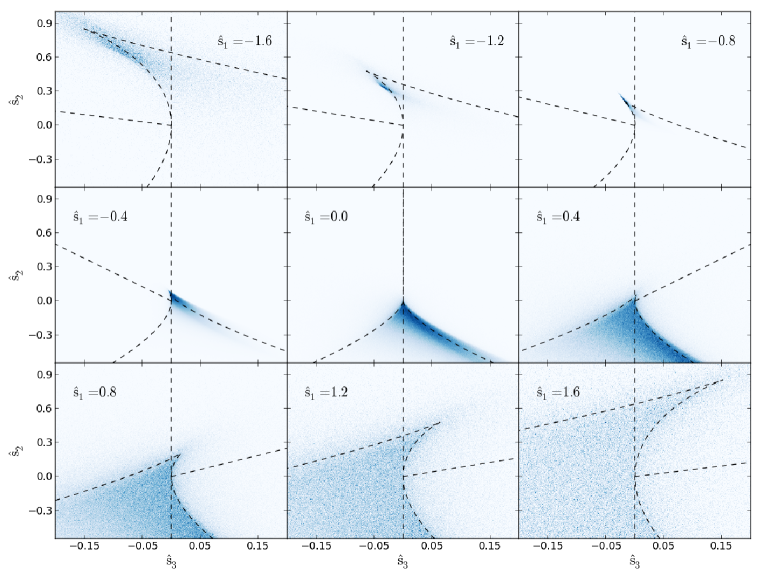
Figure 8.— Two-dimensional probability of $\hat{s}_{3}$ and $\hat{s}_{2}$ for nine different bins of $\hat{s}_{1}$, measured from simulations at $z=0$. Note that the hat quantities $\hat{s}_{i}$ denote the rescaling of the tensor $A_{ij}$ Eq. (56) so that invariants are confined within given rectangular region. From left to right, $\hat{s}_{1}$ goes from $-1.6,-1.2,-0.8$ in the first row, to $-0.4,0,0.4$ in the middle, and then to $0.8,1.2,1.6$ in the bottom row. At larger $|\hat{s}_{1}|$, mass elements are more likely to spread into vortical regions, although part of the spreading is due to our finite bin size of $\hat{s}_{1}$.

In Fig. (7), we show the two-dimensional probability distribution of $\tilde{s}_{3}-\tilde{s}_{2}$ at two different $\tilde{s}_{1}$’s. For the dispersion, we use $\sigma=0.1$ to represent an initial epoch in the first row, and $\sigma=1$ for a later time in the second. Similar to previous figures, the dashed lines illustrate the boundaries between classifications. Since initial conditions with the same $\tilde{s}_{1}(\tau_{init})$ but different $\tilde{s}_{2}(\tau_{init})$ and $\tilde{s}_{3}(\tau_{init})$ do not necessarily evolve to the same $\tilde{s}_{1}(\tau_{final})$, a comparison of the two-dimensional probability distribution at given $\tilde{s}_{1}$ between two epochs is by no means rigorous as they do not consist of the same set of samples. Therefore, the values of $\tilde{s}_{1}$ for plotting the figure are chosen more or less arbitrarily. Nevertheless, one still notices that the asymmetry increases with $\sigma$. This statement remains valid and is even more evident for $\tilde{s}_{1}=0$ since initially $\tilde{s}_{2,3}$ are symmetrically distributed. However, the skewed distribution in the lower panels does not necessarily mean the probability of a Lagrangian fluid element belonging to a particular morphology changes with time significantly in the ZA, because $\tilde{s}_{1}$ as well as the morphology boundaries evolve together and the sample points contributing to the last panel at $\tilde{s}_{1}=0$ come from various initial $\tilde{s}_{1}(\tau_{init})$.

3.3. Nonlinear Evolution beyond Zel’dovich Approximation

Even without the shell-crossing, the gravitational nonlinearity of the system (Eq. 34-36) already makes the analytical study of the evolution of velocity gradient invariants very complicated. One possibility is to investigate the Lagrangian evolution of all relevant quantities at least numerically, similar to Eq. (3.1) in ZA, but including density $\delta$, velocity gradient $A_{ij}$ as well as the tidal tensor $\varepsilon_{ij}=\varpi_{ij}-\varpi\delta_{ij}/3$, which however, does not exist in Newtonian cosmology due to the nonlocality of the theory. In the following, we will only concentrate on the numerical measurement from the simulation.

In Fig. (8), we show the two-dimensional probability distribution of the invariants from the $N$-body simulations ‘$Sing100$’. Instead of measuring the invariants themselves, we normalize the velocity gradient tensor

$$\hat{A}_{ij}=\frac{A_{ij}}{\sqrt{A_{mn}A_{mn}}}$$ (56)

first, given that any rescaling of $A_{ij}$ with a positive constant would not change the boundaries between kinematic classes. After this normalization, the invariants are confined within the cubic region $\hat{s}_{1}\in[-\sqrt{3},\sqrt{3}]$, $\hat{s}_{2}\in[-1/2,1]$ and $\hat{s}_{3}\in[-\sqrt{3}/9,\sqrt{3}/9]$. From top to bottom, left to right, we plot the distribution at $\hat{s}_{1}=(-1.6,-1.2,-0.8,-0.4,0,0.4,0.8,1.2,1.6)$. Before further preceding, one should realize that a direct comparison between Fig. (7) and (8) could be misleading, because here we are measuring the volume-weighted probability distribution in Eulerian space, whereas Fig. (7) is mass-weighted. A consistent comparison of various theoretical models as well as simulations in both Eulerian and Lagrangian space is indeed desired, but will not be the main topic of this paper.

Note that the whole dataset is divided into nine thick $\hat{s}_{1}$ bins, while the dashed boundaries in each panel correspond to the median value of $\hat{s}_{1}$ in each bin. In panels with medium $\hat{s}_{1}$ where the shape of the distribution is sharp and clear, one would expect most of the offset is due to this finite bin size effect. This includes at least from the third to the sixth panel in the figure, because the sample points at these $\hat{s}_{1}$ bins are much more than the other. The fraction of data in all nine panels are $\{0.003,0.009,0.38,0.31,0.15,0.06,0.041,0.029,0.018\}$ respectively. For the first two panels at $\hat{s}_{1}=-1.6$ and $-1.2$, however, theoretical argument may suggest the same since it corresponds to the outflowing void region where gravitational nonlinearity is less significant. In the bottom panels with large positive $\hat{s}_{1}$, in which regions the fluid elements collapse fast enough, the PDFs are much flatter, and there is much spreading, especially in the last two panels. This could be attributed to both the nonlinear evolution as well as the effect of shell-crossing.

Figure 9.— PDF of the cosine of the angle between velocity and vorticity as measured in all $64$ realizations of MIP simulation. The alignment is strongest for categories ‘$\mathcal{SFS}$’ and ‘$\mathcal{UFC}$’, which trace filamentary structure.

4. Shell-crossing and Emergence of Vorticity

In the multi-streaming regime, vorticity is often generated. Since velocity and density perturbations are strongly coupled, it is reasonable to expect that rotational degrees of freedom correlate with large-scale structures, as in the potential flow. Indeed, from the N-body simulation, we do observe this associations not only via the distinct spatial distribution of various vortical flows, but also the alignment between the vorticity and the cosmic web. The theory, as will be seen later in this section, is complicated and highly non-trivial quantitatively. One obstacle is to incorporate the shell-crossing in a closed dynamical fluid system. To do so, we start from the fundamental Vlasov-Poisson system, and then derive evolution equations of invariants including phase space information of multi-streaming. However, instead of solving the dynamical system, we alternatively try to propose a statistical description which relates to the internal structure of the invariants space.

4.1. The Spatial and Orientation Distribution of Vorticity

Figure 10.— The alignment between the vorticity and the eigenvectors $e_{i}$ of the density Hessian matrix for various rotational categories. The density field is smoothed with a Gaussian filter with smoothing length $R=1{\rm Mpc}/h$ and $0.5{\rm Mpc}/h$, as shown in solid and dashed lines, respectively. Similar to Fig. (9), the alignment is strongest for categories ‘$\mathcal{SFS}$’ and ‘$\mathcal{UFC}$’, which trace filamentary structure.

The distinct spatial distributions revealed in both potential and rotational flows suggest that the emergence of vorticity could in principle relate to the cosmic web. Unlike in irrotational flow, the spatial distribution of all categories shown in Fig. (3) are visually correlated with filaments, walls, and knots, where shell-crossing takes place. This is especially clear for the categories ‘$\mathcal{SFS}$’ and ‘$\mathcal{UFC}$’ with smaller $n_{ct}$, i.e. the last row in the figure, when almost all visible filaments have been painted by those labels. Together with flow trajectories illustrated in Fig. (1), the spatial distribution of some categories also seems to be consistent with physical intuition. For example, within knots, the spatial contraction and the energy transfer from direct infall to orbiting leads to the inward winding and compression along the radial direction, i.e. the ‘$\mathcal{SFC}$’ category. And the type of vorticity generated along filaments funneling matter to knots should involve inward spiraling and stretching. However, one also notices that this agreement is not as large as one would naively expected. On the one hand, this reveals the complexity of the problem; on the other hand, it might suggest a statistical/stochastic view of the vorticity generation.

This interpretation can be further verified by examining the alignment between the direction of the vorticity, the velocity and the cosmic web structure. In Fig. (9), we first present the distribution of the angle between vorticity and velocity for various categories. Two of them, which interestingly mainly trace the filamentary structures, show the most significant correlation signal between the direction of these two vectors, but in an opposite way. In ‘$\mathcal{SFS}$,’ the velocity tends to be aligned with vorticity, and in type ‘$\mathcal{UFC}$,’ the velocity tends to be perpendicular. In general, although not as obviously as in previous examples, mass elements seem to flow along the vorticity direction if it is stretching, and tends to flow perpendicularly when compressing along the direction of vorticity.

Fig. 10 shows the alignment of the vorticity with cosmic-web structure. We display the angle distribution between the vorticity and eigenvectors of the density Hessian matrix $\nabla_{i}\nabla_{j}\rho$, for different vortical categories. Here $e_{i}$ denotes the $i$th eigenvector, with eigenvalue $\lambda_{i}$, where $\lambda_{i}$ are sorted according to the absolute value, $|\lambda_{1}|\leq|\lambda_{2}|\leq|\lambda_{3}|$. Therefore, $e_{1}$ corresponds to the direction with slowest changing rate of density distribution, and $e_{3}$ the fastest. In filaments, $e_{1}$ is aligned with the filament’s axis. We smoothed the density field with a Gaussian filter at smoothing length $R=0.5{\rm Mpc}/h$ and $1{\rm Mpc}/h$. Similar to the situation in velocity-vorticity alignment, the correlation is strongest for categories ‘$\mathcal{SFS}$’ and ‘$\mathcal{UFC}$’, which trace the filaments. Particularly, type ‘$\mathcal{SFS}$’ is more aligned with the direction of smallest eigenvalues $|\lambda_{1}|$. On the other hand, one could also see the distinctive alignment of ‘$\mathcal{UFC}$’, where the vorticity is perpendicular to $|\lambda_{1}|$, and parallel with $|\lambda_{2}|$ or $|\lambda_{3}|$. We also notice the smoothing variations that has been encountered by Codis et al. (2012) and Aragon-Calvo (2013).

Fig. (9) together with Fig. (10) reinforce our previous physical interpretation. For instance, they show that the vorticity direction of ‘$\mathcal{SFS}$’ type aligns with both velocity as well as the filament directions. Given its schematic flow trajectory from Fig. (1), this is consistent with the physical picture of the accretion along filament with additional rotation around the main path (Pichon et al., 2011; Codis et al., 2012; Laigle et al., 2013), which is expected to be generated during the formation of filamentary structure (Zel’dovich, 1970; Bond et al., 1996; Pichon et al., 2011). For category ‘$\mathcal{UFC}$’, since the vorticity direction is perpendicular to both filament and velocity, the major component of the velocity is still along the filament. This suggests that vorticity of this type is related to halo spin formed by major mergers along the filaments (Codis et al., 2012). Therefore as demonstrated above, shell-crossing and generation of vorticity are physically rich processes. In the invariants space, this means certain types of trajectories exist transitioning from potential flow to a particular rotational flow region, which as will be seen later is the main focus of this section.

4.2. Emergence of Vorticity: Dynamical View

Before discussing our statistical view of vorticity generation, let us go back to examine the dynamical system first. To proceed, one has to restore the extra source contribution of the velocity dispersion in the Euler equation (33), because the term $\varpi_{ij}$ in Eq. (36) is symmetric, therefore initial irrotational flow will not be able to generate vorticity. The standard approach is to start from the more fundamental Vlasov equation of one-particle phase-space density $f(\mathbf{x},\mathbf{p},\tau)$ (Peebles, 1980; Bernardeau et al., 2002),

$$\frac{\partial f}{\partial\tau}+\frac{\mathbf{p}}{am}\cdot\frac{\partial f}{\partial\mathbf{x}}-am\nabla\Phi\cdot\frac{\partial f}{\partial\mathbf{p}}=0,$$ (57)

and then take moments of the velocity, given the fluid quantities defined as

$$\rho = \int d^{3}\mathbf{p}~{}f(\mathbf{x},\mathbf{p},\tau),\quad u_{i}=\int d^{3}\mathbf{p}~{}f(\mathbf{x},\mathbf{p},\tau)~{}\frac{p_{i}}{am},$$

$$\varsigma_{ij} = \int d^{3}\mathbf{p}~{}f(\mathbf{x},\mathbf{p},\tau)~{}\left(\frac{p_{i}}{am}-u_{i}\right)\left(\frac{p_{j}}{am}-u_{j}\right),$$ (58)

Here $\mathbf{x}$ and $\mathbf{p}=am\mathbf{u}$ are the comoving positions and momenta of particles, with $m$ the mass of particle and $\mathbf{u}$ the peculiar velocity. And $\varsigma_{ij}$ is the velocity dispersion, and has been ignored in the previous dust model. Eventually one recovers the Euler equation with an extra term,

$$\frac{\partial\mathbf{u}}{\partial\tau}+\mathcal{H}(\tau)\mathbf{u}(\mathbf{x},\tau)+\mathbf{u}(\mathbf{x},\tau)\cdot\nabla\mathbf{u}(\mathbf{x},\tau)=\quad\qquad$$

$$-\nabla\Phi(\mathbf{x},\tau)-\frac{1}{\rho}\nabla_{j}(\rho\varsigma_{ij}).\qquad$$ (59)

The gradient tensor $A_{ij}$ reads as

$$\frac{dA_{ij}}{d\tau}+\mathcal{H}(\tau)A_{ij}+A_{ik}A_{kj}=\varpi_{ij}+\zeta_{ij},$$ (60)

and here we define the ‘dispersion tensor’ $\zeta_{ij}$ as

$$\zeta_{ij}=-\nabla_{j}\left[\frac{1}{\rho}\nabla_{k}\left(\rho\varsigma_{ik}\right)\right].$$ (61)

Replacing $\varpi_{ij}$ and its derivatives with $\varpi_{ij}+\zeta_{ij}$ in Eq. (3), one obtains dynamical equations of invariants with extra source terms,

$$\frac{d}{d\tau}s_{1}+\mathcal{H}(\tau)s_{1}-s_{1}^{2}+2s_{2} = -\varpi-\zeta\$$

$$\frac{d}{d\tau}s_{2}+2\mathcal{H}(\tau)s_{2}-s_{1}s_{2}+3s_{3} = -s_{1}(\varpi+\zeta)-\varpi_{A}-\zeta_{A}$$

$$\frac{d}{d\tau}s_{3}+3\mathcal{H}(\tau)s_{3}-s_{1}s_{3} = -s_{2}(\varpi+\zeta)-s_{1}(\varpi_{A}$$ (62)

$$+\zeta_{A})-\varpi_{A^{2}}-\zeta_{A^{2}}.\quad$$

However, the system has to be closed, i.e. the infinite hierarchy series needs to be truncated (Pueblas & Scoccimarro, 2009). A handful of suggestions have been proposed (Pueblas & Scoccimarro, 2009; Dominguez, 2000; Buchert & Domínguez, 2005). In general, one desires to know the full phase space information from Eq. (57).

4.3. Emergence of Vorticity: Statistical View

Instead of explicitly solving the dynamical system discussed previously, as will be seen later, it is also possible to establish a statistical description for generation of vorticity in the invariants space. In the multi-streaming region, one defines the bulk velocity which projected from the phase space as the density-weighted average among all streams

$$\mathbf{u}(\mathbf{x})=\frac{1}{\rho(\mathbf{x})}\sum_{s}\rho(\mathbf{q}_{s})\mathbf{u}(\mathbf{q}_{s}),$$ (63)

where $\rho(\mathbf{q}_{s})$ and $\mathbf{u}(\mathbf{q}_{s})$ are density and velocity of each stream, and $\rho(\mathbf{x})=\sum_{s}\rho(\mathbf{q}_{s})$ is the Euerlian density. Then by taking the gradient of Eq. (63), one notices two separate contributions to the averaged gradient tensor $A_{ij}$: first is the density average of $A^{s}_{ij}$ among all streams

$$\frac{1}{\rho(\mathbf{x})}\sum_{s}\left[\rho(\mathbf{q}_{s})A^{s}_{ij}(\mathbf{q}_{s})\right],$$ (64)

and the other is the coupling between the density gradient and velocity arising purely due to the projection of a multi-valued field from the phase space (Pichon & Bernardeau, 1999; Hahn et al., 2014),

$$\frac{1}{\rho(\mathbf{x})}\biggl{[}\sum_{s}u_{i}(\mathbf{q}_{s})\frac{\partial}{\partial x_{j}}\rho(\mathbf{q}_{s})-u_{i}(\mathbf{x})\frac{\partial}{\partial x_{j}}\rho(\mathbf{x})\biggr{]}.\qquad$$ (65)

In the cold-dark-matter scenario, matter is assumed to reside on a three dimensional thin sheet in the six dimensional phase space. The generalized Kelvin’s circulation theorem then ensures that the average vorticity will remain zero within any circle in phase space (Lynden-Bell, 1967), and it is also zero for all closed loops in three-dimensional position space which are non-intersecting when projected from six dimensions. However, in the multi-streaming region after shell-crossing, a simple circle in phase space could be projected down as interacting ‘$8$’-like loops, with nonzero vorticity for each of them in three-dimensional position space. Yet, depending on the scale of interest, at any epoch, one is free to choose loops have not been deformed large enough to generate any net effect except near the vicinity of singular points, which might become non-negligible in the deeply nonlinear regime, for example in viralized halos.

For simplicity, we would like to assume the velocity of each stream is still potential after shell-crossing, so the first contribution (Eq. 64) of $A_{ij}$ is symmetric. Then, rotation arises from the coupling between density gradient and the velocity of streams (Eq. 65). Since various morphological structures are distinct in the density gradient as well as their coupling with the velocity field, this contribution depends on the environment. This could be responsible for the different spatial and orientation distribution of various vortical categories.

4.3.1 Shell-crossing in the Invariants Space

Given the expression of $A_{ij}$ in Eq. (64) and (65), it is possible to set up a statistical description of the vorticity emergence in the invariants space. At arbitrary Eulerian position $\mathbf{x}$, we assume there are many streams, labeled from $1$ to $\alpha$, flowing potentially, and we denote the invariants as

$${}^{1\cdots\alpha}s^{(s)}_{i}=\{^{1}s^{(s)}_{i},~{}^{2}s^{(s)}_{i},~{}\cdots~{}^{\alpha}s^{(s)}_{i}\},~{}i=(1,2,3)\qquad$$ (66)

where ${}^{m}s^{(s)}_{i}$ are potential invariants for $m$th stream, and they have the probability distribution

$$\mathbf{\mathcal{P}}\left({}^{1\cdots\alpha}s^{(s)}_{i}\right).$$ (67)

As seen in previous sections, this distribution characterizes the morphological information of the cosmic web. After a short yet finite amount of time $\Delta\tau$, the winding of the dark matter sheet in the phase space becomes large enough to form a multi-streaming region. These $\alpha$ streams encounter and couple with each other to generate final invariants $s_{i}$ through Eqs. (64) and (65), with distribution functions $\mathbf{\mathcal{P}}(s_{i})$. This shell-crossing process can then be described by the conditional probability distribution of final $s_{i}$’s given initial invariants ${}^{1}s^{(s)}_{i}\cdots~{}^{\alpha}s^{(s)}_{i}$

$$\mathbf{\mathcal{P}}(s_{i}|~{}^{1\cdots\alpha}s^{(s)}_{i}).$$ (68)

From Eq. (65), these distributions also encode information about cosmic-web morphologies, since velocity and density gradients couple differently depending on the environment. Here we explicitly write down the time lapse $\Delta\tau$ to simplify the description, since in reality, multi-value regions emerge gradually, from three-flow regions to more complicated cases. In this situation, if shell crossings occur more than $m$ times during $\Delta\tau$, what happens is essentially a random walk in invariants space, where the final distribution $\mathbf{\mathcal{P}}_{\Delta\tau}(s_{i}|~{}^{1\cdots\alpha}s^{(s)}_{i})$ is a series multiplication of separate probability functions

$$\mathbf{\mathcal{P}}_{\Delta\tau}(s_{i}|~{}^{1\cdots\alpha}s^{(s)}_{i})=\prod_{m}\mathbf{\mathcal{P}}_{\tau_{m}}(^{1\cdots\alpha}s_{i}(m)|~{}^{1\cdots\alpha}s_{i}(m-1)).$$

Here we assume at each step, only a subset $\tau_{m}(1\cdots\alpha)$ was involved in the process.

4.3.2 Boundary Crossing and the Internal Structure of Invariants Space

To further investigate the validity of this description, we explore the probability distribution $\mathbf{\mathcal{P}}(s_{i}|^{1\cdots\alpha}s^{(s)}_{i})$ numerically, and show the result in Table (1). At an arbitrary location where shell-crossing occurs, we assume that a random number of streams overlap. From Eq. (64) and Eq.  (65), both the symmetric and anti-symmetric contributions are environmentally dependent, so we first generate samples of $A^{s}_{ij}$ for various kinematical categories from Zel’dovich approximation, and identify these irrotational kinematical types as morphology structures. That is, we consider ‘$\mathcal{SN/SN/SN}$’ as halo, ‘$\mathcal{SN/S/S}$’ as filament and ‘$\mathcal{UN/S/S}$’ as wall structures. Then based on their morphological classes, we generate velocity as well as the density gradient for all flow elements, which roughly resemble the physical process near each morphological structure. For example, both the velocity vectors and density gradients are sampled spherically for halos. The velocities are assumed to flow close to a line for filaments, and the density gradients around the radial direction of a cylinder. And near the wall, both velocities and density gradients are chosen close to a given direction. With $u_{i}$, $\nabla_{i}\rho$, and $A^{s}_{ij}$ for each stream, we are then able to construct the full velocity gradient tensor $A_{ij}$ via Eqs. (64) and (65).

Table 1 Kinematic morphologies generated by the toy model of stream-crossing

	$\mathcal{SN/SN/SN}$ (halo)	$\mathcal{SN/S/S}$ (filament)	$\mathcal{UN/S/S}$ (wall )	$\mathcal{UN/UN/UN}$ (void )	$total~{}(after)$
$\mathcal{SN/SN/SN}$	$0.3~{}(10.1)$	$0.5~{}(1.6)$	$0.3~{}(0.5)$	$-$	$1.1$
$\mathcal{SN/S/S}$	$1.1~{}(34.3)$	$10.5~{}(37.0)$	$11.3~{}(22.5)$	$-$	$22.9$
$\mathcal{UN/S/S}$	$0.2~{}(6.0)$	$4.3~{}(15.1)$	$25.8~{}(51.3)$	$-$	$30.3$
$\mathcal{UN/UN/UN}$	$0.0~{}(0.0)$	$0.1~{}(0.2)$	$3.6~{}(7.1)$	$18.2~{}(100)$	$21.8$
$\mathcal{SFS}$	$0.4~{}(13.2)$	$5.3~{}(18.5)$	$2.6~{}(5.2)$	$-$	$8.3$
$\mathcal{UFS}$	$0.0~{}(0.4)$	$0.6~{}(2.1)$	$2.5~{}(5.0)$	$-$	$3.1$
$\mathcal{SFC}$	$0.8~{}(26.5)$	$2.3~{}(8.0)$	$0.6~{}(1.1)$	$-$	$3.7$
$\mathcal{UFC}$	$0.3~{}(9.5)$	$4.9~{}(17.4)$	$3.6~{}(7.1)$	$-$	$8.8$
$total~{}(before)$	$3.2~{}(100)$	$28.4~{}(100)$	$50.2~{}(100)$	$18.2~{}(100)$	$100$

Each column shows the percentage of flow morphologies generated from particular type displayed at the top, numbers in parentheses give the normalized fraction within every column, i.e. the probability of generating other categories from that morphology. The last row/column is the marginal sum of each column/row. Therefore, the last row gives the total fraction of each morphologies before the crossing, and the last column gives total percentage after crossing. To compare with the spatial distributions in Fig. (3), the pre-crossing fractions, i.e. the last row, are volume-weighted in Eulerian space at redshift $z=2$. All numbers are displayed in percentage (%), and have been rounded for display purpose. The dashes in the column of void means our model does not assume any stream-crossing in void region, and therefore they are set to be zero.

We also list the fractions of all kinematical types generated by our numerical shell-crossing model in Table (1). The total number of samples we generated is the roughly the order of $256^{3}$. Each column corresponds to a particular morphological structure we started from, which from left to right are halo ‘$\mathcal{SN/SN/SN}$’, filament ‘$\mathcal{SN/S/S}$’, wall ‘$\mathcal{UN/S/S}$’ and void ‘$\mathcal{UN/UN/UN}$’. In our probably over-simplified toy model, stream-crossing happens for streams with the same kinematical class. After that, however, all categories can be generated, including both potential and vortical classes, as shown in different rows. In the table, we list in each column the percentage of flow morphologies generated from the particular type displayed at the top, numbers in parentheses give the normalized probability within every column. The last row gives the total volume weighted fraction of each morphologies before the crossing, and the last column gives total percentage after the crossing.

From the table, physically implausible situations, like voids generated in highly multi-streaming filaments and halos, are produced only in very tiny amount. Although a substantial fraction of potential flows are produced, we are more interested in the vortical ones. From the table, there are higher probabilities to generate vorticity with class ‘$\mathcal{SFC}$’ around halos ($26.5\%$ compared with $13.2\%$ of ‘$\mathcal{SFS}$’ and $9.5\%$ of ‘$\mathcal{UFC}$’); type ‘$\mathcal{SFS}$’ ($18.5\%$) as well as ‘$\mathcal{UFC}$’ ($17.4\%$) near filaments; and a similar fraction of almost all vortical types around walls. Given the simplicity of our model, the exact value in Table (1) should not be taken too seriously. However, from the fifth row of the table, among $8.3\%$ of vortical category ‘$\mathcal{SFS}$’ being generated from stream crossing, more than sixty percents of them are formed near filaments ‘$\mathcal{SN/S/S}$’. And this is also true for category ‘$\mathcal{UFC}$’ ($4.9\%$ compares with $8.8\%$ in total). From Fig. (3), this is exactly what one found from the filamentary spatial distribution of these two categories. For type ‘$\mathcal{SFC}$’, however, due to small fraction of type ‘$\mathcal{SN/SN/SN}$’ initially, the dominant contribution comes from filaments. This might also be physically plausible since the spatial distribution of this type tends to extend a little from central halos to the filamentary structures. Finally, both our model and Fig. (3) suggest type ‘$\mathcal{UFC}$’ is more likely to be generated in walls ($2.5\%$ compares with $3.1\%$ in total).

Even without any detailed information about the conditional distribution of the shell-crossing $\mathbf{\mathcal{P}}(s_{i}|^{1\dots\alpha}s^{(s)}_{i})$, it is not hard to understand the result, since from Fig. (1), one discovers that the region of irrotational flow that follows the filament structures (‘$\mathcal{SN/S/S}$’) is just adjacent to the ‘$\mathcal{SFS}$’ vortical region in invariants space, which also is associated with filaments. Similarly, the triangle-like region of halos ‘$\mathcal{SN/SN/SN}$’ resides just inside the ‘$\mathcal{SFC}$’ regime. Physically, this is also consistent with the formation of cosmic web structures. Consider mass elements flowing around filaments potentially. In the canonical form of the tensor $A_{ij}$, there are three real eigenvalues $\lambda_{i}$. At some point, shell-crossing occurs, and from Zel’dovich’s structure-formation theory, the filaments are formed from the second collapse, after walls. The trajectory in position space will produce a spiral in the plane perpendicular to the filament. In the idealized case where $\lambda_{1}\sim\lambda_{2}<0$ for any of two eigenvalues initially, and only small amount $\epsilon$ has been changed to the real part of $\lambda_{1}$, one obtains the canonical form

$$\mathbf{A}=\left(\begin{array}[]{ccc}\lambda_{1}+\epsilon&-b&\\ b&\lambda_{1}+\epsilon&\\ &&\lambda_{3}\\ \end{array}\right).$$ (73)

From Eq. (2.2.2), in this case, $s_{2}$ will be enlarged and $s_{3}$ will be smaller, giving a shift in the upper-left direction in the invariants space. So, just around filaments, category ‘$\mathcal{SFS}$’ will be generated, and the spatial association with the large-scale structure is preserved after shell-crossing. Furthermore, this physical picture also suggests that the vorticity direction is aligned with filaments, consistent with our measurement in simulation for this category. The situation around halos is even simpler, since from Fig. (1), category ‘$\mathcal{SN/SN/SN}$’ is almost entirely surrounded by the ‘$\mathcal{SFC}$’ type in the invariants space. And therefore it gives much higher probability to generate this type of rotational flow around halos.

5. Conclusion and Discussions

In this paper, we concentrated on the velocity gradient tensor $A_{ij}$ and its rotational invariants defined as coefficients of the characteristic equation of $A_{ij}$. They enable one to classify all possible flow patterns including both potential and rotational flows. For irrotational flow, our invariants-based categorization is equivalent to the cosmic web finder ‘V-web’ (Hoffman et al., 2012) with the threshold eigenvalue $\lambda_{th}=0$. The PDF of density and fractional anisotropy of various flows are consistent with their morphology types, although the visual impression of the web structure might not be as accurate as other techniques (Pogosyan et al., 2009; Aragon-Calvo et al., 2010; Sousbie, 2011a, b; Bond et al., 2010; Forero-Romero et al., 2009; Hahn et al., 2007a; Sousbie et al., 2009; Stoica et al., 2005; Hoffman et al., 2012). To improve it, one could introduce a non-zero fine-tuned threshold $\lambda_{th}$ as done in the ‘V-web’ finder. In our method, this can be achieved by a simple invariants transformation (Eq. 2.2.1). However, from the fractional anisotropy distribution, the physical interpretation might become difficult. Since all invariants are one-to-one mapped to eigenvalues, they could also be applied to other dynamical classification methods, e.g. invariants defined for deformation tensor or the Hessian matrix of gravitational potential (Hahn et al., 2007a; Forero-Romero et al., 2009).

As a region develops vorticity, the invariants change continuously, which is a clear benefit of working with these invariants. By combining an ensemble of $N$-body simulations with the same large-scale modes, we show that various rotational flows also trace the cosmic web structure differently. This reveals the dynamical nature of these variables and provides an alternative view on the emergence of vorticity. Therefore, an understanding of their dynamical evolution would be valuable. We first stepped back and concentrated on the irrotational flow, which is important on its own as the indicator of cosmic web, and started from the simplest Zel’dovich approximation, where both accurate solution of time evolution and the analytical formula of PDF are available. We also wrote down a set of dynamical equations for the invariants from the Euler equation. However, further investigation is difficult due to the gravitational nonlinearity. One possibility is to study the Lagrangian evolution of all relevant quantities, including the density $\delta$, velocity gradient $A_{ij}$, and the tidal tensor $\epsilon_{ij}=\varpi_{ij}-\varpi\delta_{ij}/3$. Due to the non-locality of Newtonian cosmology, the evolution equation of $\epsilon_{ij}$ is missing, and will only be feasible under certain approximation. We will follow this approach in a separate paper (Wang et al., in prep.).

Given the complications of dynamical modeling of the nonlinear gravitational evolution as well as the shell-crossing, the key insight came after realizing the stochastic nature of the multi-streaming. The distinctive spatial distribution of different rotational flow morphologies is very likely to be a consequence of some diffusion process in the invariants space. Indeed, the internal structure of the invariants space (Fig. 1) shows the adjacency between the potential morphology ‘$\mathcal{SN/SN/SN}$’ and rotational type ‘$\mathcal{SFC}$’ who both spatially follow halos, and the contiguity between type ‘$\mathcal{SN/S/S}$’ and ‘$\mathcal{SFS}$’ which all appear around filaments. Without any sophisticated model, we numerically investigated the PDF of invariants generated from a toy model of stream-crossing. The result in Table. (1) qualitatively supports our conjecture.

However, many details of this stochastic process are still missing. For example, it is unclear whether a simple diffusion would be able to explain the physics associated with halo formation. Unlike the vorticity, the angular momenta of halos can be formed from laminar flow by the misalignment between the shear and inertia of given region which encloses the material of a protogalaxy, i.e. from the tidal torque theory (Hoyle, 1949; Peebles, 1969; Doroshkevich, 1970; White, 1984; Wesson, 1985). Compared with the fast growth $\sim D^{6.5/2}$ (Pueblas & Scoccimarro, 2009) of vorticity after its emergence, the halo spin grows slower since the very early stages of structure formation. However, as suggested by Libeskind et al. (2013a), the strong alignment between the direction of vorticity and halo angular momentum suggests another phase of the coevolution between them after the tidal torque becomes ineffective after turn-around when the lever arm is dramatically reduced.

This coevolution phase seems to be reasonable since as in our findings of two different alignments between vorticity and filaments (category ‘$\mathcal{SFS}$’ and ‘$\mathcal{UFC}$’ respectively), recent studies also suggest two states of preferential orientation between halo spins and filaments (Hahn et al., 2007a; Sousbie et al., 2009; Zhang et al., 2009; Codis et al., 2012; Aragon-Calvo, 2013). Moreover, it has been confirmed that this orientation is mass-dependent (Codis et al., 2012), i.e. low-mass halos tend to be aligned with filaments, and high-mass halos have spin perpendicular to the filaments (Aragon-Calvo et al., 2007; Hahn et al., 2007b; Paz et al., 2008; Codis et al., 2012). Codis et al. (2012) proposed an interpretation that more massive halos acquire their spins that perpendicular to the filaments via merger process along filament. If this is the case, the trajectories of a mass element in the invariants space might be much more complicated. Further investigations of how such process would manifest itself in the invariants space would be interesting.

Appendix Appendix A List of Classification

Most results in this appendix are originally from Chong et al. (1990). We quote the results here for the purpose of completeness. Considering the solution to the characteristic equation

$$\det[\mathbf{A}-\lambda\mathbf{I}]=\lambda^{3}+s_{1}\lambda^{2}+s_{2}\lambda+s_{3}=0,$$ (A1)

one can look at the coefficient space $\{s_{1},s_{2},s_{3}\}$. The surface $S_{1}$ that divides the real and complex solutions is given by

$$27s_{3}^{2}+(4s_{1}^{3}-18s_{1}s_{2})s_{3}+(4s_{2}^{3}-s_{1}^{2}s_{2}^{2})=0$$ (A2)

Denoting the solution of the above equation as $s_{3a}$ and $s_{3b}$, assuming $s_{3a}\leq s_{3b}$, regions with real eigenvalues at fixed $s_{1}$ correspond to

$$s_{2}\leq s_{1}^{2}/3,\qquad s_{3a}\leq s_{3}\leq s_{3b}.$$ (A3)

When either equal sign of the second inequality holds, two of eigenvalues will be equal. And if the first equality also holds, one gets three real and equal eigenvalues.

For the purpose of cosmology, we are particularly interested in the following potential flow categories:

$$Stable~{}Nodes~{}(\mathcal{SN/SN/SN}): ~{}~{}s_{1}>0,\qquad 0<s_{2}<s_{1}^{2}/3,\qquad\max(s_{3a},0)<s_{3}<s_{3b},$$

$$Stable~{}Node/Saddle~{}(\mathcal{SN/S/S}): ~{}~{}s_{1}\geq 0,\qquad s_{2}<s_{1}^{2}/4,\qquad s_{3a}<s_{3}<0,$$

$$or ~{}~{}s_{1}<0,\qquad s_{2}<0,\qquad s_{3a}<s_{3}<0.$$

$$Unstable~{}Node/Saddle~{}(\mathcal{UN/S/S}): ~{}~{}s_{1}\leq 0,\qquad s_{2}<s_{1}^{2}/4,\qquad 0<s_{3}<s_{3b},$$

$$or ~{}~{}s_{1}>0,\qquad s_{2}<0,\qquad 0<s_{3}<s_{3b}.$$

$$Unstable~{}Nodes~{}(\mathcal{UN/UN/UN}): ~{}~{}s_{1}<0,\qquad 0<s_{2}<s_{1}^{2}/3,\qquad s_{3a}<s_{3}<\min(s_{3b},0),$$ (A4)

where we list in the order of halo, filament, wall and void. And for vortical flow, we have

$$Stable~{}Focal~{}Stretching~{}(\mathcal{SFS}): ~{}~{}s_{1}\geq 0,\qquad s_{2}>s_{1}^{2}/4,\qquad s_{3}<0,$$

$$or ~{}~{}s_{1}\geq 0,\qquad s_{2}<s_{1}^{2}/4,\qquad s_{3}<s_{sa},$$

$$or ~{}~{}s_{1}<0,\qquad s_{2}>0,\qquad s_{3}<s_{1}s_{2},$$

$$or ~{}~{}s_{1}<0,\qquad s_{2}<0,\qquad s_{3}<s_{sa},$$

$$Stable~{}Focal~{}Compressing~{}(\mathcal{SFC}): ~{}~{}s_{1}>0,\qquad s_{2}>s_{1}^{2}/3,\qquad 0<s_{3}<s_{1}s_{2},$$

$$or ~{}~{}s_{1}>0,\qquad s_{1}^{2}/4<s_{2}<s_{1}^{2}/3,\qquad 0<s_{3}<s_{sa},$$

$$or ~{}~{}s_{1}>0,\qquad 0<s_{2}\leq s_{1}^{2}/3,\qquad s_{3b}<s_{3}<s_{1}s_{2}$$

$$Unstable~{}Focal~{}Stretching~{}(\mathcal{UFS}): ~{}~{}s_{1}<0,\qquad s_{2}>s_{1}^{2}/3,\qquad s_{1}s_{2}<s_{3}<0,$$

$$or ~{}~{}s_{1}<0,\qquad s_{1}^{2}/4<s_{2}<s_{1}^{2}/3,\qquad s_{3b}<s_{3}<0,$$

$$or ~{}~{}s_{1}<0,\qquad 0<s_{2}\leq s_{1}^{2}/3,\qquad s_{1}s_{2}<s_{3}<s_{3a}$$

$$Unstable~{}Focal~{}Compressing~{}(\mathcal{UFC}): ~{}~{}s_{1}\leq 0,\qquad s_{2}>s_{1}^{2}/4,\qquad s_{3}>0,$$

$$or ~{}~{}s_{1}\leq 0,\qquad s_{2}<s_{1}^{2}/4,\qquad s_{3}>s_{sb},$$

$$or ~{}~{}s_{1}>0,\qquad s_{2}>0,\qquad s_{3}>s_{1}s_{2},$$

$$or ~{}~{}s_{1}>0,\qquad s_{2}<0,\qquad s_{3}>s_{sb},$$

For a complete classification, please see the Appendix in Chong et al. (1990).

Appendix Appendix B Vorticity and Vortical Flow

Furthermore, we would like to discuss the distinction between vorticity and vortical flow defined via local trajectories in our paper. As a simple example, consider the velocity field

$$\mathbf{u}(\mathbf{x})=x_{1}\mathbf{u}_{0},$$ (B1)

where $\mathbf{u}_{0}$ is a constant vector and $x_{1}=\mathbf{x}\cdot\mathbf{e}_{1}$ along direction $\mathbf{e}_{1}$. The flow is entirely aligned with $\mathbf{u}_{0}$, but the amplitude varies. One can show that the gradient of $\mathbf{u}$ is anti-symmetric, i.e. the vorticity is nonzero. However, the invariants of this expression are consistent with non-vortical flow, $s_{2}=s_{3}=0$. Or more precisely, it actually belongs to the degenerate kinematical categories, which is not a main topic in this paper. A more physical example is near a caustic after shell-crossing. Among all streams at given position, there are two categories of streams, ordinary flow $c_{1}$ and singular flow $c_{2}$, where

$$J\left[\mathbf{x}(\mathbf{q}_{c_{2}})\right]=\left|\frac{\partial\mathbf{x}(\mathbf{q}_{c_{2}})}{\partial\mathbf{q}_{c_{2}}}\right|=0.$$

Consider an Eulerian position $\mathbf{x}$ near the caustic edge $\mathbf{x}_{0}$, with corresponding Lagrangian position $\mathbf{q}$ and $\mathbf{q}_{0}$. Following Pichon & Bernardeau (1999), there exists a direction orthogonal to the caustic edge, denoted as $\perp$ direction, where the Eulerian coordinate

$$(\mathbf{x}-\mathbf{x}_{0})_{\perp}\approx-\eta(\mathbf{q}_{i}-\mathbf{q}_{0})^{2}_{\perp}.$$ (B3)

The Jacobian for two singular flows is $J(\mathbf{x})\approx 2\sqrt{\eta(\mathbf{x}_{0}-\mathbf{x})_{\perp}}$. Then the Eulerian velocity $\mathbf{u}(\mathbf{x})$ could be expressed as

$$\mathbf{u}(\mathbf{x})\approx\frac{2\mathbf{u}(\mathbf{q}_{0})/J(\mathbf{x})+\rho(\mathbf{q}_{3})\mathbf{u}(\mathbf{q}_{3})}{2/J(\mathbf{x})+\rho(\mathbf{q}_{3})},$$ (B4)

where $\mathbf{q}_{3}$ are ordinary flow. As shown in Pichon & Bernardeau (1999), the vorticity of Eq. (B4) is nonzero. However again, the invariants of this expression are consistent with non-vortical flow; $s_{2}=s_{3}=0$.

References

- Aragon-Calvo et al. (2007) Aragon-Calvo, Miguel A., van de Weygaert, R., Jones, B. J. T., van der Hulst, J. M., 2007, ApJ, 655, L5
- Aragon-Calvo et al. (2010) Aragon-Calvo, M. A.; Platen, E., van de Weygaert, R., Szalay, A. S., 2010, ApJ, 723, 364
- Aragon-Calvo (2012) Aragon-Calvo, M. A., 2012, arxiv:1210.7871
- Aragon-Calvo (2013) Aragon-Calvo, M. A., 2013, arxiv:1303.1590
- Aragon-Calvo & Yang (2014) Aragon-Calvo, M. A., Yang, L. F., 2014, MNRAS, 440, 46
- Bardeen et al. (1986) Bardeen, J. M., Bond, J. R., Kaiser, N., Szalay, A. S., 1986, ApJ, 304, 15
- Bernardeau & van de Weygaert (1996) Bernardeau, F., van de Weygaert, R., 1996, MNRAS, 279, 693
- Bernardeau et al. (2002) Bernardeau, F., Colombi, S., Gaztañaga, E., Scoccimarro, R., 2002, Physical Report, 367, 1
- Bertschinger & Jain (1994) Bertschinger Edmund, Jain, B., 1994, ApJ, 431, 486
- Bertschinger & Hamilton (1994) Bertschinger, Edmund, Hamilton, A. J. S., 1994, ApJ, 435, 1
- Bond et al. (1996) Bond, J. R., Kofman, L., Pogosyan, D., 1996, Nature, 380, 603
- Bond et al. (2010) Bond, N. A., Strauss, M. A., Cen, R., 2010, MNRAS, 409, 156
- Buchert & Domínguez (2005) Buchert, T., Domínguez, A., 2005, A&A, 438, 443
- Chong et al. (1990) Chong, M. S., Perry, A. E., & Cantwell, B. J. 1990, Physics of Fluids, 2, 765
- Codis et al. (2012) Codis, S., Pichon, C., Devriendt, J., Slyz, Pogosyan, et al. 2012, MNRAS, 427, 3320
- Cole et al. (1994) Cole, S., Fisher, K. B., Weinberg, D. H., 1994, MNRAS, 267, 785
- Davis & Peebles (1983) Davis, M., Peebles, P. J. E., 1983, ApJ, 267, 465
- Dominguez (2000) Dominguez, A., 2000, Phys. Rev. D, 62, 103501
- Dominguez (2002) Dominguez, A., 2002, MNRAS, 334, 435
- Doroshkevich (1970) Doroshkevich, A. G., 1970, Astrophysics, 6, 320
- Dubois et al. (2014) Dubois, Y., Pichon, C., Welker, C., Le Borgne, Devriendt, et al. 2014, arxiv: 1402.1165
- Ellis & Dunsby (1997) Ellis, G. F. R., Dunsby P. K. S., 1997, ApJ, 479, 97
- Forero-Romero et al. (2009) Forero-Romero, J. E., Hoffman, Y., Gottlöber, S., Klypin, A., Yepes, G., 2009, MNRAS, 396, 1815
- Hamilton (1992) Hamilton, A. J. S., 1992, ApJ ,385, 5
- Hahn et al. (2007a) Hahn, O., Porciani, C., Carollo, C. M., Dekel, A., 2007, MNRAS, 375, 489
- Hahn et al. (2007b) Hahn, O., Carollo, C. M., Porciani, C., Dekel, A., 2007, MNRAS, 381, 41
- Hahn et al. (2014) Hahn, O., Angulo, R. E., Abel, T., 2014, arxiv:1404.2280
- Hoffman et al. (2012) Hoffman, Y., et al., 2012, MNRAS, 425, 2049
- Hoyle (1949) Hoyle F., 1949, Problems of Cosmical Aerodynamics, Central Air Documents, Office, Dayton, OH. Central Air Documents Office, Dayton, OH, p. 195
- Hui & Bertschinger (1996) Hui, Lam, Bertschinger, Edmund, 1996, ApJ, 471, 1
- Kaiser (1987) Kaiser, N., 1987, MNRAS, 227, 1
- Laigle et al. (2013) Laigle, C., Pichon, C., Codis, S., Dubois, le Borgne, et al., 2013, arxiv:1310.3801
- Libeskind et al. (2013a) Libeskind, Noam I., et al., 2013a, APJ, 766, 15L
- Libeskind et al. (2013b) Libeskind, Noam I., et al., 2013b, MNRAS, 428, 2489L
- Lynden-Bell (1967) Lynden-Bell, D., 1967, MNRAS, 136, 101
- Meneveau (2011) Meneveau, C., 2011, Annual Review of Fluid Mechanics, 43, 219
- Munshi (1994) Munshi, D., Starobinski, A. A., 1994, 428, 433
- Nusser et al. (2012) Nusser, A., Branchini, E., Davis, M., 2012, ApJ, 755, 58
- Paz et al. (2008) Paz, D. J., Stasyszyn, F., Padilla, N. D., 2008, MNRAS, 389, 1127
- Peebles (1969) Peebles P. J. E., 1969, ApJ, 543, L107
- Peebles (1980) Peebles P. J. E., 1980, The large-scale structure of the uni- verse, Peebles, P. J. E., ed.
- Pelupessy et al. (2003) Pelupessy, F. I., Schaap, W. E., van de Weygaert, R., 2003, A&A, 403, 389
- Pogosyan et al. (2009) Pogosyan, D., Pichon, C., Gay, C., Prunet, S., Cardoso, J. F., Sousbie, T., Colombi, S., 2009, MNRAS, 396, 635
- Pogosyan (2009) Pogosyan, D., Gay, C., Pichon, C., 2009, Phys. Rev. D., 80, 1301
- Pogosyan (2010) Pogosyan, D., Gay, C., Pichon, C., 2010, Phys. Rev. D., 81, 9901
- Pueblas & Scoccimarro (2009) Pueblas, Sebastian, Scoccimarro, Roman, Phys. Rev. D, 80, 3504
- Pichon & Bernardeau (1999) Pichon, C., Bernardeau, F. 1999, A&A, 343, 663
- Pichon et al. (2011) Pichon, C., Pogosyan, D., Kimm, T., Slyz, A., Devriendt, J., Dubois, Y., 2011, MNRAS, 418, 2493
- Schaap & van de Weygaert (2000) Schaap, W. E., van de Weygaert, R., 2000, A&A, 363, L29
- Schafer (2009) Schäfer, B. M., 2009, IJMPD, 18, 173S
- Sousbie et al. (2009) Sousbie, T., Colombi, S., Pichon, C., 2009, MNRAS, 393, 457
- Sousbie (2011a) Sousbie, T., 2011, MNRAS, 414, 350
- Sousbie (2011b) Sousbie, T., Pichon, C., Kawahara, H., 2011, MNRAS, 414, 384
- Shandarin & Zel’dovich (1989) Shandarin, S. F., Zel’dovich, Ya. B., 1989, Reviews of Modern Physics, 61, 185
- Stoica et al. (2005) Stoica, R. S., Martínez, V. J., Mateu, J., Saar, E., 2005, A&A, 434, 423
- Tully & Fisher (1977) Tully, R. B., Fisher, J. R., 1977, A&A, 54, 661
- Tempel & Libeskind (2014) Tempel, E., Libeskind, N. I., arxiv:1308.2816
- Wang et al. (in prep.) Wang X., Wilczek M., Szalay A., in preparation
- White (1984) White, S. D. M., 1984, ApJ, 286, 38
- Wesson (1985) Wesson P. S., 1985, A&A, 151, 105
- Zel’dovich (1970) Zel’dovich, Ya. B., 1970, Astronomy and Astrophysics, 5, 84
- Zhang et al. (2009) Zhang, Y., Yang, X., Faltenbacher, A., Springel, V., Lin, W., Wang, H., 2009, ApJ, 706, 747