SLAC-PUB-15700
BABAR-PUB-13/012
The BABAR Collaboration
Measurement of Collins asymmetries in inclusive production of charged pion pairs in annihilation at BABAR
Abstract
We present measurements of Collins asymmetries in the inclusive process , where stands for charged pions, at a center-of-mass energy of 10.6 . We use a data sample of 468 collected by the BABAR experiment at the PEP-II factory at SLAC, and consider pairs of charged pions produced in opposite hemispheres of hadronic events. We observe clear asymmetries in the distributions of the azimuthal angles in two distinct reference frames. We study the dependence of the asymmetry on several kinematic variables, finding that it increases with increasing pion momentum and momentum transverse to the analysis axis, and with increasing angle between the thrust and beam axis.
pacs:
13.66.Bc, 13.87.Fh, 13.88.+e, 14.65.-qI Introduction
Parton fragmentation functions describe the probability for a parton to fragment into a hadron carrying a certain fraction of the parton momentum. These functions are denoted , where represents the fragmenting parton (, , , , ,…), and is the produced hadron. Since the incorporate the long distance, non-perturbative physics of the hadronization processes, they cannot be calculated in perturbative QCD, but can be evolved from a starting distribution at a defined energy scale. Fragmentation processes have been studied in lepton-hadron and hadron-hadron scattering, as well as in annihilation, which provides the cleanest environment since no hadrons are present in the initial state. Due to the large amount of experimental data collected at several facilities, mainly LEPBuskulic et al. (1997); Abreu et al. (1999); Abbiendi et al. (2004) and SLC Abrams et al. (1990); Petersen et al. (1988); Abe et al. (2004) at high energies, and, recently, PEP-II Lees et al. (2013a) and KEKB Leitgab et al. (2013) at the center-of-mass energy , the unpolarized functions are presently well known.
Transverse spin-dependent effects in fragmentation processes were first proposed by Collins Collins (1993, 2002), who introduced the chiral-odd polarized Collins fragmentation function . It describes the relation between the transverse spin of the fragmenting quark and the azimuthal distribution of final-state hadrons around the quark momentum (spin-orbit correlation). In the transverse-momentum approach, depends on the hadron fractional energy , where and are, respectively, the hadron and beam energy in the center-of-mass system, and on the magnitude of the hadron transverse momentum with respect to the three-momentum of the fragmenting quark.
The number density for finding a spinless hadron , with mass , produced from a transversely polarized quark () is defined in terms of the leading-twist unpolarized , and Collins fragmentation functions, as Bacchetta et al. (2004)
| (1) |
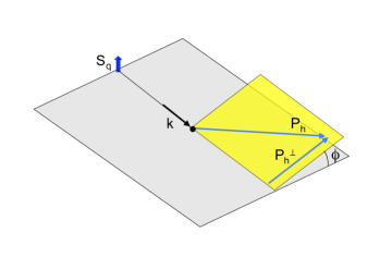
The term containing the Collins function depends on the spin vector of the quark , and introduces an azimuthal asymmetry in the distribution of hadrons around the quark three-momentum direction . The triple product of Eq. (1), in fact, produces a modulation, where is the azimuthal angle between the plane perpendicular to the quark spin, and the plane determined by and , as shown in Fig. 1. In the literature, the amplitude of this modulation is called the Collins asymmetry or the Collins effect.
Experimental evidence for a non-zero Collins function was found by the HERMES Airapetian et al. (2010); Airapetian (2005) and COMPASS Adolph et al. (2012); Alekseev (2010) collaborations, from the analysis of semi-inclusive deep inelastic scattering (SIDIS) of leptons off transversely polarized hydrogen and/or deuteron targets. The cross sections for these processes are proportional to the convolution of the Collins function and the chiral-odd transversity function Ralston and Soper (1979). The latter is the least well known among the twist-two parton distribution functions of the nucleon, and plays a crucial role in understanding the spin properties. In order to extract the transversity and the Collins functions from SIDIS data, independent measurement of at least one of them is needed.
In annihilation to a quark-antiquark pair, each quark spin is unknown:
the Collins asymmetry in a single jet () will be zero.
However, the Collins effect can be observed when the
products of the quark and antiquark fragmentation are simultaneously considered.
Experimentally, this is achieved by studying the process ,
where () is a spinless hadron ( or )
coming from the fragmenting quark ().
Events with a two-jet topology are selected, and
the correlation between the azimuthal angles of
pairs of hadrons detected in opposite hemispheres
with respect to the plane perpendicular to the jet axis is analyzed.
The resulting azimuthal asymmetry is proportional to the product of two Collins functions.
The first efforts to measure Collins asymmetries
in annihilation, by studying events,
were performed by the DELPHI Collaboration Efremov et al. (1999),
while the first observation was obtained by the Belle
Collaboration Seidl et al. (2006, 2008, 2012),
from a study of inclusive production of charged pion pairs at a
center-of-mass (c.m.) energy of approximately 10.6 .
Assuming the universality of the Collins function Metz (2002); Collins and Metz (2004),
a global analysis of SIDIS and annihilation data has been carried out
by the authors of Refs. Anselmino et al. (2007, 2009),
allowing the simultaneous extraction of the transversity and Collins functions
for the pion system.
We report the measurements of the azimuthal modulation due to the Collins effect (Collins asymmetries) in the process , where stands for charged pion and for a light quark: . We reproduce the Belle analysis Seidl et al. (2008, 2012) of the azimuthal asymmetries as a function of the pions fractional energy in two reference frames. We also perform a new measurement of the asymmetries as a function of the transverse momentum of pions with respect to the analysis axis.
II Analysis overview
Charged pions are selected in opposite jets of hadronic events according to the thrust axis of the event Brandt et al. (1964); Farhi (1977), which permits the identification of two hemispheres (called 1 and 2, respectively, along and opposite to the thrust axis direction) and to label the two pions as and . The analysis is performed in two convenient reference frames: the thrust reference frame, defined in Sec. II.1, and the second hadron momentum frame, defined in Sec. II.2. This choice follows the scheme outlined by authors of Refs. Boer et al. (1997); Boer (2009), and allows a direct comparison of our results with the Belle measurements. Section III summarizes the data sets used, while Sec. IV describes in detail the event and track selection. The analysis method is discussed in Secs. V and VI. Dilutions of the asymmetries induced by background sources and by detector effects not related to the Collins function are discussed in Secs. VII and VIII, respectively. Studies of possible systematic effects are summarized in Sec. IX, while the final results on Collins asymmetry for light quark fragmentation are reported in Sec. X.
II.1 Thrust reference frame: RF12
As mentioned in Sec. I, the Collins asymmetry manifests itself as an azimuthal modulation of two final state pions around the fragmenting quark-antiquark momentum. The direction is not accessible to a direct measurement and is approximated by the thrust axis of the event Farhi (1977). The kinematics in the c.m. system corresponding to , together with the definition of the two azimuthal angles, are schematically represented in Fig. 2. We refer to this frame as the thrust reference frame or RF12, since the thrust axis serves as reference axis for the azimuthal angles. The correlation of the quark and antiquark Collins functions in opposite hemispheres gives a product of two modulations for the azimuthal angles and , resulting in a modulation. The azimuthal angles are defined as
| (2) |
where is a unit vector defined along the direction of the electron beam,
is the thrust axis, and is
the three-momentum vector of the pion detected in the first () or in the second () hemisphere.
The differential cross section depends on the fractional energies and of the two pions,
and on the sum of the azimuthal angles and .
It can be written as Boer (2009):
| (3) |
where the summation runs over all quark flavors accessible at the c.m. energy , is the charge of the quark in units of , and the antiquark fragmentation function is denoted by a bar. The so-called transverse moments of the fragmentation functions are defined as Boer (2009):
| (4) |
with , , , and . In this equation, the pion transverse momentum has been rewritten in terms of the quark intrinsic transverse momentum 111Throughout the paper we use the subscript to denote the transverse component of a vector to the dipion axis in the frame where they are collinear, while the superscript indicates the component transverse to the axis.: , and is the pion mass.
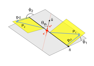
The Collins asymmetry can be extracted by measuring the cosine modulation of the distribution of the quantity on top of the uniform distribution due to the unpolarized part of the fragmentation function. Dividing the full range into one hundred intervals, we define the normalized azimuthal distribution as
| (5) |
with the di-pion yield in each subdivision, and the average bin contents.
II.2 Second-pion reference frame: RF0
The azimuthal asymmetries can also be measured in a different reference frame: following Ref. Boer et al. (1997), we use the direction of the observed pion as the reference axis, and we define the scattering plane by the beam axis and the momentum of that pion, as illustrated in Fig. 3. Also in this frame, the kinematic variables are calculated in the c.m. system, but only one azimuthal angle, , is defined:
| (6) |
We refer to this frame as the second-pion reference frame, or RF0. At leading order in the strong coupling , the differential cross section is given by Boer et al. (1997)
| (7) |
where is the transverse momentum of the virtual photon from annihilation in the frame where and are collinear Boer (2009). is a convolution integral over the transverse momenta and , with and the transverse momenta of the two fragmenting quarks:
| (8) |
and is the unit vector in the direction of the transverse momentum of the first hadron relative to the axis defined by the second hadron.
In this frame, the modulation due to the Collins effect is in the cosine of twice the azimuthal angle , and the normalized distribution is defined as
| (9) |
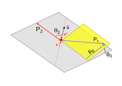
The differential cross sections in Eq. (II.1) and Eq. (II.2) for the two reference frames are related to each other. Integrating the first equation over and , and the second over and , the same unpolarized cross section is obtained. A similar relation exists for the Collins contributions. However, due to the additional convolution over the transverse momentum , the intrinsic transverse momentum dependence of the Collins function should be known to exploit it. The majority of authors assume that the Collins function is a Gaussian in , as is the unpolarized fragmentation function, with a different width from the unpolarized case. More details can be found, for example, in Refs. Anselmino et al. (2006); Bacchetta et al. (2000); Efremov et al. (2006).
II.3 Unlike, Like, and Charged pion pairs
The possibility to select pion pairs with equal or opposite charges allows sensitivity to “favored” and “disfavored” fragmentation processes. A favored fragmentation function describes the fragmentation of a quark of flavor into a hadron containing a valence quark of the same flavor: for example, and . Vice versa, we refer to and as disfavored fragmentation processes. Therefore, the production of pion pairs with opposite charge from the fragmentation of a pair () can proceed through two favored fragmentation processes ( and ) or through two disfavored fragmentation processes ( and ). Neglecting heavy quark fragmentation and introducing the favored functions , and , as well as the disfavored functions and , the cross section for charged pion pair production can be written as Efremov et al. (2006):
| (10) |
where stands for a generic charged pion, is the azimuthal angle in RF12 or in RF0, with the polar angle of the analysis axis, and the upper index indicates Unlike (U), Like (L) and Charged (C) sign pion pairs.
III BABAR experiment and data sample
The results presented here are based on a sample of data collected with the BABAR detector at the PEP-II asymmetric-energy collider, at the SLAC National Accelerator Laboratory. A total integrated luminosity of about 468 Lees et al. (2013b) is used, consisting of 424 collected at the peak of the resonance, and about 44 collected 40 below the peak.
The BABAR detector is described in detail in references Aubert et al. (2002, 2013). Charged particle momenta are measured by a combination of a 5-layer, double sided silicon vertex tracker (SVT), and a 40-layer drift chamber (DCH) that covers of the solid angle in the c.m. frame, both located inside a 1.5 T superconducting solenoidal magnet. Discrimination between charged pions, kaons, and protons is obtained from measurements of the specific ionization () in the tracking system, and from the Cherenkov light collected by an internally reflecting ring-imaging Cherenkov detector (DIRC). The DIRC covers of the c.m. solid angle in the central region of the BABAR detector and has a () identification efficiency for pions (kaons) with momenta above 222Natural units are used throughout this article. Photons and electrons are identified and their energies measured with a high resolution CsI(Tl) crystal electromagnetic calorimeter (EMC). Muons are identified in the instrumented flux return (IFR), which consists of 18 layers of steel interleaved with single-gap resistive plate chambers or limited-streamer tubes.
Detailed Monte Carlo (MC) simulation is used to test and optimize the selection criteria, to study the detector acceptance, and to estimate the contribution of various background sources. The simulation package Jetset Sjostrand (1995) is used to generate hadronic events in non-resonant annihilation. Separate MC samples are generated for light quarks, (), called generic MC, and charm quarks, . Samples of events with generic decays are generated with the EvtGen Lange (2001) package. Finally, and event samples are produced with the KK2F Ward et al. (2003) generator, and events with AfkQed Czyż et al. (2005). The generated events undergo a full detector simulation based on Geant4 Agostinelli et al. (2003) and are analyzed in the same way as the experimental data. No transverse spin effects are implemented in the MC generation, so it can be used to evaluate detector biases. In addition, the MC samples are reweighted to simulate Collins asymmetries and to study the analyzing power of the method.
IV Event and track selection
We focus on the measurement of the Collins effect in light quark fragmentation, as the helicity is conserved only in the approximation of massless quarks, and the correlation between the fragmenting quark and antiquark may be lost for heavy quarks. In this section, we summarize the event and track selection requirements.
Multi-hadronic events are selected by requiring at least three reconstructed charged particles and the value of the 2nd divided by the 0th Fox-Wolfram moment Fox and Wolfram (1979), calculated from charged tracks only, . To suppress backgrounds from , processes, and events characterized by emission of a very energetic photon via initial state radiation, we require the visible energy of the event in the laboratory frame (), defined as the sum of the energies of all reconstructed charged tracks and neutral candidates, to be higher than 7 .
Only good-quality reconstructed tracks with momenta transverse to the beam direction of at least 0.1 are considered for the asymmetry measurements. Every track is required to originate from the vicinity of the interaction point (IP) by requiring the distance of closest approach to the IP in the transverse plane cm and along the electron beam cm, and to fall within the detector acceptance region: rad, where is the polar angle of the track with respect to the beamline axis.
The thrust of the event is calculated using tracks with relaxed cuts cm and cm, as well as neutral candidates lying within the calorimeter fiducial region with an energy greater than 0.030 . To avoid possible biases originating from the different forward/backward detector configuration, the sign of the thrust axis is chosen at random.
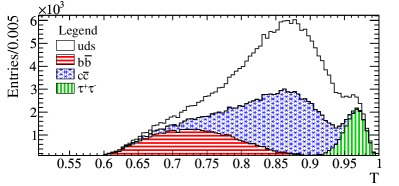
Since the correlation between the and the spin is lost in the case of emission of energetic gluons, we select the two-jet topology and suppress events by requiring a value of the event thrust . As shown in Fig. 4 the distribution of the thrust for events peaks at values higher than 0.85, but has a long tail at lower values, which is mainly due to hard gluon radiation. The requirement also removes the majority of the more spherical events produced in decays. Events with charm quarks have a shape similar to the light quarks; their contribution to the asymmetry is evaluated and subtracted as described in Sec. VII.
Events from the reaction populate the region at higher thrust values and lower , as is evident from Fig. 5, which shows a scatter plot of vs. for events having at least one good hadron pair. The small accumulation visible at lower energies and is due to events, and it is removed by applying a cut around this region, as indicated by the line in Fig. 5.
Radiative and events are the sources of the background peaking at and concentrated in particular at high . This kind of background is suppressed by requiring at least three charged hadrons in the event.
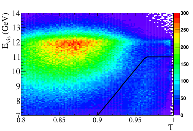
However, some events, with the initial state photon converting to a pair, can pass this selection. These events are characterized by small multiplicity and by two very energetic muons. We reduce this contamination to a negligible level by requiring that for events with multiplicity lower than five, the two most energetic tracks are not identified as muons, and no electrons are present.
Reconstructed tracks in the selected events are used for the study of the Collins asymmetries if they are identified as pions and fail to pass specific muon and electron selectors. The efficiencies estimated for the latter are about 70% and 98%, and the pion mis-identification rate of about 2% and 4%, for muons and electrons, respectively.
Two-body decays of bound states, mainly produced via initial state radiation, generate a significant amount of unlike-sign pairs, with both tracks of c.m. momentum above 4.5 . On the other hand, we expect to have very small signal from fragmentation processes with two such energetic tracks. In particular no like-sign pairs are observed in the data sample with and above 0.9. We therefore limit the study to tracks with .
The residual contributions of all other background sources (, , and ) are evaluated, and the measured asymmetry corrected as described in Sec. VII.
The fragmentation functions depend on the lightcone momentum fraction of the produced hadron with respect to the fragmenting quark Boer et al. (1997), which is equivalent to the fractional energy at large c.m. energy and not too small values of Anselmino et al. (2007),
It may be of interest to extend the study also for very low values, in order to assess when this approximation fails. On the other hand, low momentum tracks pose severe experimental difficulties due to the association of the hadrons to the incorrect jet. For these reasons, the measurement of Collins asymmetry is performed only for candidate pions with .
The selected pions are separated in opposite hemispheres according to the thrust axis (), and are combined if they satisfy the following condition
| (11) |
where are the pions momenta. For pairs with values of near to zero there is a higher probability that one of the two tracks has been assigned to the wrong hemisphere. This effect is particularly evident for pions with low fractional energies. The requirement that the pions are emitted within a cone of around the thrust axis removes the ambiguous tracks.
One of the most important contributions to azimuthal asymmetries not connected to the Collins effect originates from low energy gluon radiation , which is not completely removed by the event selection. As reported in Refs. Boer (2009); Collins (1979), the angular distribution of the gluon radiation process is given by
| (12) |
In addition, all the formalism used so far is valid in the region where the transverse momentum is small compared to () Boer (2009), and a safe compromise is to require .
The same selection is applied to same-charge and opposite-charge pion pairs. About pion pairs are selected and used in the analysis.
V Normalized azimuthal distributions
Following Eqs. (II.1) and (II.2), the azimuthal distributions of the normalized yields , defined in Sec. II, can be parametrized as
| (13) |
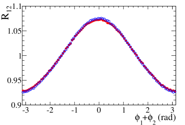
where indicates the reference frame, the charge combination of the pion pair, and is the azimuthal angle combination or , according to the frame used. The parameter should be consistent with unity, while gives the amplitude of the asymmetries. The normalized azimuthal distributions, presented in Fig. 6 for MC and data samples, are strongly affected by detector acceptances and show apparent modulations. This is clearly visible in the simulated sample, for which a flat distribution is expected since the polarized are not implemented in the MC generator. However, the and distributions are almost coincident in the MC sample (Fig. 6(a)), while a clear difference is observed in data (Fig. 6(b)). This difference is the observable effect of the azimuthal asymmetry produced by the Collins effect.
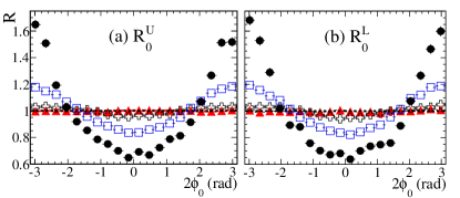
Detector effects depend on the jet direction. When the pair is created at low polar angle with respect to the beam axis, there is a higher probability that part of the jet falls outside the detector coverage, and the thrust can be badly reconstructed. The result is a distortion of the distribution, as visible in Fig. 7, which shows and in the RF0 frame for different intervals of . The same effect is also visible in the RF12 frame. The triangles in Fig. 7 also show the residual effects of gluon radiation to be small. We can parameterize the acceptance effects on the normalized distribution as an additional contribution to the modulation, whose amplitude varies with : . Therefore, Eq. (13) becomes:
| (14) |
and shows a coupling between the Collins and detector acceptance effects proportional to .
In principle, it would be possible to estimate detector acceptance effects with simulated events, and correct the asymmetries measured in the data sample, but this procedure would introduce large uncertainties. All these considerations suggest the possibility to form a suitable double ratio of azimuthal distributions, in order to reduce the effect of detector acceptance and perform a measurement almost independent from simulation.
VI Double ratios
Given the difficulties in separating the Collins effect from asymmetries produced by detector acceptances and radiative effects, we exploit the fact that most of the instrumental effects should largely cancel in ratios of asymmetries, as for example, the ratio of unlike-sign over like-sign asymmetries:
| (15) |
Here, and are, respectively:
| (16) |
where we omitted the and dependence in order to simplify the notation. The double ratio (DR) is performed after the integration over the polar angle , so that the average values of the quantity appear. These average values do not differ for like-, unlike- and all charged-pion pairs. In Eq. (15) we assume that the detector acceptance effects do not depend on the charge combination of the pion pairs, that is . We also neglect the extra term proportional to , which couple the detector acceptance to the true Collins asymmetries, and stop the series expansion at the first order in . We have checked for the presence of these and other terms in addition to the modulation and found them negligible. Also the assumption of acceptance effects independent on the charge combination of the pion pairs seems to hold, and noting that also the asymmetries produced by gluon radiation do not depend on the charge combination, the asymmetry amplitudes resulting from the double ratio should mainly depend on a different combination of favored and disfavored fragmentation functions (see also discussion in Sec. IX).
Similarly, the DR of the normalized distributions of unlike-sign and charged pion pairs is given by:
| (17) |
with
| (18) |
The measured U/L and U/C double ratios can be used to derive information about the relative sign and magnitude of favored and disfavored fragmentation functions Efremov et al. (2006). Analogous expressions can be obtained in the RF0 reference frame, with modulations in instead of .
The DRs are still parametrized by a cosine function
| (19) |
where and are free parameters. The constant term should be consistent with unity and the parameter , which depends on , pt, and the average value of , should mainly contain the Collins effect.
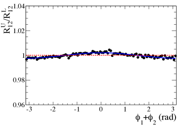
Figure 8 shows the DR of unlike to like sign pion pairs for samples of simulated and data events. The distribution for the MC sample is now essentially flat as expected; however, a slight deviation from zero asymmetry, of the order of 0.2%, is measured. The origin and the effect of this bias will be discussed in Sec. IXa. A clear cosine modulation is instead visible in the data sample (Fig. 8(b)), which can be attributed to the Collins effect.
Thanks to the large amount of data, we can study the dependence of the asymmetry as a function of fractional energies ( and ) and transverse momenta ( and , and ) of the selected pions. We choose ()-bins, with the following intervals: , , , , , ; we use () bins in the RF12 frame, and 9 bins in the RF0 frame. The intervals are defined in Tab. 3.
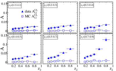
Figure 9 shows the asymmetries obtained from fits to the UL double ratio () in the RF12 frame for data and MC samples in every bin. The asymmetries are not corrected for the effects described in the next three sections, and report only the statistical errors. Similar results are obtained for the asymmetries measured in the RF0 frame, and as a function of pion transverse momenta.
VII Contribution of background events to the asymmetries.
The presence of background processes modifies the measured asymmetry . This is obtained by fitting the double ratio of the selected sample, and can be written as:
| (20) |
Here, , is the true Collins asymmetry produced by the fragmentation of light quarks, while and are, respectively, the asymmetry and the fraction of pion pairs in the selected sample due to the background component.
The background processes giving a significant contribution after the selection procedure are , , and . We refer to them as the , charm and bottom backgrounds, respectively. In the former process, azimuthal asymmetries can arise from parity violation in the weak decay of the heavy leptons. For charm processes the Collins effect is expected to be suppressed by the heavy mass of the fragmenting quarks. The study of the azimuthal asymmetries for processes would be interesting on its own, but larger data samples and an optimized analysis would be necessary to perform precise measurements. No asymmetries arising from the Collins effect are expected from decays.
The fractions and the asymmetries of the background components are determined using both MC and data control samples specific to each process, and evaluated for each bin of and .
The background
In order to assess whether a significant asymmetry is produced by processes we study a -enhanced data sample, consisting of the events in the lower-right side of the -vs.- distribution of Fig. 5, and rejected by the cut shown in the same picture. The purity of this control sample is estimated to be about ; the fitted asymmetries are very small and consistent with zero within about two standard deviations. We also perform the analysis on a sample of simulated events, applying the same event selection as for the data, and obtain asymmetries consistent with the small bias observed in the MC sample.
The contribution of the background appears in Eq. (20) as the product of the asymmetry multiplied by the pion pairs fraction . We estimate from the number of pion pairs selected in a MC sample of events scaled by the data/MC luminosity ratio, independently for every and bin. The values of range from about at low , to more than at high , and are around independently of .
Considering that the asymmetries measured in the -enhanced samples are consistent with zero or give only very small deviations from zero, and that the contamination from events is significant only at large , where the Collins effect from is large (see Fig. 9), we set everywhere.
The and backgrounds
The fraction of pion pairs due to events is much larger than the component, because of the higher production cross section and of event shapes similar to those for light quark production. The fraction , estimated with a generic -MC sample, amounts to about 25% for the whole data sample, roughly independent of , but ranging from about 30% for pairs with low fractional energies down to less than one percent at the highest values.
The events are strongly suppressed by the event selection, mainly because of the cut on the event thrust, and the fractions are estimated to be at most 2% for low fractional energies, with no tracks with . As a consequence even a sizable asymmetry in the sample would have negligible effect on the measured asymmetry, and we set .
On the contrary, given the large fractions, the azimuthal asymmetries of the selected charm sample, even if small, can have a significant impact on the total asymmetries, and therefore have to be independently measured. For this purpose, we select a charm-enhanced data sample requiring at least one candidate from the decay , with the candidate reconstructed in the following Cabibbo-favored decay channels: , , , and . Note that a control sample built in this way will contain also a fraction of events.
The reconstructed mass is required to be within of the world average value Beringer et al. (2012). A low momentum pion is then combined with the candidate in order to obtain the candidate. We retain events with at least one candidate for which , where is the mass difference between the reconstructed and candidates.
As for the full data sample, we measure the azimuthal asymmetry by fitting the double ratio of pion pair distributions in the -enhanced control sample. The estimated fractions of pion pairs in this sample that are from events average about , with values for the individual -bins ranging from more than to about with decreasing fractional energies, and almost constant with . Fractions from events amount to a few percent at low energies, and vanish for .
Corrections to the measured asymmetries
Using the asymmetries and fitted respectively in the full and -enhanced data samples, together with the fractions and , and assuming and that the charm asymmetry is the same in both samples, we can write
| (21) |
The unknown background-corrected Collins asymmetries and the charm contribution are obtained solving these equations in each bin of and .
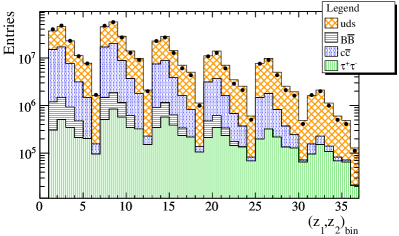
A significant source of systematic error in this procedure can arise from the fractions and , which are estimated with MC simulation. The cross sections in processes are known at no better than the few percent level; furthermore, only a fraction of all charmed-hadrons and -meson decays have been measured and included in the EvtGen generator. Also decays with many hadrons in the final state are known with significant uncertainties only. In order to evaluate the effect of these uncertainties on the measured fractions, we compare bin-by-bin the number of pion pairs selected in the data with those selected in the , , charm, and bottom MC samples, summed according to the nominal production cross sections. The observed data-MC differences are at most at the few percent level as can be deduced by Fig. 10. Conservatively, we assign these differences as additional uncertainties on the charm (, and ) and tau () fractions, which are the most significant contributions in the extraction of and from Eq. (21). This choice has a very little effect on the final result, given that the uncertainties on the background subtraction procedure are dominated by the statistical errors of the fit to the control sample, in particular for bins of high fractional energies.
We check the consistency of the -enhanced sample by performing the correction of the measured asymmetries, and the estimation of the charm contributions independently for the four decay modes, finding no significant differences.
VIII Asymmetry dilution due to detector effects
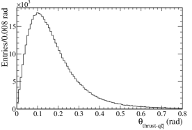
The experimental method uses the thrust axis to estimate the axis. The distribution of the opening angle between the two axes for simulated events, shown in Fig. 11, peaks at about 100 mrad, and has a long tail at higher values. This produces a dilution of the asymmetries, in particular in the thrust reference frame, where the azimuthal angles and are calculated with respect to the thrust axis (see Fig. 2). The impact on the measurement of the azimuthal angle in RF0 is small. Particle identification and tracking resolution have small effects in both frames.
An additional smearing of the azimuthal angles can occur when the track is very close to the analysis axis, where a small mis-measurement of the track results in a large shift in the azimuthal angle. A larger effect is expected in RF12 where, by construction, energetic tracks are close to the thrust axis.
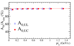
These and other detector effects can be studied via MC simulation, comparing the fitted asymmetries with those introduced in the simulation. The MC generator does not include the Collins effect, so we remodulate the generated azimuthal distributions applying to every selected pion pair a weight defined as with and or . In RF12 the angle is the sum of the azimuthal angles and for generated particles calculated with respect to the true quark-antiquark axis, while in RF0 the angle is calculated with respect to the 3-momentum of one of the generated pions which makes the pair. The ratio of the fitted to the simulated asymmetry should be unity for perfect reconstruction, i.e. if all , where are the proper combinations of azimuthal angles in the reconstructed MC sample. We verify that for the fitted asymmetry is consistent with the biases observed in Sec. VI. We consider several values between zero to 0.1, independent of , and . Subtracting the bias and taking the ratio for each, we obtain dilution values that vary by less than their statistical error in each , , and bin. We therefore average these values in each bin and use them to correct the background-corrected data.
As shown in Fig. 12(a), the results for RF0 are essentially consistent with the simulated asymmetries for every bin. On the contrary, the fitted asymmetries for RF12 (Fig. 12(b)) systematically underestimate the generated values, with correction factors ranging from about 1.3 to 2.3 with increasing values of , and from about 3 to 1.3 with increasing values of . The errors on weighted averages of the correction factors are assigned as systematic errors.
Collins asymmetries are expected to depend on the polar angle of the analysis axis, as well as on the two pions’ and , and any strongly dependence might affect the dilution factors. We have evaluated these factors using weights in which has the expected linear dependence on the quantity , and weights that contain a linear combination of , such as . The measured dilutions are in good agreement each other and the shifts in the values are within the uncertainties. Since from the results of the tests performed there are no indications of the dependence of the dilution on the true asymmetry, we report the results using uniform weighting.
IX Study of systematic effects
We have identified a number of systematic effects that can potentially influence the measurement of the asymmetries. The sizable effects are corrected as described above; here we discuss the origins and uncertainties of these and other effects. Unless otherwise stated, all the systematic uncertainties are evaluated in each bin.
Test of the DR method on Monte Carlo sample.
The MC generator describes the radiative gluon effects, but does not contain asymmetries based on the Collins effect. Nevertheless, as discussed in Sec.VI and visible in Fig. 9, the fitted asymmetries for the -MC samples show deviations from zero at all values of the pion transverse momenta and fractional energies. The fitted asymmetries are small with respect to the data everywhere, but not negligible in several cases, being of the same order as other systematic uncertainties. In order to understand the origin of this bias we compare three different MC samples: the first sample is built at generator level, that is taking the momenta of pions as produced by the event generator; the second sample also uses generator level momenta, but only pions with associated reconstructed and identified tracks; the last sample is the standard fully reconstructed MC sample. We also compare the results using as reference axis the true axis, instead of the thrust axis, and varying the criteria that define the track detector acceptance, as track polar angle and number of hits per track in the DCH. As a result of these investigations we conclude that the small bias observed in RF0 is due to a non-perfect cancellation of the detector effects in the double ratio procedure, while in RF12 the main effects come from the use of the thrust axis as a reference axis. We subtract the estimated bias from the asymmetry, and take as systematic uncertainty the combination in quadrature of the largest variation of the performed tests with the statistical error of the bias measured with the standard fit.
Uncertainties due to the resolution.
The Collins effect also depends on the pion momentum transverse to the direction of the fragmenting quark (, as in Fig. 1). In the RF12 frame, this quantity is not accessible because the momenta of the fragmenting quarks is not known, and the asymmetries are measured as a function of the momenta of the pions transverse to the thrust axis ( and ). In order to convert the measured asymmetries to the asymmetries with respect to the true momenta, one must account not only for the dilution effect discussed in the prevoius section, but also for the migration of pion pairs from one momentum-bin to another. The resolution function is obtained for different ranges making use of the MC sample. We fit the distribution of the difference between the true and the reconstructed transverse momentum with a double gauss function, or a crystal-ball function for ; the width of the dominant gaussian component results of the order of 100 . These resolution functions are then used to redistribute the pion pairs in the various bins according to the probability that they were generated in that particular bin, and the fit to the azimuthal distributions of the new bin contents are performed. The relative difference between the asymmetries obtained with this and the standard procedure are of the order of 10% for every bin, with the exception of the lower bin, were it amounts to about 30%; these differences are assigned as systematic uncertainties.
Uncertainties due to particle identification.
With the algorithm used, the probability of misidentifying kaons and protons as pions has been measured to be a few percent per track. This results in a purity for the selected pion pair sample of about , with the remaining of pairs made of a true pion and a true kaon. We repeat the study with both more stringent and more loose selection criteria, and compare the results with the standard selection. Good agreement is found among the different selections; the absolute values of the differences amount to at most a few percent of the measured asymmetries and are assigned as systematic errors.
Uncertainties due to the fit procedure.
The dependence of the measured asymmetries on the binning
is checked by comparing the results with three different
bin sizes of the azimuthal angles and :
, , and (used for the standard analysis).
The largest deviations are less than 1% and are taken as systematic errors.
The DR distributions are fitted by Eq. 19, which approximates
the series expansion to the first order in ,
with the azimuthal angles in the respective reference frame and ,
and neglects possible contribution due to the
detector acceptance.
In order to check for the sensitivity to these contributions,
we use different fitting functions with additional higher harmonic terms.
No significant changes in the values of the cosine moments
with respect to the standard fits are observed.
A certain level of correlation among the entries of the double ratio
distributions is expected because the same pion can be used to form
several pion pairs, so that the statistical error returned by the
fits could be underestimated.
We check for this effect, performing a set of 3000 pseudo-experiments.
For each pseudo-experiment we randomly generate according to
the fit model a statistical sample of the same size of that selected by
the analysis procedure.
Gaussian fits to the pull distributions of the values of the fitted
asymmetries give results consistent with a vanishing mean
and a unit width, as expected for an unbiased fit model.
Test of the double ratio with same sign pion pairs.
The Collins effect does not depend on the electric charge, but only on the combination of favored and disfavored fragmentation functions in the particular charge combination of the paired pions. In particular, the same combination appears when a or a pair is considered. Gluonic radiative effects do not depend on the electric charge either. Therefore, we can test the double ratio procedure and the possible charge dependence of the detector response by probing the ratio of normalized azimuthal distributions for positively charged over negatively charged pion pairs. Results consistent with unity are obtained.
Subtraction method and double ratio.
As a cross check of the double ratio method we also extract the asymmetry by using a different procedure which consists of taking the difference, instead of the ratio, of pion pair rates. In this case, gluon radiation effects cancel at all orders, while the cancellation of the acceptance effects could be non optimal. The asymmetries measured with the two methods are consistent, making us confident that possible radiative and detector effects not canceling in the double ratio procedure do not significantly affect the results.
Study of beam polarization effects.
Charged particles circulating in a magnetic field become polarized transverse to the beam direction due to the emission of spin-flipping synchrotron radiation, known as the Sokolov-Ternov effect Sokolov and Ternov (1964). Beam polarization can affect the angular distribution of produced hadrons in introducing an azimuthal asymmetry with respect to the beam spin direction. This asymmetry has in common with the Collins asymmetry that both are transverse single spin asymmetries: the former concerning lepton spins, the latter quark spins. The beam polarization is expected to be negligible at the PEP-II interaction point. This can be verified by studying the reaction , whose cross section can be written as Learned et al. (1975):
| (22) |
where is the degree of transverse polarization of the beams, and and are the polar and azimuthal angles of the produced muons in the center of mass system.
We analyze the and distributions of selected muon pairs, emitted at a polar angle , in order to ensure that they fall within the SVT coverage. We perform the fit to the whole sample and separately to the samples corresponding to the different data taking periods. In all cases the fits are consistent with expectations for unpolarized beams. We conclude that no significant systematic errors need to be assigned for possible buildup of beam polarization.
Consistency of asymmetries in different data sets.
The results reported in this paper are obtained combining the data taken at two different c.m. energies, at the peak of the resonance and 40 below. While the slightly different energy is not a problem, the two sets of data differ for the background due to . We perform a consistency check of the results obtained fitting separately the two data sets ( and ) as follows:
| (23) |
with the summation over or bins, and the statistical error on the measured asymmetry . We find the overall per degree of freedom ranging between 1.2 and 0.7. Analogous checks performed on sub-samples of data collected in different data-taking periods show a general consistency of the results.
Summary of systematic uncertainties.
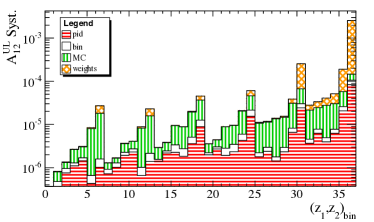
All systematic effects are evaluated for each bin of fractional energy and pion transverse momentum. As an example, the sizable contributions to the absolute systematic errors for are shown as a function of the 36 () bins in Fig. 13(a), and as a function of the 16 () bins in Fig. 13(b). The histograms report the squared errors assigned for uncertainties due to particle identification (pid), bin size of the azimuthal distributions (bin), estimate of the bias observed in the MC sample (MC), and estimate of the correction factors for the dilution of the asymmetry (weights). The two latter sources dominate at high fractional energies, while at low- values all contributions are comparable. In Fig. 13(b) is also reported the squared uncertainty due to the resolution (res). This, and the uncertainty in the estimate of the bias are the dominant sources at all values of transverse momenta in the RF12 frame. The total systematic error is obtained by adding in quadrature the individual contributions.
The contribution of the various background sources (, , and events) to the measured asymmetries is subtracted with the procedure described in Sec. VII. Through Eq. (21), the statistical error of the Collins asymmetries account for the statistical uncertainties of the asymmetries measured in the full and in the -enhanced data sample, and for the statistical and systematic uncertainties in the determination of the relative fractions and .
X Results
This section summarizes the measured asymmetries as a function of fractional energies , transverse momenta , and polar angle of the analysis axis, after all corrections and systematic uncertainties discussed in the previous sections are applied. We also report the asymmetry measured in RF12 in a four-dimensional space, as a function of ().
X.1 Collins asymmetries vs. fractional energies
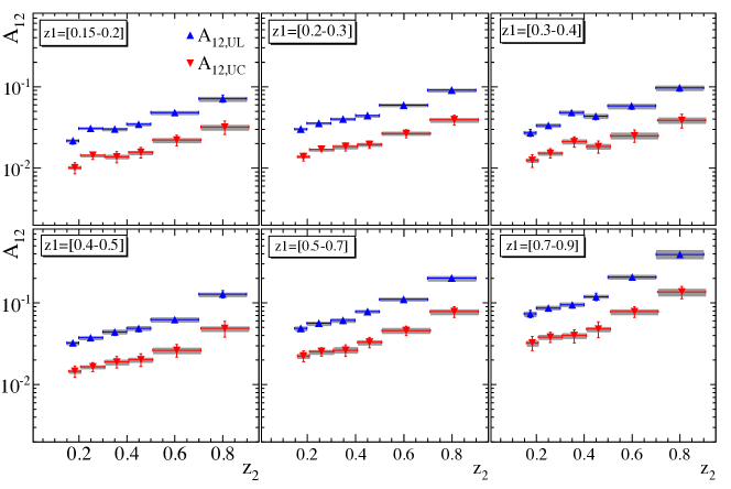
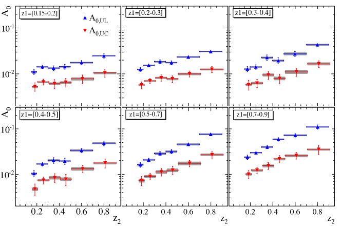
The Collins asymmetries measured for each bin are summarized in Tabs. 1 and 2, and illustrated in Fig. 14 and Fig. 15, for RF12 and RF0, respectively. In each plot the asymmetries are reported for every bin in a given interval of . We note a very good consistency among symmetric bins, with and exchanged, giving additional confidence on the correctness of the fitting procedure. A rise of the asymmetries with increasing pion energies is clearly visible in all plots, in agreement with theoretical predictions Bacchetta et al. (2001, 2008); Buttimore et al. (2001) and Belle results Seidl et al. (2008, 2012). The measured values span more than an order of magnitude, being about 1-2% in the lower bins, and close to 40% for at the highest energies.
The measured UC asymmetries are smaller than the UL asymmetries by roughly a factor of 2. This behavior was already observed by Belle, and should reflect the different contribution of favored and disfavored fragmentation functions to the UC and UL ratios, as discussed in Sec. VI. An analysis of Belle data, under the assumption
| (24) |
found values for the parameters and consistent with a large disfavored Collins fragmentation function with sign opposite to the favored one Efremov et al. (2006), as also suggested by the HERMES experiment Airapetian (2005).
X.2 Collins asymmetries vs. transverse momenta
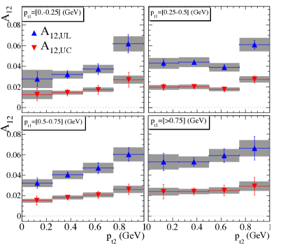
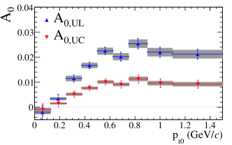
The Collins asymmetries measured in the two reference frames, in bins of and , are shown in Fig. 16 and Tab. 3. The results from the two double ratios are reported. This is the first measurement of the dependence on the pion transverse momenta in annihilation, and is important for a theoretical understanding of the evolution of the Collins fragmentation function. In RF0 the measured asymmetries are consistent with zero at very low , rise almost linearly up to about 2% for UL and 1% for UC, at 0.8 , and then flat. In RF12 the asymmetries slightly differ from zero at low transverse momenta, and exhibit also in this case a smooth rise of the asymmetries with up to a maximum of about 7% and 3% for UL and UC, respectively. Due to the limited resolution at very low transverse momenta it is not possible to verify the expected vanishing of with going to zero. The average value for the lowest bin is, in fact, .
X.3 Collins asymmetries vs. and
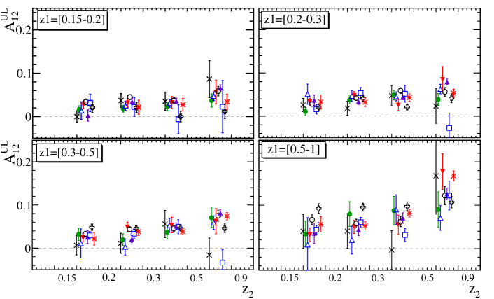
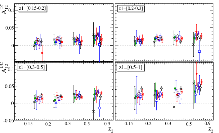
The study of the asymmetry behavior as a function of both pion fractional energies and transverse momentum is an important test to probe the factorization of the Collins fragmentation function assumed in Ref. Anselmino et al. (2007) and, in general, provides a powerful tool to access correlations in the Collins asymmetries. We perform this study in the thrust reference frame, using four and three () intervals. The boundaries for the fractional energies intervals are set to and , while the intervals for the transverse momenta are , , and . We estimate background contributions, dilution effects, and systematic uncertainties independently for each bin, following the procedures described in the previous sections. The results are summarized in Tabs. 4, 5 and 6, and in Fig. 17.

X.4 Collins asymmetries vs. polar angles
The transverse polarization of the original pair created in annihilation should be proportional to , where is the polar angle of the axis with respect to the beam axis. The Collins asymmetry should manifest a similar dependence, as shown by Eqs. (15) and (17) for the UL and UC ratios, respectively. We can test this prediction, and in particular that the asymmetries vanish for , by studying the asymmetries as a function of the quantity after integration over and , with the polar angle estimated by the polar angle of the thrust axis () or of the reference hadron ().
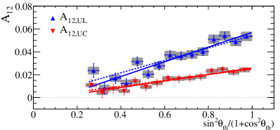
The results are displayed in Fig. 18 and summarized in Tab. 7. The asymmetries are corrected for background contributions and dilution effects, following the same procedure described in Secs. VII and VIII. As systematic uncertainties we assigned the average values of the significant contributions studied in Sec. IX, which are added in quadrature in Fig. 18 (gray error bands).
We subject each set of data points to a linear fit (), both with the intercept parameter floating and constrained to the origin of the axes (). The results of these fits are summarized in Tab. 8. For , all four fits have a good , and both fitted are consistent with zero (Fig. 18(a)). Also the asymmetries are consistent with a linear dependence on , but the results clearly favor a non zero constant term for both and (Fig. 18(b)). This behavior is in contradiction with the cross section formula reported in Eq. II.2, the origin of which is not understood.
XI Summary
We have presented a set of measurements of azimuthal asymmetries in inclusive production of charged pion pairs in annihilation, where the two pions arise from the fragmenting quarks in opposite jets. We consider two reference frames, and extract asymmetries from suitable ratios of normalized azimuthal distributions: the ratio of opposite-sign to same-sign pion pairs (UL double ratio) and the ratio of opposite-sign to any charge pion pairs (UC double ratio). We observe clear, non-vanishing asymmetries that can be related to the Collins fragmentation functions.
We measure the Collins asymmetries as a function of several variables, including the transverse momenta ( and , and ) of the pions with respect to the analysis axis, their fractional energies , and polar angle of the analysis axis with respect to the beam axis.
The asymmetries rise with and , as expected from theoretical predictions, and span more than an order of magnitude. Our data are also consistent with the previous measurements performed by the Belle Collaboration Seidl et al. (2006, 2008), with the exception of the bins where the highest fractional energies are involved. In particular we measure an asymmetry about three standard deviations higher in the highest () bin. It must be noted, however, that the two data sets are not directly comparable, because of the different width of the highest interval, which is for Belle, while we limit our study to for the reasons explained in Sec. IV.
Theoretical calculations with different approaches have been proposed to make predictions or to reproduce the available data (see for example Refs. Efremov et al. (2006); Bacchetta et al. (2008) and references therein). The new precise data presented here can be used to improve the tuning of the various models and possibly discriminate among the different assumptions. These results can also be combined with Belle and SIDIS data to improve the simultaneous extraction of favored and disfavored , and the transversity and other chiral-odd parton distributions, following, e.g., the approach of Ref. Anselmino et al. (2007, 2009).
There is an increase of the asymmetries with increasing , more pronounced in the RF0 system, and there is an indication that a maximum value of the asymmetry is reached at . The available data sample is not sufficient to effectively study the region above 1 , and determine if the asymmetries decrease after the peak is reached. No previous data from annihilation are available to compare with. Assuming that the evolution333In SIDIS processes is the 4-momentum transferred from the lepton to the struck hadron, while in annihilation it is equal to s. of the Collins function is the same as for the unpolarized function, the authors of Ref. Anselmino et al. (2007) extracted the dependence at . However, such an assumption on the evolution with is not established, and even questionable, given the chiral-odd nature of the Collins function. Alternative choices have been proposed, including the extreme case that the Collins function does not evolve with the energy scale Bacchetta et al. (2008). The measurement of the asymmetry as a function of obtained by BABAR at , that is an energy scale much higher with respect to the data presently available from SIDIS, will be very valuable in shedding light on this important question.
We also measured the asymmetries in bins of the quantity , where is or according to the reference frame used, as defined in Fig. 2 and Fig. 3, respectively. The expected linear dependence is observed in both reference frames. However in RF0 the fit result is inconsistent with a line crossing the origin, in disagreement with expectations.
XII ACKNOWLEDGMENTS
The authors would like to thank Ralf Seidl of the Belle
Collaboration for the fruitful discussions on the analysis method.
We are also grateful to Mauro Anselmino and Marco Contalbrigo,
for the helpful discussions on the theoretical aspects of the measurement.
We are grateful for the extraordinary contributions of our PEP-II colleagues in
achieving the excellent luminosity and machine conditions
that have made this work possible.
The success of this project also relies critically on the
expertise and dedication of the computing organizations that support BABAR.
The collaborating institutions wish to thank
SLAC for its support and the kind hospitality extended to them.
This work is supported by the US Department of Energy
and National Science Foundation, the
Natural Sciences and Engineering Research Council (Canada),
the Commissariat à l’Energie Atomique and
Institut National de Physique Nucléaire et de Physique des Particules
(France), the Bundesministerium für Bildung und Forschung and
Deutsche Forschungsgemeinschaft (Germany), the
Istituto Nazionale di Fisica Nucleare (Italy),
the Foundation for Fundamental Research on Matter (The Netherlands),
the Research Council of Norway, the Ministry of Education and Science of the Russian Federation,
Ministerio de Economía y Competitividad (Spain), and the
Science and Technology Facilities Council (United Kingdom).
Individuals have received support from the Marie-Curie IEF program (European Union) and the A. P. Sloan Foundation (USA).
| (%) | (%) | ||||||||||
|---|---|---|---|---|---|---|---|---|---|---|---|
| (GeV) | (GeV) | (GeV) | |||||||||
| 0.174 | 0.308 | 0.174 | 0.307 | 0.372 | 0.716 | 0.687 | 2.16 0.20 0.09 | 1.11 0.14 0.05 | |||
| 0.174 | 0.310 | 0.244 | 0.369 | 0.364 | 0.715 | 0.683 | 3.07 0.18 0.12 | 1.43 0.12 0.05 | |||
| 0.174 | 0.313 | 0.344 | 0.431 | 0.356 | 0.711 | 0.676 | 2.99 0.27 0.16 | 1.34 0.16 0.06 | |||
| 0.174 | 0.315 | 0.444 | 0.475 | 0.351 | 0.706 | 0.671 | 3.42 0.28 0.17 | 1.44 0.17 0.06 | |||
| 0.174 | 0.318 | 0.577 | 0.506 | 0.346 | 0.697 | 0.663 | 4.77 0.39 0.29 | 1.76 0.20 0.07 | |||
| 0.174 | 0.322 | 0.772 | 0.439 | 0.339 | 0.683 | 0.655 | 7.02 0.71 0.50 | 2.48 0.26 0.08 | |||
| 0.244 | 0.369 | 0.174 | 0.309 | 0.511 | 0.715 | 0.685 | 2.99 0.18 0.11 | 1.24 0.12 0.05 | |||
| 0.244 | 0.372 | 0.244 | 0.372 | 0.490 | 0.713 | 0.682 | 3.55 0.18 0.13 | 1.53 0.11 0.06 | |||
| 0.244 | 0.376 | 0.344 | 0.435 | 0.467 | 0.710 | 0.676 | 3.99 0.27 0.19 | 1.83 0.17 0.06 | |||
| 0.244 | 0.378 | 0.444 | 0.479 | 0.453 | 0.706 | 0.672 | 4.38 0.27 0.20 | 1.76 0.17 0.06 | |||
| 0.244 | 0.380 | 0.577 | 0.511 | 0.438 | 0.698 | 0.665 | 5.93 0.36 0.30 | 2.32 0.19 0.08 | |||
| 0.244 | 0.379 | 0.772 | 0.442 | 0.412 | 0.685 | 0.658 | 8.98 0.65 0.49 | 3.07 0.24 0.08 | |||
| 0.344 | 0.430 | 0.174 | 0.311 | 0.707 | 0.710 | 0.682 | 2.69 0.27 0.17 | 1.27 0.16 0.06 | |||
| 0.344 | 0.434 | 0.244 | 0.375 | 0.661 | 0.710 | 0.680 | 3.34 0.25 0.20 | 1.41 0.16 0.06 | |||
| 0.344 | 0.438 | 0.344 | 0.438 | 0.613 | 0.706 | 0.674 | 4.80 0.42 0.31 | 2.26 0.31 0.12 | |||
| 0.344 | 0.440 | 0.444 | 0.482 | 0.580 | 0.702 | 0.671 | 4.33 0.41 0.30 | 1.95 0.29 0.11 | |||
| 0.344 | 0.439 | 0.577 | 0.515 | 0.548 | 0.696 | 0.665 | 5.71 0.53 0.45 | 2.74 0.32 0.18 | |||
| 0.344 | 0.433 | 0.772 | 0.442 | 0.493 | 0.684 | 0.659 | 9.62 0.93 0.71 | 4.31 0.35 0.22 | |||
| 0.444 | 0.475 | 0.174 | 0.313 | 0.901 | 0.706 | 0.680 | 3.21 0.27 0.19 | 1.03 0.17 0.06 | |||
| 0.444 | 0.479 | 0.244 | 0.377 | 0.828 | 0.706 | 0.678 | 3.70 0.25 0.21 | 1.69 0.17 0.06 | |||
| 0.444 | 0.483 | 0.344 | 0.439 | 0.752 | 0.702 | 0.673 | 4.40 0.41 0.30 | 2.04 0.29 0.11 | |||
| 0.444 | 0.484 | 0.444 | 0.483 | 0.699 | 0.699 | 0.669 | 4.87 0.47 0.31 | 1.96 0.31 0.11 | |||
| 0.444 | 0.481 | 0.578 | 0.516 | 0.647 | 0.693 | 0.664 | 6.20 0.57 0.46 | 3.36 0.34 0.20 | |||
| 0.445 | 0.471 | 0.774 | 0.441 | 0.564 | 0.681 | 0.659 | 12.62 1.36 0.82 | 4.84 0.51 0.24 | |||
| 0.577 | 0.506 | 0.174 | 0.315 | 1.155 | 0.697 | 0.677 | 4.81 0.39 0.33 | 1.62 0.20 0.10 | |||
| 0.577 | 0.510 | 0.244 | 0.379 | 1.042 | 0.698 | 0.675 | 5.55 0.36 0.34 | 2.07 0.19 0.10 | |||
| 0.577 | 0.514 | 0.344 | 0.438 | 0.921 | 0.696 | 0.671 | 6.09 0.55 0.37 | 2.85 0.32 0.19 | |||
| 0.578 | 0.514 | 0.444 | 0.481 | 0.840 | 0.693 | 0.667 | 7.82 0.60 0.39 | 3.17 0.34 0.19 | |||
| 0.579 | 0.515 | 0.579 | 0.515 | 0.769 | 0.688 | 0.662 | 10.97 0.73 0.62 | 4.57 0.37 0.25 | |||
| 0.580 | 0.508 | 0.775 | 0.440 | 0.653 | 0.675 | 0.656 | 19.80 1.50 1.57 | 7.66 0.62 0.31 | |||
| 0.772 | 0.437 | 0.174 | 0.319 | 1.515 | 0.683 | 0.672 | 7.28 0.75 0.55 | 2.37 0.26 0.11 | |||
| 0.772 | 0.442 | 0.244 | 0.379 | 1.314 | 0.685 | 0.672 | 8.67 0.62 0.56 | 2.99 0.24 0.11 | |||
| 0.773 | 0.443 | 0.344 | 0.433 | 1.111 | 0.684 | 0.668 | 9.52 0.88 0.61 | 4.00 0.35 0.20 | |||
| 0.774 | 0.442 | 0.445 | 0.469 | 0.978 | 0.682 | 0.665 | 11.92 1.29 0.69 | 5.91 0.52 0.24 | |||
| 0.775 | 0.440 | 0.580 | 0.506 | 0.869 | 0.676 | 0.659 | 20.73 1.59 1.41 | 7.26 0.61 0.30 | |||
| 0.776 | 0.458 | 0.776 | 0.461 | 0.735 | 0.664 | 0.651 | 39.31 3.26 5.06 | 11.10 1.19 0.39 |
| (%) | (%) | ||||||||||
|---|---|---|---|---|---|---|---|---|---|---|---|
| (GeV) | (GeV) | (GeV) | |||||||||
| 0.174 | 0.308 | 0.174 | 0.307 | 0.372 | 0.716 | 0.687 | 1.01 0.16 0.05 | 0.52 0.11 0.03 | |||
| 0.174 | 0.310 | 0.244 | 0.369 | 0.364 | 0.715 | 0.683 | 1.41 0.15 0.06 | 0.66 0.10 0.03 | |||
| 0.174 | 0.313 | 0.344 | 0.431 | 0.356 | 0.711 | 0.676 | 1.37 0.22 0.09 | 0.61 0.14 0.04 | |||
| 0.174 | 0.315 | 0.444 | 0.475 | 0.351 | 0.706 | 0.671 | 1.54 0.23 0.09 | 0.65 0.14 0.04 | |||
| 0.174 | 0.318 | 0.577 | 0.506 | 0.346 | 0.697 | 0.663 | 2.19 0.33 0.16 | 0.78 0.17 0.06 | |||
| 0.174 | 0.322 | 0.772 | 0.439 | 0.339 | 0.683 | 0.655 | 3.16 0.61 0.26 | 1.05 0.21 0.06 | |||
| 0.244 | 0.369 | 0.174 | 0.309 | 0.511 | 0.715 | 0.685 | 1.38 0.15 0.06 | 0.57 0.10 0.03 | |||
| 0.244 | 0.372 | 0.244 | 0.372 | 0.490 | 0.713 | 0.682 | 1.67 0.14 0.07 | 0.70 0.09 0.03 | |||
| 0.244 | 0.376 | 0.344 | 0.435 | 0.467 | 0.710 | 0.676 | 1.81 0.21 0.10 | 0.82 0.13 0.04 | |||
| 0.244 | 0.378 | 0.444 | 0.479 | 0.453 | 0.706 | 0.672 | 1.94 0.21 0.10 | 0.77 0.13 0.04 | |||
| 0.244 | 0.380 | 0.577 | 0.511 | 0.438 | 0.698 | 0.665 | 2.65 0.30 0.16 | 1.00 0.15 0.06 | |||
| 0.244 | 0.379 | 0.772 | 0.442 | 0.412 | 0.685 | 0.658 | 3.86 0.55 0.26 | 1.25 0.19 0.06 | |||
| 0.344 | 0.430 | 0.174 | 0.311 | 0.707 | 0.710 | 0.682 | 1.24 0.22 0.08 | 0.58 0.14 0.04 | |||
| 0.344 | 0.434 | 0.244 | 0.375 | 0.661 | 0.710 | 0.680 | 1.51 0.20 0.09 | 0.63 0.13 0.04 | |||
| 0.344 | 0.438 | 0.344 | 0.438 | 0.613 | 0.706 | 0.674 | 2.11 0.31 0.15 | 0.95 0.19 0.07 | |||
| 0.344 | 0.440 | 0.444 | 0.482 | 0.580 | 0.702 | 0.671 | 1.84 0.31 0.15 | 0.80 0.19 0.07 | |||
| 0.344 | 0.439 | 0.577 | 0.515 | 0.548 | 0.696 | 0.665 | 2.50 0.43 0.24 | 1.11 0.22 0.11 | |||
| 0.344 | 0.433 | 0.772 | 0.442 | 0.493 | 0.684 | 0.659 | 3.84 0.76 0.35 | 1.66 0.28 0.12 | |||
| 0.444 | 0.475 | 0.174 | 0.313 | 0.901 | 0.706 | 0.680 | 1.44 0.23 0.09 | 0.47 0.14 0.04 | |||
| 0.444 | 0.479 | 0.244 | 0.377 | 0.828 | 0.706 | 0.678 | 1.63 0.21 0.09 | 0.74 0.13 0.04 | |||
| 0.444 | 0.483 | 0.344 | 0.439 | 0.752 | 0.702 | 0.673 | 1.87 0.31 0.15 | 0.84 0.19 0.07 | |||
| 0.444 | 0.484 | 0.444 | 0.483 | 0.699 | 0.699 | 0.669 | 1.99 0.36 0.15 | 0.78 0.22 0.07 | |||
| 0.444 | 0.481 | 0.578 | 0.516 | 0.647 | 0.693 | 0.664 | 2.59 0.47 0.24 | 1.32 0.24 0.11 | |||
| 0.445 | 0.471 | 0.774 | 0.441 | 0.564 | 0.681 | 0.659 | 4.80 1.07 0.37 | 1.77 0.39 0.12 | |||
| 0.577 | 0.506 | 0.174 | 0.315 | 1.155 | 0.697 | 0.677 | 2.22 0.33 0.17 | 0.72 0.17 0.06 | |||
| 0.577 | 0.510 | 0.244 | 0.379 | 1.042 | 0.698 | 0.675 | 2.49 0.30 0.17 | 0.90 0.15 0.06 | |||
| 0.577 | 0.514 | 0.344 | 0.438 | 0.921 | 0.696 | 0.671 | 2.64 0.43 0.23 | 1.13 0.22 0.10 | |||
| 0.578 | 0.514 | 0.444 | 0.481 | 0.840 | 0.693 | 0.667 | 3.25 0.48 0.23 | 1.23 0.24 0.11 | |||
| 0.579 | 0.515 | 0.579 | 0.515 | 0.769 | 0.688 | 0.662 | 4.56 0.60 0.37 | 1.74 0.28 0.16 | |||
| 0.580 | 0.508 | 0.775 | 0.440 | 0.653 | 0.675 | 0.656 | 7.69 1.15 0.62 | 2.70 0.44 0.17 | |||
| 0.772 | 0.437 | 0.174 | 0.319 | 1.515 | 0.683 | 0.672 | 3.18 0.63 0.27 | 1.00 0.21 0.06 | |||
| 0.772 | 0.442 | 0.244 | 0.379 | 1.314 | 0.685 | 0.672 | 3.79 0.54 0.27 | 1.22 0.19 0.07 | |||
| 0.773 | 0.443 | 0.344 | 0.433 | 1.111 | 0.684 | 0.668 | 3.93 0.74 0.32 | 1.53 0.28 0.11 | |||
| 0.774 | 0.442 | 0.445 | 0.469 | 0.978 | 0.682 | 0.665 | 4.72 1.05 0.34 | 2.16 0.40 0.12 | |||
| 0.775 | 0.440 | 0.580 | 0.506 | 0.869 | 0.676 | 0.659 | 7.72 1.18 0.61 | 2.56 0.44 0.17 | |||
| 0.776 | 0.458 | 0.776 | 0.461 | 0.735 | 0.664 | 0.651 | 13.50 2.34 1.50 | 3.52 0.83 0.18 |
| () | () | () | () | ||||||
|---|---|---|---|---|---|---|---|---|---|
| 0.163 | 0.258 | 0.163 | 0.258 | 0.690 | 2.77 0.70 0.88 | 1.26 0.59 0.43 | |||
| 0.163 | 0.260 | 0.370 | 0.263 | 0.700 | 3.18 0.36 0.37 | 1.44 0.31 0.18 | |||
| 0.161 | 0.261 | 0.596 | 0.308 | 0.708 | 3.73 0.52 0.41 | 1.73 0.44 0.21 | |||
| 0.161 | 0.263 | 0.895 | 0.412 | 0.708 | 6.17 0.87 0.73 | 2.70 0.71 0.39 | |||
| 0.370 | 0.263 | 0.163 | 0.260 | 0.700 | 4.28 0.37 0.53 | 1.95 0.31 0.23 | |||
| 0.367 | 0.270 | 0.366 | 0.270 | 0.711 | 4.40 0.18 0.47 | 2.01 0.15 0.22 | |||
| 0.365 | 0.275 | 0.596 | 0.322 | 0.720 | 3.90 0.26 0.41 | 1.77 0.22 0.19 | |||
| 0.363 | 0.278 | 0.890 | 0.424 | 0.721 | 6.10 0.41 0.65 | 2.73 0.34 0.30 | |||
| 0.596 | 0.308 | 0.161 | 0.262 | 0.708 | 3.23 0.51 0.38 | 1.51 0.43 0.19 | |||
| 0.596 | 0.321 | 0.365 | 0.275 | 0.720 | 4.05 0.27 0.43 | 1.83 0.22 0.19 | |||
| 0.595 | 0.324 | 0.595 | 0.326 | 0.731 | 4.71 0.53 0.50 | 2.09 0.35 0.24 | |||
| 0.595 | 0.330 | 0.885 | 0.423 | 0.735 | 6.04 0.66 0.69 | 2.63 0.51 0.35 | |||
| 0.895 | 0.412 | 0.161 | 0.264 | 0.709 | 5.29 0.84 0.74 | 2.39 0.70 0.37 | |||
| 0.890 | 0.423 | 0.363 | 0.279 | 0.721 | 5.27 0.41 0.55 | 2.40 0.34 0.26 | |||
| 0.885 | 0.422 | 0.595 | 0.331 | 0.735 | 5.91 0.67 0.63 | 2.50 0.51 0.31 | |||
| 0.881 | 0.425 | 0.880 | 0.426 | 0.743 | 6.62 1.14 0.80 | 2.93 0.86 0.46 | |||
| () | () | ||||||||
| 0.083 | 0.230 | 0.300 | 0.685 | -0.20 0.28 0.08 | -0.09 0.23 0.06 | ||||
| 0.194 | 0.231 | 0.299 | 0.683 | 0.34 0.17 0.06 | 0.15 0.14 0.04 | ||||
| 0.315 | 0.233 | 0.295 | 0.680 | 1.15 0.14 0.11 | 0.52 0.12 0.06 | ||||
| 0.438 | 0.239 | 0.289 | 0.678 | 1.67 0.13 0.11 | 0.76 0.11 0.06 | ||||
| 0.558 | 0.258 | 0.281 | 0.677 | 2.24 0.15 0.14 | 1.01 0.12 0.07 | ||||
| 0.683 | 0.302 | 0.276 | 0.677 | 2.02 0.18 0.14 | 0.91 0.14 0.07 | ||||
| 0.818 | 0.349 | 0.270 | 0.677 | 2.54 0.21 0.17 | 1.13 0.16 0.09 | ||||
| 0.989 | 0.406 | 0.262 | 0.677 | 2.20 0.21 0.17 | 0.96 0.17 0.09 | ||||
| 1.258 | 0.488 | 0.252 | 0.678 | 2.12 0.20 0.17 | 0.92 0.16 0.09 |
| -0.01 1.33 | 1.63 0.83 | 1.37 2.03 | 2.68 0.87 | 3.41 0.65 | 0.25 1.28 | 3.17 2.01 | 2.16 1.24 | -5.29 2.97 | |
| 3.72 1.57 | 1.80 0.77 | 2.48 1.09 | 3.14 0.95 | 4.50 0.56 | 3.48 0.73 | 2.24 2.17 | 2.09 1.11 | 2.16 1.64 | |
| 3.52 2.11 | 2.28 0.96 | 3.06 0.89 | 3.22 1.41 | 3.71 0.64 | 3.62 0.60 | -0.60 3.33 | 0.02 1.24 | 2.74 1.46 | |
| 8.66 4.26 | 3.71 1.53 | 4.70 1.02 | 5.66 2.74 | 5.86 1.09 | 6.61 0.70 | 2.29 6.04 | 1.20 1.64 | 3.41 1.74 | |
| 2.59 1.53 | 1.07 0.93 | 5.11 2.32 | 3.36 0.79 | 2.82 0.50 | 3.68 1.21 | 1.60 1.10 | 2.08 0.78 | 3.28 1.65 | |
| 1.83 1.61 | 3.78 0.90 | 4.66 1.27 | 4.78 0.92 | 4.19 0.47 | 3.38 0.66 | 5.34 1.28 | 4.10 0.68 | 3.25 1.01 | |
| 4.77 2.35 | 4.88 1.10 | 4.57 1.05 | 2.56 1.32 | 5.91 0.68 | 4.36 0.56 | 5.20 1.94 | 2.13 0.71 | 4.31 0.88 | |
| 2.35 4.01 | 3.86 1.37 | 6.28 1.10 | 8.50 3.00 | 5.63 1.00 | 7.94 0.64 | -2.73 3.45 | 4.16 1.04 | 5.30 0.95 | |
| 0.65 2.22 | 3.20 1.44 | 1.10 3.37 | 2.41 0.96 | 3.27 0.63 | 2.54 1.47 | 2.95 0.91 | 4.85 0.74 | 2.17 1.47 | |
| 1.12 2.32 | 1.93 1.36 | 0.27 1.87 | 4.88 1.14 | 4.36 0.62 | 2.09 0.83 | 3.33 1.01 | 4.61 0.65 | 3.80 0.86 | |
| 5.59 3.15 | 3.68 1.58 | 5.28 1.61 | 5.36 1.80 | 4.58 0.73 | 5.08 0.75 | 4.96 1.63 | 4.70 0.73 | 3.82 0.71 | |
| -1.59 3.93 | 7.04 2.27 | 5.91 1.57 | 6.24 2.95 | 7.50 1.27 | 8.13 0.84 | -3.36 2.99 | 4.62 0.98 | 7.39 0.85 | |
| 3.96 3.94 | 3.36 2.94 | 0.88 6.24 | 3.16 1.54 | 6.64 1.13 | 3.51 2.39 | 4.34 1.00 | 9.24 1.12 | 5.59 1.79 | |
| 4.04 3.97 | 7.95 2.86 | 1.95 3.21 | 4.98 1.51 | 5.78 1.00 | 4.34 1.35 | 6.08 1.10 | 9.56 0.92 | 5.23 0.96 | |
| -0.34 4.49 | 8.76 3.27 | 8.97 3.43 | 5.48 2.23 | 6.19 1.14 | 7.04 1.21 | 3.14 1.52 | 9.75 1.00 | 8.12 0.82 | |
| 16.79 8.84 | 8.99 4.10 | 7.06 2.84 | 17.79 4.12 | 12.23 2.12 | 12.61 1.36 | 12.24 3.34 | 10.68 1.31 | 16.76 1.14 | |
| -0.07 1.14 | 0.76 0.71 | 0.62 1.71 | 1.28 0.72 | 1.64 0.50 | 0.27 1.08 | 1.54 1.71 | 1.06 1.05 | -2.12 2.26 | |
| 1.70 1.30 | 0.88 0.65 | 1.15 0.90 | 1.46 0.79 | 2.10 0.44 | 1.63 0.61 | 0.89 1.84 | 1.05 0.94 | 0.98 1.34 | |
| 1.97 1.84 | 1.14 0.81 | 1.43 0.74 | 1.50 1.21 | 1.73 0.52 | 1.65 0.49 | 0.53 2.76 | 0.17 1.04 | 1.28 1.20 | |
| 3.04 3.44 | 1.68 1.28 | 2.18 0.84 | 2.66 2.35 | 2.69 0.91 | 3.04 0.57 | 0.29 5.15 | 1.13 1.42 | 1.73 1.46 | |
| 1.19 1.29 | 0.49 0.80 | 2.34 1.95 | 1.62 0.66 | 1.28 0.42 | 1.67 1.01 | 0.73 0.92 | 0.97 0.65 | 1.65 1.35 | |
| 0.86 1.37 | 1.72 0.75 | 2.20 1.03 | 2.19 0.76 | 1.93 0.39 | 1.55 0.54 | 2.45 1.03 | 1.88 0.55 | 1.59 0.81 | |
| 2.14 1.93 | 2.25 0.90 | 2.03 0.85 | 1.06 1.12 | 2.64 0.50 | 1.96 0.44 | 2.37 1.55 | 0.98 0.57 | 1.94 0.67 | |
| 0.17 3.42 | 1.97 1.29 | 2.61 0.91 | 3.68 2.28 | 2.48 0.81 | 3.49 0.50 | -1.77 3.05 | 2.03 0.84 | 2.59 0.77 | |
| 0.34 1.88 | 1.43 1.21 | 0.89 2.77 | 1.16 0.80 | 1.50 0.52 | 1.14 1.24 | 1.32 0.75 | 2.24 0.59 | 1.33 1.19 | |
| 0.67 1.95 | 0.89 1.13 | 0.24 1.53 | 2.19 0.90 | 1.93 0.48 | 0.99 0.67 | 1.58 0.84 | 2.09 0.50 | 1.76 0.68 | |
| 2.71 2.58 | 1.65 1.27 | 2.43 1.27 | 2.41 1.34 | 2.01 0.58 | 2.26 0.55 | 2.19 1.27 | 2.04 0.55 | 1.70 0.52 | |
| -2.41 3.99 | 2.59 1.81 | 2.43 1.29 | 2.67 2.44 | 2.94 0.93 | 3.35 0.61 | -1.43 2.47 | 1.87 0.75 | 2.98 0.61 | |
| 1.52 3.38 | 1.98 2.48 | 2.37 5.49 | 1.49 1.25 | 2.91 0.91 | 1.75 2.10 | 1.99 0.83 | 4.21 0.84 | 2.58 1.50 | |
| 2.43 3.35 | 3.70 2.28 | 0.83 2.87 | 2.42 1.28 | 2.49 0.81 | 2.20 1.12 | 2.72 0.89 | 4.38 0.71 | 2.43 0.77 | |
| -1.10 4.19 | 4.32 2.50 | 3.91 2.71 | 2.29 1.79 | 2.57 0.92 | 2.92 0.95 | 1.22 1.29 | 4.19 0.78 | 3.40 0.62 | |
| 5.82 7.57 | 3.43 3.40 | 2.64 2.57 | 8.57 3.43 | 4.47 1.48 | 5.05 1.06 | 5.35 2.78 | 4.57 1.05 | 6.21 0.78 | |
| bins | |||||||||
|---|---|---|---|---|---|---|---|---|---|
| 0.172 0.172 | 0.173 0.173 | 0.173 0.179 | 0.173 0.173 | 0.174 0.174 | 0.173 0.178 | 0.179 0.173 | 0.178 0.173 | 0.177 0.178 | |
| 0.164 0.164 | 0.162 0.364 | 0.155 0.560 | 0.364 0.161 | 0.355 0.355 | 0.360 0.564 | 0.561 0.155 | 0.565 0.360 | 0.567 0.565 | |
| 0.694 | 0.709 | 0.723 | 0.709 | 0.727 | 0.742 | 0.722 | 0.742 | 0.753 | |
| 0.172 0.241 | 0.172 0.242 | 0.173 0.249 | 0.173 0.242 | 0.174 0.244 | 0.174 0.250 | 0.179 0.242 | 0.178 0.243 | 0.178 0.248 | |
| 0.164 0.163 | 0.164 0.371 | 0.159 0.622 | 0.366 0.162 | 0.357 0.365 | 0.355 0.621 | 0.559 0.157 | 0.564 0.365 | 0.566 0.627 | |
| 0.692 | 0.703 | 0.718 | 0.706 | 0.719 | 0.739 | 0.718 | 0.735 | 0.753 | |
| 0.172 0.371 | 0.172 0.372 | 0.173 0.380 | 0.173 0.372 | 0.173 0.374 | 0.174 0.384 | 0.179 0.373 | 0.179 0.375 | 0.178 0.381 | |
| 0.164 0.163 | 0.164 0.375 | 0.163 0.695 | 0.367 0.163 | 0.363 0.373 | 0.355 0.675 | 0.558 0.160 | 0.560 0.368 | 0.564 0.680 | |
| 0.689 | 0.696 | 0.709 | 0.700 | 0.709 | 0.725 | 0.711 | 0.723 | 0.745 | |
| 0.173 0.626 | 0.173 0.612 | 0.173 0.602 | 0.173 0.627 | 0.173 0.613 | 0.173 0.605 | 0.179 0.629 | 0.179 0.614 | 0.179 0.604 | |
| 0.165 0.162 | 0.165 0.375 | 0.164 0.752 | 0.367 0.162 | 0.366 0.374 | 0.359 0.728 | 0.557 0.160 | 0.558 0.370 | 0.560 0.709 | |
| 0.685 | 0.688 | 0.686 | 0.694 | 0.697 | 0.698 | 0.705 | 0.708 | 0.717 | |
| 0.242 0.172 | 0.242 0.173 | 0.242 0.179 | 0.242 0.172 | 0.244 0.174 | 0.243 0.178 | 0.249 0.173 | 0.249 0.174 | 0.248 0.178 | |
| 0.163 0.164 | 0.162 0.366 | 0.157 0.558 | 0.371 0.164 | 0.365 0.357 | 0.365 0.562 | 0.621 0.159 | 0.621 0.355 | 0.628 0.564 | |
| 0.692 | 0.705 | 0.718 | 0.703 | 0.719 | 0.735 | 0.718 | 0.739 | 0.753 | |
| 0.242 0.242 | 0.242 0.242 | 0.242 0.248 | 0.242 0.242 | 0.243 0.243 | 0.244 0.250 | 0.248 0.242 | 0.250 0.244 | 0.249 0.249 | |
| 0.163 0.163 | 0.163 0.371 | 0.161 0.624 | 0.371 0.163 | 0.369 0.369 | 0.362 0.617 | 0.624 0.161 | 0.617 0.362 | 0.624 0.623 | |
| 0.691 | 0.701 | 0.715 | 0.701 | 0.713 | 0.730 | 0.715 | 0.730 | 0.751 | |
| 0.242 0.372 | 0.242 0.373 | 0.242 0.380 | 0.242 0.372 | 0.242 0.373 | 0.243 0.382 | 0.248 0.372 | 0.249 0.375 | 0.250 0.384 | |
| 0.164 0.163 | 0.164 0.375 | 0.163 0.699 | 0.371 0.163 | 0.371 0.374 | 0.367 0.682 | 0.627 0.162 | 0.619 0.370 | 0.617 0.671 | |
| 0.688 | 0.694 | 0.706 | 0.696 | 0.704 | 0.719 | 0.708 | 0.718 | 0.738 | |
| 0.242 0.627 | 0.242 0.614 | 0.242 0.603 | 0.243 0.628 | 0.243 0.614 | 0.243 0.604 | 0.248 0.628 | 0.248 0.612 | 0.250 0.605 | |
| 0.164 0.162 | 0.164 0.375 | 0.163 0.754 | 0.371 0.162 | 0.371 0.375 | 0.369 0.743 | 0.628 0.161 | 0.622 0.373 | 0.612 0.712 | |
| 0.684 | 0.687 | 0.687 | 0.690 | 0.695 | 0.696 | 0.701 | 0.705 | 0.712 | |
| 0.372 0.172 | 0.372 0.173 | 0.373 0.179 | 0.372 0.172 | 0.374 0.173 | 0.375 0.179 | 0.380 0.173 | 0.384 0.174 | 0.381 0.178 | |
| 0.163 0.164 | 0.163 0.367 | 0.160 0.557 | 0.375 0.164 | 0.372 0.363 | 0.368 0.559 | 0.695 0.162 | 0.674 0.354 | 0.681 0.563 | |
| 0.688 | 0.700 | 0.711 | 0.696 | 0.709 | 0.724 | 0.709 | 0.725 | 0.745 | |
| 0.372 0.242 | 0.372 0.242 | 0.372 0.248 | 0.373 0.242 | 0.373 0.242 | 0.375 0.249 | 0.380 0.242 | 0.382 0.243 | 0.384 0.250 | |
| 0.163 0.164 | 0.163 0.371 | 0.162 0.626 | 0.375 0.163 | 0.374 0.371 | 0.370 0.618 | 0.698 0.163 | 0.682 0.367 | 0.671 0.616 | |
| 0.688 | 0.696 | 0.709 | 0.694 | 0.704 | 0.718 | 0.706 | 0.718 | 0.739 | |
| 0.372 0.372 | 0.372 0.373 | 0.372 0.380 | 0.373 0.372 | 0.373 0.373 | 0.373 0.381 | 0.380 0.372 | 0.381 0.373 | 0.383 0.383 | |
| 0.163 0.163 | 0.163 0.375 | 0.163 0.700 | 0.375 0.163 | 0.374 0.374 | 0.373 0.692 | 0.700 0.163 | 0.692 0.373 | 0.674 0.674 | |
| 0.684 | 0.690 | 0.700 | 0.690 | 0.697 | 0.710 | 0.700 | 0.710 | 0.727 | |
| 0.374 0.631 | 0.374 0.620 | 0.373 0.606 | 0.374 0.631 | 0.375 0.618 | 0.374 0.605 | 0.381 0.630 | 0.382 0.614 | 0.383 0.604 | |
| 0.164 0.163 | 0.163 0.375 | 0.163 0.755 | 0.374 0.162 | 0.374 0.375 | 0.374 0.751 | 0.704 0.161 | 0.696 0.374 | 0.681 0.731 | |
| 0.678 | 0.683 | 0.683 | 0.684 | 0.689 | 0.692 | 0.692 | 0.699 | 0.708 | |
| 0.626 0.173 | 0.627 0.173 | 0.629 0.179 | 0.612 0.173 | 0.613 0.173 | 0.614 0.180 | 0.602 0.173 | 0.605 0.174 | 0.604 0.179 | |
| 0.162 0.165 | 0.162 0.367 | 0.160 0.555 | 0.375 0.165 | 0.374 0.366 | 0.370 0.556 | 0.752 0.164 | 0.727 0.359 | 0.710 0.559 | |
| 0.685 | 0.694 | 0.704 | 0.688 | 0.697 | 0.708 | 0.687 | 0.698 | 0.718 | |
| 0.627 0.242 | 0.628 0.242 | 0.628 0.248 | 0.614 0.242 | 0.614 0.243 | 0.612 0.248 | 0.603 0.242 | 0.604 0.243 | 0.605 0.250 | |
| 0.162 0.164 | 0.162 0.371 | 0.161 0.628 | 0.375 0.164 | 0.375 0.371 | 0.373 0.622 | 0.754 0.163 | 0.743 0.369 | 0.711 0.611 | |
| 0.684 | 0.690 | 0.701 | 0.687 | 0.694 | 0.705 | 0.687 | 0.696 | 0.712 | |
| 0.631 0.374 | 0.631 0.374 | 0.630 0.381 | 0.619 0.374 | 0.618 0.375 | 0.614 0.382 | 0.606 0.373 | 0.605 0.374 | 0.604 0.383 | |
| 0.162 0.164 | 0.162 0.374 | 0.161 0.704 | 0.375 0.164 | 0.375 0.374 | 0.374 0.696 | 0.755 0.163 | 0.750 0.374 | 0.732 0.681 | |
| 0.679 | 0.685 | 0.692 | 0.683 | 0.689 | 0.699 | 0.683 | 0.692 | 0.709 | |
| 0.637 0.637 | 0.634 0.624 | 0.637 0.610 | 0.624 0.634 | 0.624 0.624 | 0.620 0.610 | 0.610 0.637 | 0.609 0.620 | 0.607 0.608 | |
| 0.163 0.163 | 0.163 0.374 | 0.161 0.775 | 0.374 0.162 | 0.374 0.374 | 0.374 0.754 | 0.775 0.161 | 0.754 0.374 | 0.741 0.741 | |
| 0.667 | 0.675 | 0.675 | 0.675 | 0.681 | 0.684 | 0.675 | 0.684 | 0.699 | |
| (%) | (%) | |||||||
|---|---|---|---|---|---|---|---|---|
| () | () | |||||||
| 0.281 | 0.282 | 0.344 | 0.344 | 0.276 | 2.38 0.61 0.34 | 1.19 0.55 0.20 | ||
| 0.281 | 0.282 | 0.342 | 0.342 | 0.326 | 0.90 0.55 0.35 | 0.47 0.48 0.20 | ||
| 0.280 | 0.281 | 0.343 | 0.343 | 0.376 | 1.87 0.49 0.36 | 0.89 0.42 0.20 | ||
| 0.280 | 0.279 | 0.345 | 0.345 | 0.425 | 1.38 0.46 0.36 | 0.64 0.38 0.20 | ||
| 0.277 | 0.278 | 0.348 | 0.350 | 0.475 | 3.52 0.44 0.40 | 1.59 0.37 0.21 | ||
| 0.276 | 0.277 | 0.350 | 0.353 | 0.525 | 2.21 0.41 0.36 | 1.00 0.34 0.19 | ||
| 0.275 | 0.276 | 0.353 | 0.355 | 0.575 | 3.01 0.40 0.38 | 1.36 0.33 0.20 | ||
| 0.275 | 0.275 | 0.355 | 0.355 | 0.625 | 3.91 0.38 0.39 | 1.76 0.32 0.20 | ||
| 0.274 | 0.275 | 0.356 | 0.356 | 0.675 | 3.82 0.38 0.39 | 1.72 0.31 0.20 | ||
| 0.274 | 0.274 | 0.358 | 0.358 | 0.725 | 3.88 0.36 0.38 | 1.74 0.30 0.20 | ||
| 0.274 | 0.274 | 0.359 | 0.359 | 0.775 | 4.14 0.35 0.39 | 1.87 0.29 0.20 | ||
| 0.274 | 0.274 | 0.360 | 0.359 | 0.825 | 5.08 0.33 0.40 | 2.29 0.27 0.21 | ||
| 0.273 | 0.274 | 0.360 | 0.360 | 0.876 | 5.38 0.31 0.41 | 2.42 0.26 0.21 | ||
| 0.273 | 0.273 | 0.360 | 0.360 | 0.926 | 4.51 0.26 0.35 | 2.57 0.27 0.25 | ||
| 0.273 | 0.273 | 0.361 | 0.361 | 0.982 | 4.93 0.17 0.37 | 2.82 0.18 0.26 | ||
| - | (%) | (%) | ||||||
| () | ||||||||
| 0.281 | 0.282 | 0.498 | 0.276 | 1.87 0.27 0.27 | 0.84 0.22 0.13 | |||
| 0.281 | 0.282 | 0.492 | 0.325 | 1.41 0.25 0.27 | 0.63 0.21 0.13 | |||
| 0.280 | 0.281 | 0.489 | 0.375 | 1.85 0.25 0.27 | 0.84 0.21 0.13 | |||
| 0.280 | 0.279 | 0.489 | 0.425 | 1.40 0.25 0.27 | 0.63 0.21 0.13 | |||
| 0.277 | 0.278 | 0.490 | 0.475 | 1.63 0.25 0.27 | 0.73 0.21 0.13 | |||
| 0.276 | 0.277 | 0.491 | 0.525 | 1.86 0.25 0.27 | 0.83 0.21 0.13 | |||
| 0.275 | 0.276 | 0.493 | 0.575 | 2.37 0.25 0.27 | 1.06 0.21 0.13 | |||
| 0.275 | 0.275 | 0.495 | 0.625 | 1.74 0.25 0.27 | 0.78 0.21 0.13 | |||
| 0.274 | 0.275 | 0.498 | 0.675 | 1.49 0.24 0.27 | 0.67 0.20 0.13 | |||
| 0.274 | 0.274 | 0.500 | 0.725 | 2.30 0.24 0.27 | 1.04 0.20 0.13 | |||
| 0.274 | 0.274 | 0.502 | 0.775 | 2.13 0.23 0.27 | 0.96 0.19 0.13 | |||
| 0.274 | 0.274 | 0.505 | 0.825 | 2.03 0.22 0.27 | 0.91 0.18 0.13 | |||
| 0.273 | 0.274 | 0.507 | 0.876 | 2.27 0.21 0.27 | 1.02 0.17 0.13 | |||
| 0.273 | 0.273 | 0.509 | 0.926 | 2.21 0.19 0.27 | 1.00 0.15 0.13 | |||
| 0.273 | 0.273 | 0.510 | 0.983 | 2.14 0.12 0.27 | 0.97 0.10 0.13 |
| 1.1 | 0.4 | 0.5 | 0.2 | ||||
| fixed | |||||||
| 1.0 | 0.4 | 2.0 | 1.0 |
References
- Buskulic et al. (1997) D. Buskulic et al. (ALEPH Collaboration), Z. Phys. C 73, 409 (1997).
- Abreu et al. (1999) P. Abreu et al. (DELPHI Collaboration), Eur. Phys. J. C6, 19 (1999).
- Abbiendi et al. (2004) G. Abbiendi et al. (OPAL Collaboration), Eur. Phys. J. C37, 25 (2004).
- Abrams et al. (1990) G. Abrams, C. Adolphsen, D. Averill, J. Ballam, B. C. Barish, et al., Phys. Rev. Lett. 64, 1334 (1990).
- Petersen et al. (1988) A. Petersen, G. Abrams, C. Adolphsen, C. Akerlof, J. P. Alexander, et al., Phys. Rev. D 37, 1 (1988).
- Abe et al. (2004) K. Abe et al. (SLD Collaboration), Phys. Rev. D 69, 072003 (2004).
- Lees et al. (2013a) J. P. Lees et al. (BABAR Collaboration), Phys. Rev. D 88, 032011 (2013a).
- Leitgab et al. (2013) M. Leitgab et al. (Belle Collaboration), Phys. Rev. Lett. 111, 062002 (2013).
- Collins (1993) J. C. Collins, Nucl. Phys. B 396, 161 (1993).
- Collins (2002) J. C. Collins, Phys. Lett. B 536, 43 (2002).
- Bacchetta et al. (2004) A. Bacchetta, U. D’Alesio, M. Diehl, and C. A. Miller, Phys. Rev. D 70, 117504 (2004).
- Airapetian et al. (2010) A. Airapetian et al., Phys. Lett. B 693, 11 (2010).
- Airapetian (2005) A. Airapetian (The HERMES Collaboration), Phys. Rev. Lett. 94, 012002 (2005).
- Adolph et al. (2012) C. Adolph et al., Phys. Lett. B 717, 376 (2012).
- Alekseev (2010) M. Alekseev (The COMPASS Collaboration), Phys. Lett. B 692, 240 (2010).
- Ralston and Soper (1979) J. P. Ralston and D. E. Soper, Nucl. Phys. B 152, 109 (1979).
- Efremov et al. (1999) A. V. Efremov, O. G. Smirnova, and L. G. Tkatchev, Nucl. Phys. Proc. 74, 49 (1999).
- Seidl et al. (2006) R. Seidl et al. (Belle Collaboration), Phys. Rev. Lett. 96, 232002 (2006).
- Seidl et al. (2008) R. Seidl et al. (Belle Collaboration), Phys. Rev. D 78, 032011 (2008).
- Seidl et al. (2012) R. Seidl et al. (Belle Collaboration), Phys. Rev. D 86, 039905(E) (2012).
- Metz (2002) A. Metz, Phys. Lett. B 549, 139 (2002).
- Collins and Metz (2004) J. C. Collins and A. Metz, Phys. Rev. Lett. 93, 252001 (2004).
- Anselmino et al. (2007) M. Anselmino, M. Boglione, U. D’Alesio, A. Kotzinian, F. Murgia, A. Prokudin, and C. Türk, Phys. Rev. D 75, 054032 (2007).
- Anselmino et al. (2009) M. Anselmino, M. Boglione, U. D’Alesio, A. Kotzinian, F. Murgia, A. Prokudin, and S. Melis, Nucl. Phys. B - Proc. Suppl. 191, 98 (2009).
- Brandt et al. (1964) S. Brandt, C. Peyrou, R. Sosnowski, and A. Wroblewski, Phys. Lett. 12, 57 (1964).
- Farhi (1977) E. Farhi, Phys. Rev. Lett. 39, 1587 (1977).
- Boer et al. (1997) D. Boer, R. Jakob, and P. J. Mulders, Nucl. Phys. B 504, 345 (1997).
- Boer (2009) D. Boer, Nucl. Phys. B 806, 23 (2009).
- Anselmino et al. (2006) M. Anselmino, M. Boglione, U. D’Alesio, E. Leader, S. Melis, and F. Murgia, Phys. Rev. D 73, 014020 (2006).
- Bacchetta et al. (2000) A. Bacchetta, M. Boglione, A. Henneman, and P. J. Mulders, Phys. Rev. Lett. 85, 712 (2000).
- Efremov et al. (2006) A. V. Efremov, K. Goeke, and P. Schweitzer, Phys. Rev. D 73, 094025 (2006).
- Lees et al. (2013b) J. P. Lees et al. (BABAR Collaboration), Nucl. Instrum. Meth. A 726, 203 (2013b).
- Aubert et al. (2002) B. Aubert et al. (BABAR Collaboration), Nucl. Instrum. Meth. A 479, 1 (2002).
- Aubert et al. (2013) B. Aubert et al. (BABAR Collaboration), Nucl. Instrum. and Meth. A 729, 615 (2013).
- Sjostrand (1995) T. Sjostrand, “PYTHIA 5.7 and JETSET 7.4: Physics and manual,” (1995), arXiv:hep-ph/9508391 [hep-ph] .
- Lange (2001) D. J. Lange, Nucl. Instrum. Meth. A 462, 152 (2001).
- Ward et al. (2003) B. F. L. Ward, S. Jadach, and Z. Was, Nucl. Phys. Proc. Suppl. 116, 73 (2003).
- Czyż et al. (2005) H. Czyż, A. Grzelińska, J. H. Kuhn, and G. Rodrigo, Eur. Phys. J. C39, 411 (2005).
- Agostinelli et al. (2003) S. Agostinelli et al. (GEANT4), Nucl. Instrum. Meth. A 506, 250 (2003).
- Fox and Wolfram (1979) G. C. Fox and S. Wolfram, Nucl. Phys. B 149, 413 (1979).
- Collins (1979) J. C. Collins, Phys. Rev. Lett. 42, 291 (1979).
- Beringer et al. (2012) J. Beringer et al. (Particle Data Group), Phys. Rev. D 86, 010001 (2012).
- Sokolov and Ternov (1964) A. A. Sokolov and I. M. Ternov, Sov. Phys. Dokl. 8, 1203 (1964).
- Learned et al. (1975) J. G. Learned, L. K. Resvanis, and C. M. Spencer, Phys. Rev. Lett. 35, 1688 (1975).
- Bacchetta et al. (2001) A. Bacchetta, R. Kundu, A. Metz, and P. Mulders, Phys. Lett. B 506, 155 (2001).
- Bacchetta et al. (2008) A. Bacchetta, L. P. Gamberg, G. R. Goldstein, and A. Mukherjee, Phys. Lett. B 659, 234 (2008).
- Buttimore et al. (2001) N. H. Buttimore, E. Leader, and T. L. Trueman, Phys. Rev. D 64, 094021 (2001).