Application of Jitter Radiation: Gamma-ray Burst Prompt Polarization

Abstract

A high-degree of polarization of gamma-ray burst (GRB) prompt emission has been confirmed in recent years. In this paper, we apply jitter radiation to study the polarization feature of GRB prompt emission. In our framework, relativistic electrons are accelerated by turbulent acceleration. Random and small-scale magnetic fields are generated by turbulence. We further determine that the polarization property of GRB prompt emission is governed by the configuration of the random and small-scale magnetic fields. A two-dimensional compressed slab, which contains stochastic magnetic fields, is applied in our model. If the jitter condition is satisfied, the electron deflection angle in the magnetic field is very small and the electron trajectory can be treated as a straight line. A high-degree of polarization can be achieved when the angle between the line of sight and the slab plane is small. Moreover, micro-emitters with mini-jet structure are considered to be within a bulk GRB jet. The jet “off-axis” effect is intensely sensitive to the observed polarization degree. We discuss the depolarization effect on GRB prompt emission and afterglow. We also speculate that the rapid variability of GRB prompt polarization may be correlated with the stochastic variability of the turbulent dynamo or the magnetic reconnection of plasmas.

1 Introduction

One of the important properties of celestial radiation is polarization. Polarization is produced by relativistic electrons emitting in magnetic fields and can be detected by either high-energy satellites or ground-based telescopes. Through this kind of polarization research, we can investigate both the radiation mechanisms and the magnetic field characteristics of celestial objects.

Gamma-ray bursts (GRBs) are the most energetic explosions in the universe. Some polarization detections of GRBs in the prompt $\gamma$-ray band were performed. A linear polarization with a degree of $\Pi=80\%\pm 20\%$ in GRB 021206 was detected by RHESSI (Coburn & Boggs, 2003). GRB 041219A, observed by the International Gamma-Ray Astrophysics Laboratory, also has a high degree of polarization. Values of $\Pi=98\%\pm 33\%$ and $\Pi=63\%\pm 30\%$ were reported by Kalemci et al. (2007) and McGlynn et al. (2007), respectively. Recently, $\gamma$-ray prompt polarizations of three GRBs were detected by the GRB polarimeter onboard IKAROS: GRB 100826A has an average polarization degree of $27\%\pm 11\%$ (Yonetoku et al., 2011); GRB 110301A and GRB 110721A have high polarization degrees of $70\%\pm 22\%$ and $84^{+16}_{-28}\%$, respectively (Yonetoku et al., 2012). Meanwhile, theoretical models are strongly required to constrain the physical origin of these highly polarized GRB prompt photons and to explore possible magnetic field configurations.

Synchrotron radiation is one kind of emission from relativistic electrons in an ordered and large-scale magnetic field. In general, the linear polarization degree is given as $\Pi=(3\nu_{S}+3)/(3\nu_{S}+5)$, where $\nu_{S}$ is the synchrotron spectral index (Rybicki & Lightman, 1979). Some comprehensive models of GRB polarization have been proposed. Granot (2003) studied the polarization of prompt emission in GRB 021026 considering a jet structure. A polarization degree larger than $50\%$ can be produced in the case of an ordered magnetic field. A jet structure was also studied by Ghisellini & Lazzati (1999) and Waxman (2003). About a few percent of the polarization in GRB optical afterglows can be produced when a tangled magnetic field is introduced. Toma et al. (2009) presented a statistical study in X-ray band ($60-500$ keV) from Monte Carlo simulations. If the polarization detection ratio is larger than $30\%$ and $0.2<\Pi<0.7$, synchrotron radiation in an ordered magnetic field is the favored mechanism. If the polarization detection ratio is less than $15\%$, a random magnetic field may be possible.

If the magnetic field is small-scale and randomly oriented, the isotropic emission of relativistic electrons in such a magnetic field cannot show any significant net polarization pattern. In this case, Medvedev & Loeb (1999) propose a polarization origin from interstellar scintillation. If the emission was in some magnetic patches, the measured polarization was estimated as $\Pi=\Pi_{0}/\sqrt{N}$, where $\Pi_{0}$ is the intrinsic polarization degree and $N$ is the patch number (Gruzinov & Waxman, 1999). These studies indicate that low-degree polarization is related to tangled magnetic fields. However, we note that Lazzati & Begelman (2009) obtained a highly polarized GRB from a fragmented fireball. The pulse with high polarization, originating from a single fragment, is 10 times fainter than the brightest pulse of a GRB.

Despite some popular literature results on synchrotron polarization, we propose in this paper an alternative possibility to explain the high degree of polarization of GRB prompt emission. In general, jitter radiation originates from relativistic electrons accelerating in stochastic magnetic fields. As these stochastic magnetic fields are randomly distributed, the electrons feel almost the same Lorentz force on average from different directions. Therefore, in the electron radiative plane, jitter radiation is highly symmetric and the polarization degree is nearly zero. However, if the symmetric feature of radiation breaks down due to certain reasons, a strong polarization will appear in the jitter radiation. In this paper, we apply a special magnetic field slab for the jitter radiation. Although the magnetic fields in this two-dimensional slab are randomly distributed, this slab provides an asymmetric configuration such that the jitter radiation is anisotropic in the radiative plane. Thus, the jitter radiation can be highly polarized. There are two special physical points to our model: (1) a two-dimensional compressed slab as a particular magnetic field configuration, and (2) a bulk relativistic jet with a Lorentz factor $\Gamma_{j}$ and many micro-emitters with relativistic turbulent Lorentz factors $\Gamma_{t}$ within the bulk jet. Therefore, we expect the possibility of highly polarized GRB prompt emission due to the strongly anisotropic properties of the jitter radiation within a jet-in-jet structure.

In our scenario, with propagation and collision of internal shocks from the GRB central engine, turbulence is produced behind the shock front. Random and small-scale magnetic fields can be generated by turbulence. Those electrons can be accelerated not only by diffusive shock acceleration but also by turbulent acceleration. The radiation mechanism of relativistic electrons radiating $\gamma$-ray photons in random and small-scale magnetic fields is the so-called jitter radiation. As turbulence is important for particle acceleration, the electron energy distribution combines a power-law shape and a Maxwellian shape. Due to the domination of random and small-scale magnetic fields, jitter photons come from those micro-emitters with a jet structure. These mini-jets with turbulent Lorentz factors $\Gamma_{t}$ are within the bulk jet with a Lorentz factor $\Gamma_{j}$. The total observed emission is all of the contributions from these mini-jets. The framework of this scenario was previously built: a small-scale turbulent dynamo was realized by hydrodynamical simulations (Schekochihin et al., 2004), jitter radiation was presented (Medvedev, 2000, 2006; Kelner et al., 2013) and examined numerically (Sironi & Spitkovsky, 2009; Frederiksen et al., 2010), the radiative synthetic spectra from relativistic shocks were also simulated by Martins et al. (2009) and Nishikawa et al. (2011), the radiation process in a sub-Larmor scale magnetic field was re-examined by Medvedev et al. (2011), the electron energy distribution was given by Stawarz & Petrosian (2008) and Giannios & Spitkovsky (2009), turbulence-induced random and small-scale magnetic fields and related jitter radiation for GRB prompt emission were explored by Mao & Wang (2011), this radiation spectrum is fully consistent with the high-frequency spectrum derived from numerical calculations (Teraki & Takahara, 2011), and GRB mini-jets were discussed by Mao & Wang (2012). Very recently, some detailed calculations of the microturbulent dynamics behind relativistic shock fronts (Lemoine, 2013) and comprehensive analyses of pulses seen in Swift-Burst Alert Telescope GRB lightcurves (Bhatt & Bhattacharyya, 2012) also shed light on the physics of jitter radiation, tangled magnetic fields, and relativistic turbulence.

We further apply our previous model (Mao & Wang, 2011, 2012) to investigate GRB prompt polarization in this paper. Magnetic field topology is essential for jitter radiation properties (Reynolds et al., 2010; Retnolds & Medvedev, 2012). The configuration effect of random magnetic fields was presented by Laing (1980). In that work, a tangled magnetic field in a three-dimensional cube was compressed into a two-dimensional slab. In the slab, the magnetic field is still random. The line of sight from an observer has a certain angle to the plane of magnetic slab. Thus, the symmetric feature of random magnetic fields is broken. The compressibility properties of magnetic fields were studied in detail by Hughes et al. (1985). The polarization from oblique and conical shocks was given by Cawthorne & Cobb (1990) and Nalewajko (2009). Some numerical simulations of tangled magnetic fields were also performed (Matthews & Scheuer, 1990a, b). Laing (2002) developed a calculation of chaotic magnetic field compression. The polarization degrees and angles were put straightforward in some cases. In our work, we propose that turbulence appears behind the shock front. Random and small-scale magnetic fields are generated by turbulence. Mini-emitters radiate jitter photons in a bulk jet structure. Thus, the configuration of tangled magnetic fields in a compressed slab exactly matches the physical conditions presented in our proposal. We can apply the magnetic field configuration of Laing (1980, 2002) to our jitter radiation process and obtain the polarization features of GRB prompt emission.

We review jitter radiation and turbulent properties in Section 2.1. The polarization feature in the case of a stochastic magnetic field configuration is given in Section 2.2. The observed polarization quantities in a jet-in-jet scenario are presented in Section 2.3. We briefly summarize our results in Section 3 and we present a discussion in Section 4.

2 Polarization Processes

GRB explosion produces relativistic shocks propagating in a bulk jet. Turbulence is thought to appear behind shocks. Random and small-scale magnetic fields can be generated by turbulence. This kind of magnetic field is within one slab, which is likely to be compressed by relativistic shocks. Relativistic electrons emit jitter photons in random and small-scale magnetic fields. The linear polarization feature is determined by this specific magnetic field topology. We sum up all the contributions of those mini-emitters in the slab and the observed polarization degree can be finally obtained in jet-in-jet scenario. The main physical points are illustrated in Figure 2.

2.1 Jitter Radiation and Turbulence

We propose that jitter radiation can dominate GRB prompt emission and that random and small-scale magnetic fields are generated by turbulence (Mao & Wang, 2011). In this subsection, we briefly describe the major physical processes. The radiation intensity (energy per unit frequency per unit time) of a single relativistic electron in small-scale magnetic field was given by Landau & Lifshitz (1971) as

$$I_{\omega}=\frac{e^{2}\omega}{2\pi c^{3}}\int^{\infty}_{\omega/2\gamma_{\ast}^{2}}\frac{|{\bf w}_{\omega^{\prime}}|^{2}}{\omega^{\prime 2}}{(1-\frac{\omega}{\omega^{\prime}\gamma_{\ast}^{2}}+\frac{\omega^{2}}{2\omega^{\prime 2}\gamma_{\ast}^{4}})}d\omega^{\prime},$$ (1)

where $\gamma_{\ast}^{-2}=(\gamma^{-2}+\omega^{2}_{pe}/\omega^{2})$, $\omega^{\prime}=(\omega/2)(\gamma^{-2}+\theta^{2}+\omega^{2}_{pe}/\omega^{2})$, $\omega_{pe}$ is the background plasma frequency, $\theta\sim 1/\gamma$ is the angle between the electron velocity and the radiation direction, $\gamma$ is the electron Lorentz factor, $\omega$ is the radiative frequency, and ${\bf w}_{\omega^{\prime}}$ is the Fourier transform of electron acceleration term. In order to calculate the averaged acceleration term, a Fourier transform of the Lorentz force should be performed. The random and small-scale magnetic fields are introduced in the Lorentz force. Following the treatment of (Fleishman, 2006) and Mao & Wang (2011), we further obtain the jitter radiation feature as

$$I_{\omega}=\frac{e^{4}}{m^{2}c^{3}\gamma^{2}}\int^{\infty}_{1/2\gamma_{\ast}^{2}}d(\frac{\omega^{\prime}}{\omega})(\frac{\omega}{\omega^{\prime}})^{2}{(1-\frac{\omega}{\omega^{\prime}\gamma_{\ast}^{2}}+\frac{\omega^{2}}{2\omega^{\prime 2}\gamma_{\ast}^{4}})}\int{dq_{0}d{\bf q}\delta(w^{\prime}-q_{0}+{\bf qv})K({\bf q})\delta[q_{0}-q_{0}({\bf q})]},$$ (2)

where the term of $K(q)$ is related to the random magnetic field. The dispersion relation $q_{0}=q_{0}({\bf q})$ is in the fluid field, $q$ and $q_{0}$ are the wave-number and frequency of the disturbed fluid field, respectively, $v$ is the electron velocity introduced in perturbation theory, and the radiation field can be linked with the fluid field by the relation $\omega^{\prime}=q_{0}-{\bf qv}$. We adopt the dispersion relation of relativistic collisionless shocks presented by Milosavljević et al. (2006) and find that $q_{0}=cq[1+\sqrt{1+4\omega_{pe}^{2}/\gamma c^{2}q^{2}}/2]^{1/2}$. The relativistic electron frequency is $\omega_{pe}=(4\pi e^{2}n/\Gamma_{sh}m_{e})^{1/2}=9.8\times 10^{9}\Gamma_{sh}^{-1/2}~{}\rm{s^{-1}}$, where we take the value of $n=3\times 10^{10}~{}\rm{cm^{-3}}$ as the number density in relativistic shocks, and $\Gamma_{sh}$ is the shock Lorentz factor. Thus, we have $\gamma c^{2}q^{2}\gg\omega_{pe}$ for the case of GRB prompt emission. Finally, we obtain the relation $\omega=\gamma^{2}vq(1-cos\theta_{k})$, where $\theta_{k}$ is the angle between the electron velocity and the fluid field direction. If $v\sim c$, we have a radiation frequency range of $cq/2<\omega<\gamma^{2}cq$.

The stochastic magnetic field $<B(q)>$ in Equation (2) generated by turbulent cascade can be given by

$$K({\bf q})\sim<B^{2}({\bf q})>\sim\int_{\bf q}^{\infty}F({\bf q^{\prime}})d{\bf q^{\prime}},$$ (3)

where $F({\bf q})\propto{\bf q}^{-\zeta_{p}}$ and $\zeta_{p}$ is the index of the turbulent energy spectrum. q is within the range $q_{\nu}<q<q_{\eta}$. $q_{\nu}$ is linked to the viscous dissipation and $q_{\eta}$ is related to the magnetic resistive transfer. The Prandtl number ${\rm{Pr}}=10^{-5}T^{4}/n$ constrains the value of $q$ by $q_{\eta}/q_{\nu}={\rm{Pr}}^{1/2}$ (Schekochihin & Cowley, 2007), where $aT/m_{e}c^{2}=\Theta$, $\Theta\sim\Gamma_{sh}$ and $a$ is the Boltzmann constant. We adopt a length scale of viscous eddies (Kumar & Narayan, 2009; Narayan & Kumar, 2009; Lazar et al., 2009) for GRB prompt emission and obtain $q_{\nu}=2\pi l^{-1}_{\rm{eddy}}=2\pi(R/\Gamma_{\rm{sh}}\Gamma_{t})^{-1}=6.3\times 10^{-10}(R/10^{13}\rm{cm})^{-1}(\Gamma_{\rm{sh}}/100)(\Gamma_{t}/10)~{}\rm{cm^{-1}}$, where $\Gamma_{t}$ is the Lorentz factor of turbulent eddies. The magnetic resistive scale is $q_{\eta}=3.9\times 10^{4}(n/3\times 10^{10}\rm{cm^{-3}})^{-1/2}(T/5.6\times 10^{11}\rm{K})^{2}~{}\rm{cm^{-1}}$. In the compressed two-dimensional case, magnetic fields can be $<B>=[\int_{q_{\nu}}^{q_{\eta}}{\bf q}^{-\zeta_{p}}d{\bf q}]^{1/2}=\sqrt{2\pi}q_{\nu}^{(2-\zeta_{p})/2}/\sqrt{\zeta_{p}-2}$ under the condition $q_{\eta}\gg q_{\nu}$. Through the cascade process of a turbulent fluid, turbulent energy dissipation has a hierarchical fluctuation structure. A set of inertial-range scaling laws of fully developed turbulence can be derived. From the research of She & Leveque (1994) and She & Waymire (1995), the energy spectrum index $\zeta_{p}$ of turbulent fields is related to the cascade process number $p$ by the universal relation of $\zeta_{p}=p/9+2[1-(2/3)^{p/3}]$. The Kolmogorov turbulence is presented as $\zeta_{p}=p/3$. This turbulent feature was found recently to be valid in the relativistic regime (Zrake & MacFadyen, 2012). At the fireball radius of $R\sim 10^{13}$ cm, taking the turbulent spectrum index of $\zeta_{p}=3.25$ from She & Leveque (1994), we obtain a the magnetic field value of $1.3\times 10^{6}$ G. In the fireball scenario, a magnetic field of $10^{14}$ G at $10^{6}$ cm can easily reach $10^{6}$ G at $10^{14}$ cm, providing powerful prompt emission (Piran, 2005). This estimation is dependent on the exact shock location and on the equipartition parameters. In our model, we take a magnetic field number of $10^{6}$ G as a reference value. As we have shown in our model, the random magnetic field is generated by turbulence and the magnetic field number is dependent on the turbulent energy spectral index $\zeta_{p}$. Therefore, we solve Equation (2) and obtain the radiation property $I_{\omega}\propto\omega^{-(\zeta_{p}-2)}$. This radiation spectrum can be reproduced by the numerical calculations of Teraki & Takahara (2011) in high-frequency regime. The gross radiative emission should be the contribution from all of the relativistic electrons with a certain electron energy distribution. However, we note that the jitter spectral index $\zeta_{p}-2$ of single electrons is fully determined by the fluid turbulence. Thus, the spectral index of the gross radiative emission is not related to the electron energy distribution. Finally, from Equation (2), we obtain

$$I_{\omega}\propto B^{2}.$$ (4)

We note that the term of the magnetic field is not related to the spectral index.

2.2 Polarization

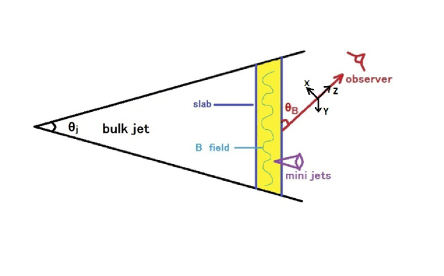
Figure 1: GRB prompt emission and polarization within a compressed slab. Shock propagation is in the bulk jet structure and turbulence occurs behind the shock front. Random and small-scale magnetic field are generated by turbulence in a three-dimensional cube. This cube can be compressed to be a two-dimensional slab. GRB prompt emission is the total emission from those mini-jets. The GRB prompt polarization feature is dependent on the magnetic field configuration. $B_{x}=B_{0}\rm{cos}\phi\rm{sin}\theta_{B}$ and $B_{y}=B_{0}\rm{sin}\phi$ are two components in the slab plane, where $\phi$ is the azimuthal angle at any point randomly distributed in the slab plane (Laing, 1980). The angle between the line of sight from the observer and the slab plane is labeled as $\theta_{B}$.

Magnetic field configurations is a dominant issue for the research of GRB radiation and polarization. In this paper, we apply the topology of random magnetic fields introduced by Laing (1980, 2002). A three-dimensional cube containing random and small-scale magnetic fields can be compressed into a two-dimensional slab by relativistic shocks. In the slab plane, the distribution of magnetic fields is still stochastic. The magnetic field vector at one point, denoted in rectangular coordinates, is ${\bf B}=B_{0}(\cos\phi\sin\theta_{B},\sin\phi,\cos\phi\cos\theta_{B})$, where $\theta_{B}$ is the angle between the slab plane and the line of sight (see Figure 1) and $\phi$ is the azimuthal angle at any point randomly distributed in the slab plane. The position angle of the $E$-vector $\chi$ can be given as $\cos 2\chi=-(\sin^{2}\theta_{B}-\tan^{2}\phi)/(\sin^{2}\theta_{B}+\tan^{2}\phi)$. Thus, the magnetic field acting on the radiation is $B=B_{0}(\cos^{2}\phi\sin^{2}\theta_{B}+\sin^{2}\phi)^{1/2}$. Because an electron obtains same acceleration on average from different directions in a random and small-scale magnetic field, the electron trajectory of jitter radiation can be approximated as a straight line (Medvedev, 2000; Medvedev et al., 2011). Thus, jitter radiation is limited to the small radiation cone along the line of sight to the observer. Since the acceleration term of jitter radiation is proportional to $B^{2}$, we can do a decomposition of jitter radiation in the electron radiation plane and obtain the polarization degree (see the detailed examination in the Appendix). If the slab is orientated so that the $E$-vector of the polarization radiation has a position angle of zero degrees, then the Stokes parameter $U=0$. Following the magnetic field topology given by Laing (1980, 2002), we obtain Stokes parameters of single electron jitter radiation given by: $I=C\int_{0}^{2\pi}(\cos^{2}\phi\sin^{2}\theta_{B}+\sin^{2}\phi)d\phi$, $Q=I\rm{cos}2\chi=-C\int_{0}^{2\pi}(\cos^{2}\phi\sin^{2}\theta_{B}-\sin^{2}\phi)d\phi$, $U=0$, and $V=0$, where $C=C(\gamma,B_{0})$. With a certain electron energy distribution $N(\gamma)$, we obtain the following Stokes parameters of the gross jitter radiation:

$$I=\int^{\gamma_{2}}_{\gamma_{1}}C(\gamma,B_{0})N(\gamma)d\gamma\int_{0}^{2\pi}(\cos^{2}\phi\sin^{2}\theta_{B}+\sin^{2}\phi)d\phi,$$ (5)

$$Q=-\int^{\gamma_{2}}_{\gamma_{1}}C(\gamma,B_{0})N(\gamma)d\gamma\int_{0}^{2\pi}(\cos^{2}\phi\sin^{2}\theta_{B}-\sin^{2}\phi)d\phi,$$ (6)

$$U=0,$$ (7)

and

$$V=0.$$ (8)

Thus, the final polarization degree of the gross jitter emission is

$$\Pi=\frac{Q}{I}=-\frac{\int_{0}^{2\pi}(\cos^{2}\phi\sin^{2}\theta_{B}-\sin^{2}\phi)d\phi}{\int_{0}^{2\pi}(\cos^{2}\phi\sin^{2}\theta_{B}+\sin^{2}\phi)d\phi}.$$ (9)

In our case, we emphasize that the magnetic field configuration is the only parameter that impacts the jitter polarization. Moreover, this polarization result is only valid in the jitter radiation case where the electron deflection angle is small (see Equation (11) in Section 4). Thus, in this two-dimensional case, we only select electrons moving roughly perpendicular to the slab plane.

We present synchrotron polarization of a single electron applying the same magnetic field topology in the Appendix. We also repeat the Stokes parameters of the gross synchrotron radiation given by Laing (1980): $I=C(\gamma,B_{0})\int_{0}^{2\pi}(\cos^{2}\phi\sin^{2}\theta_{B}+\sin^{2}\phi)^{(\nu_{S}+1)/2}d\phi$, $Q=-C(\gamma,B_{0})(\frac{3\nu_{S}+3}{3\nu_{S}+5})\int_{0}^{2\pi}(\cos^{2}\phi\sin^{2}\theta_{B}+\sin^{2}\phi)^{(\nu_{S}-1)/2}(\cos^{2}\phi\sin^{2}\theta_{B}-\sin^{2}\phi)d\phi$, $U=0$, and $V=0$, where $\nu_{S}$ is the synchrotron spectral index. We compare synchrotron polarization and jitter polarization in Figure 2. In this paper, we neglect the effect of light propagation in a thick and highly magnetized plasma screen (Macquart & Melrose, 2000).

2.3 Jet-in-jet Scenario

The mini-jets emit photons in a bulk GRB jet. We simply take into account the geometric effect of the bulk jet. The solid angle element of the jet is $2\pi$sin$\theta$$d\theta$. Since observers always see the forward jet and the backward jet is not observed, the detection probability is half of the result of above the estimation. As the full opening angle is $\theta$, we suggest an upper limit of the integral to be $\theta/2$. The probability should be normalized by the entire solid angle of $4\pi$. Thus, the observational probability of these mini-jets in a bulk GRB jet can be calculated as $P=\pi\int_{0}^{\theta/2}\sin\theta^{\prime}d\theta^{\prime}/4\pi=1/32\Gamma^{2}$ and $\Gamma\sim\theta$. The gross Lorentz factor $\Gamma$ was given by Giannios et al. (2010) as $\Gamma=2\Gamma_{j}\Gamma_{t}/\alpha^{2}$, where $\Gamma_{j}\sim\Gamma_{sh}$ is the Lorentz factor of the bulk jet, $\Gamma_{t}$ is the Lorentz factor of relativistic turbulence in these mini-jets, and textbf$\alpha$ is the “off-axis” parameter defined as $\theta_{j}=\alpha/\Gamma_{j}$. From the investigation of the mini-jets emitting angle distribution (Giannios et al., 2010), the range of $\alpha$ is given as $0<\alpha<2$. We can furthermore estimate the number of mini-jets affected by the turbulent fluid as $n(\gamma)=4\pi R^{2}\Gamma_{j}ct_{\rm{cool}}/l_{s}^{3}$, where $R$ is the fireball radius and $t_{\rm{cool}}=6\pi m_{e}c/\sigma_{T}\gamma B^{2}$ is the cooling timescale of relativistic electrons. The length scale of those mini-jets is $l_{s}=\gamma\Gamma_{t}ct_{\rm{cool}}$. As the number of mini-jets $n(\gamma)$ is a function of the electron Lorentz factor $\gamma$, the electron energy distribution $N_{e}(\gamma)$ is required to obtain a total number of mini-jets given by $n=\int^{\infty}_{1}n(\gamma)N_{e}(\gamma)d\gamma/\int^{\infty}_{1}N_{e}(\gamma)d\gamma$. Due to diffusive shock acceleration, electrons can be accelerated and a power-law energy distribution is given. In our paper, turbulence is considered not only to generate magnetic fields but also to accelerate electrons and the electron energy distribution has a Maxwellian component (Stawarz & Petrosian, 2008). If turbulent acceleration is considered in addition to shock acceleration, the electron energy distribution has a dual-natured shape with a Maxwellian component and a power-law component (Giannios & Spitkovsky, 2009):

$$N_{e}(\gamma)=\left\{\begin{array}[]{l l}C\gamma^{2}\rm{exp}(\gamma/\Theta)/2\Theta^{3},&\gamma\leq\gamma_{th},\\ C\gamma_{th}^{2}\rm{exp}(\gamma_{th}/\Theta)(\gamma/\gamma_{th})^{p_{e}}/2\Theta^{3},&\gamma>\gamma_{th},\\ \end{array}\right.$$ (10)

where $C$ is a constant. In the case that only a fraction of electrons have a non-thermal distribution, we take the characteristic temperature to be $\Theta=kT/m_{e}c^{2}\sim 100$. In our calculation, we adopt $\gamma_{th}=10^{3}$; $p_{e}=2.2$ is the power-law index. Combined with the observational probability $P$ and the total number $n$ of mini-jets affected by turbulence, the final observed polarization degree is $\Pi_{obs}=nP\Pi$.

3 Results

The intrinsic polarization results of GRB prompt emission without jet effects are shown in Figure 2. The jitter polarization degree is strongly dependent on $\theta_{B}$, which is the angle between the line of sight and the slab plane. If the line of sight is perpendicular to the slab plane, we successfully obtain jitter photons, but jitter radiation in the electron radiative plane is symmetric and the polarization degree is zero. Except in this extreme case, the degree of polarization can be measured with different values of $\theta_{B}$. With the same magnetic field configuration, we can compare jitter polarization and synchrotron polarization. Both jitter polarization and synchrotron polarization are related to $\theta_{B}$. On the other hand, as we discussed in Section 2.2, jitter polarization is not related to the radiation spectrum and it can reach a maximum value of 100 percent. Synchrotron polarization (see details in the Appendix) is related to the radiation spectral index and its maximum value is $(\nu_{S}+3)/(\nu_{S}+5)$. The cases of $\nu_{s}=2.0,1.0$, and 0.6 are shown in Figure 2 as examples.

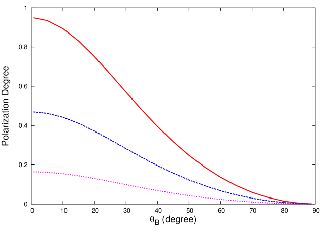
Figure 3: Observational jet “off-axis” effect on GRB prompt polarization. The solid line (red), the long-dashed line (blue), and the short-dashed line (pink) denote the jitter polarization results given by “off-axis” parameter values of 1.55, 1.3, and 1.0, respectively. The shock Lorentz factor $\Gamma_{sh}$ is fixed at 100.

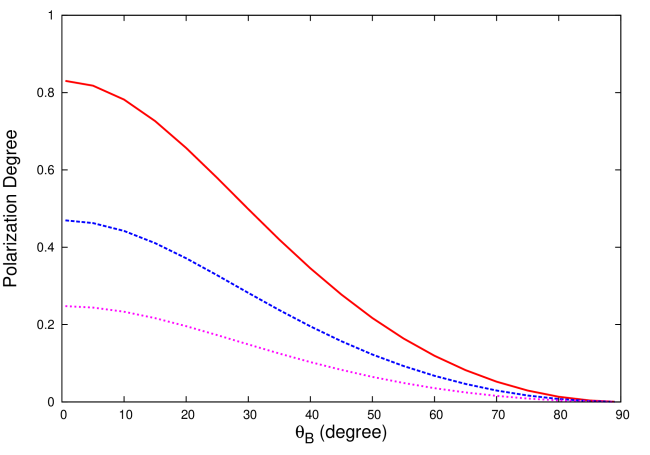
Figure 4: Shock Lorentz factor effect on GRB prompt polarization. The solid line (red), the long-dashed line (blue), and the short-dashed line denote the jitter polarization results given by shock Lorentz factors $\Gamma_{sh}$ of 85, 100, and 120, respectively. The “off-axis” parameter is taken to be 1.3.

We further provide examples of the observed jitter polarization degree in our jet-in-jet scenario shown in Figures 3 and 4. Different jet “off-axis” parameters, 1.55, 1.3 and 1.0, are used to calculate the observed polarization degree shown in Figure 3. Here, we take $\Gamma_{sh}=100$, $\Gamma_{t}=10$, and $R=10^{13}$ cm. We show that the polarization degree is significantly sensitive to the jet “off-axis” parameter. A stronger jet “off-axis” effect yields a stronger observed polarization degree. In Figure 4, we present examples of jitter polarization results affected by the shock Lorentz factor $\Gamma_{sh}$. We fix the “off-axis” parameter as 1.3, $\Gamma_{t}=10$, and $R=10^{13}$ cm. Shock Lorentz factor values of 85, 100, and 120 are adopted. We see that a low polarization degree can be induced by a large shock Lorentz factor. This fact suggest that a large shock Lorentz factor provides powerful radiation along the jet axis while a powerful polarization can be measured in the strong off-axis case, which has a relatively small Lorentz factor and weak radiation.

It is also useful to review the GRB polarization feature under the mechanism of synchrotron radiation in the jet structure. Gruzinov (1999) and Sari (1999) proposed the possibility of high-degree GRB polarization. Granot (2003) comprehensively discussed different GRB jet polarization cases. Here, for simplicity, we apply the model of Gruzinov (1999) to illustrate the configuration differences between the tangled magnetic field and the ordered magnetic field. The polarization degree derived from the magnetic field parallel/perpendicular to the jet direction was given as $\Pi=\Pi_{0}\sin^{2}\alpha_{B}(B^{2}_{\parallel}-0.5B^{2}_{\perp})/[B^{2}_{\parallel}\sin^{2}\alpha_{B}+0.5B^{2}_{\perp}(1+\cos^{2}\alpha_{B})]$, where $B_{\parallel}$ is the magnetic field parallel to the shock propagation direction, $B_{\perp}$ is the magnetic field perpendicular to the shock propagation, and $\alpha_{B}=\pi/2-\theta_{B}$ is the angle between the line of sight from observer and the direction of the shock propagation (Gruzinov, 1999). In our model, we have fully obtained the polarization feature of GRB prompt emission in the case of $B_{\parallel}\ll B_{\perp}$ (Laing, 1980, 2002) and this condition is necessary for jitter radiation. If $B_{\parallel}\gg B_{\perp}$, the polarization degree is $\Pi\sim\Pi_{0}$, which is the result obtained from an ordered magnetic field aligned with the jet direction. This result reproduces exactly the polarization degree of synchrotron radiation as $\Pi_{0}=(3\nu_{S}+3)/(3\nu_{S}+5)$; the electron energy distribution has a power-law distribution with a power-law index $p_{e}$ and $\nu_{S}=(p_{e}-1)/2$. Considering a certain jet structure and line of sight effects, a high degree of GRB prompt polarization can be obtained (Granot, 2003; Lazzati & Begelman, 2009). In our paper, the two-dimensional magnetic slab and the jet-in-jet structure provide the possibility of asymmetric radiation in the electron radiative plane. Thus, the GRB prompt emission can be highly polarized as well.

4 Discussion and Conclusions

Relativistic electrons accelerated by diffusive shock acceleration with a power-law energy distribution can emit high-energy photons in an ordered magnetic field. Therefore, it is possible to explain the high-degree polarization detected in GRB prompt emission by synchrotron radiation. Alternatively, we present in this paper that turbulence can accelerate electrons and generate random and small-scale magnetic fields. The relativistic electrons emit X-ray/$\gamma$-ray jitter photons in the jet-in-jet structure. Some important physical components, such as turbulence behind the shock front, random and small-scale magnetic fields, the electron energy distribution, and mini-jets, are self-consistently organized in the process of jitter radiation. We obtain a high-degree polarization of GRB prompt emission through jitter radiation considering a two-dimensional compressed magnetic field configuration. The intrinsic polarization degree is a function of the angle between the line of sight and the slab plane, and large polarization values can be achieved in the case of small angles. Moreover, the final observed polarization degree in the jet-in-jet scenario is affected by the “off-axis” parameter and the shock Lorentz factor.

In this paper, the electron trajectory of jitter radiation in random and small-scale magnetic fields is assumed to be a straight line. In other words, the condition of $\theta_{d}\ll 1/\gamma$ should be satisfied by jitter radiation (Medvedev et al., 2011). Here, $\theta_{d}=eB\lambda_{B}/\gamma m_{e}c^{2}$ is the deflection angle of electrons in a magnetic field, and $\lambda_{B}\sim c/\omega_{pe}$ is the length scale of the magnetic field. We obtain

$$\theta_{d}=(\frac{B}{1.2\times 10^{6}~{}\rm{G}})(\frac{n}{1.5\times 10^{19}~{}\rm{cm^{-3}}})^{-1/2}(\frac{\Gamma_{sh}}{100})^{1/2}\gamma^{-1}.$$ (11)

This condition is strongly dependent on the magnetic field and the electron number density. We constrain the condition of jitter radiation in an example below. The electron number density is given by $n=N/\Delta\Omega R^{2}\Delta R$. $N=1.0\times 10^{52}\sim 6\times 10^{54}$ is the total number of electrons in the radiative region (Kumar & Narayan, 2009). We take the fireball radius to be $R=10^{13}~{}\rm{cm}$ and fireball shell to be $\Delta R=10^{10}~{}\rm{cm}$. If the jet opening angle is about 5 degree, we obtain a solid angle $\Delta\Omega=3.3\times 10^{-4}$ and the estimated value of number density is $n=3.0\times 10^{20}~{}\rm{cm^{-3}}\sim 1.8\times 10^{22}~{}\rm{cm^{-3}}$. Thus, $\theta_{d}\ll 1/\gamma$ and the electron trajectory can be treated as a straight line. In order to satisfy this jitter condition in the two-dimensional case, we select electrons moving roughly perpendicular to the slab plane so that the electron deflection angle is small. The general case of electrons moving in a random walk in a stochastic magnetic field with a large deflection angle was discussed by Fleishman (2006) and numerical simulations may be required to solve this complicated issue.

It is expected that the so-called depolarization due to the Faraday rotation of the polarization screen (Burn, 1966) can be a powerful tool to further constrain the source structure and magnetic field topology. In general, stochastic Faraday rotation creates a polarization degree of $\Pi\propto\rm{exp}(-\lambda^{4})$, where $\lambda$ is wavelength (Melrose & Macquart, 1998). Tribble (1991) discussed a power-law structure function for a Faraday rotation measurement. The polarization degree was given as $\Pi\propto\lambda^{-4/m}$, where $m$ is related to the turbulent cascade. Even if we consider a polarization fluctuation proportional to $\lambda$, the final polarization degree still dramatically decreases as $\Pi\propto\lambda^{-2.2}$ if we adopt a typical value of $m=\zeta_{p}-2$ given in our model. Therefore, GRB prompt polarization measured in the soft band is about 20% of that measured in the hard band. This prediction can be examined by future observations if GRB prompt polarization measurements can be performed simultaneously in different energy bands. This simple analysis of the depolarization effect also indicates that GRB prompt polarization in optical bands is nearly impossible detect even if GRB is highly polarized in high-energy bands. On the other hand, the polarization of GRB optical afterglows was detected. The radiation case of external shocks of GRBs sweeping into the surrounding interstellar medium is beyond the scope of this paper. Here, we make some simple speculations. As optical afterglow is onset at early times after the GRB is triggered, and the jet is strongly anisotropic with a narrow beaming angle. Thus, the optical polarization degree can reach values of 10% (Uehara et al., 2012) and even higher polarization degrees were expected (Steele et al., 2009). In late times after a GRB is triggered, the beaming angle of the jet is wide and the jet anisotropy is not prominent. Thus, the polarization of the optical afterglow is weak (Covino et al., 1999; Hjorth et al., 1999; Wijers et al., 1999). Moreover, high-energy photons from GRB prompt emission can pass through a dense medium without being strongly absorbed. Thus, the depolarization effect is weak and a high polarization degree can be detected, while UV/optical photons of GRB afterglows can be strongly absorbed by the surrounding dense material. Therefore, even though the initial polarization degree of GRB optical afterglows is very high, the external depolarization effect is strong as the diffraction in a Faraday prism is taken into account (Sazonov, 1969; Macquart & Melrose, 2000). Thus, due to the strong depolarization effect, the detected polarization degree of GRB optical afterglows is low. Further quantitative computations can be executed since the magnetic field configuration adopted in this paper is still valid for the depolarization cases mentioned above (Rossi et al., 2004).

Rapid time variations of the polarization angle and polarization degree have been measured either in GRB prompt emission cases (Götz et al. (2009) for GRB 041219A and Yonetoku et al. (2011) for GRB 100826A) or in GRB afterglow cases (Rol et al. (2000) for GRB 990712, Greiner et al. (2003) for GRB 030329, and Wiersema et al. (2012) for GRB 091018). The observed timescale of polarization variation in GRB prompt emission is about 50-100 s (Yonetoku et al., 2011), which corresponds to an intrinsic timescale of 0.5-1 s. Here, we list three possibilities to explain this rapid variation. First, GRB helical jets with helical magnetic fields and helical rotation generated by black holes (Mizuno et al., 2012) should be considered. With a helical jet, the slab may rotate and the magnetic field configuration may change quickly. Then, rapid polarization variation occurs. Second, Lazzati & Begelman (2009) proposed that faint pulses of GRB prompt emission are a main contributor to the polarization. If this is true, we can obtain the rapid time variation of the polarization since the pulses shown in GRB prompt lightcurves show rapid variation; Third, the turbulent feature in the slab should be revisited. We estimate the variability of GRB prompt polarization due to the variability of stochastic eddies as $\delta t\sim l_{eddy}/c_{s}$. Given $l_{eddy}\sim R/\Gamma_{j}\Gamma_{t}$ and $c_{s}\sim c/\sqrt{3}$, $\delta t$ is about 1.7 s, which can be comparable to the observational timescale. Moreover, small-scale fluid turbulence and magnetic reconnection was suggested by Matthews & Scheuer (1990b). Recently, Zhang & Yan (2011) and McKinney & Uzdensky (2012) illustrated the possibility of magnetic reconnection for GRB energy dissipation. We suggest that small-scale magnetic reconnection in the compressed slab is likely to affect the rapid polarization variation. More observations (TSUBAME, NuSTAR, Astro-H) and quantitative explanations in detail are expected in the future.

Appendix A Polarization of Single Electrons in A Random Magnetic Field

In this Appendix, we first introduce the polarization feature of single relativistic electrons in a magnetic field assuming jitter condition. We repeat the radiation property by Landau & Lifshitz (1971) as

$$E_{\omega}=\frac{1}{2\pi}\int{Ee^{i\omega t}dt},$$ (A1)

where the retarded time is $t^{\prime}=t-R(t^{\prime})/c\cong t-R_{0}/c+{\bf n}\cdot{\bf r}(t^{\prime})/c\cong t-R_{0}/c+{\bf n}\cdot{\bf v}t^{\prime}/c$; ${\bf n}$ is the radiation direction. If we take $dt=dt^{\prime}(1-{\bf n}\cdot{\bf v}/c)$, we obtain

$$E_{\omega}=\frac{e}{c^{2}}\frac{e^{ikR_{0}}}{R_{0}(1-{\bf n}\cdot{\bf v}/c)^{2}}\int{\bf n}\times\{({\bf n}-{\bf v}/c)\times{\bf w}(t^{\prime})\}e^{i\omega t^{\prime}(1-{\bf n}\cdot{\bf v}/c)}dt^{\prime}.$$ (A2)

If we adopt the notation $\omega^{\prime}=\omega(1-{\bf n}\cdot{\bf v}/c)$, we obtain

$$E_{\omega}=\frac{e}{c^{2}}\frac{e^{ikR_{0}}}{R_{0}}(\frac{\omega}{\omega^{\prime}})^{2}{\bf n}\times\{({\bf n}-{\bf v}/c)\times{\bf w}_{\omega^{\prime}}\}.$$ (A3)

The acceleration term is ${\bf w_{\omega^{\prime}}}=e{\bf v}\times{\bf B}/\gamma m_{e}c$. The electron trajectory is necessary to obtain the acceleration term and the calculation in Equation (A3). If the electron trajectory can be treated as a straight line in a magnetic field (see Equation (11) of jitter radiation condition), we have a compressed magnetic slab plane with an angle of $\theta_{B}$ to the radiative $X-Y$ plane, and the electron velocity is perpendicular to the slab plane since the electron deflection angle of the jitter radiation is smaller than $1/\gamma$. The jitter radiation direction follows the direction of the electron. Thus, we obtain the $X$-axis component as

$$E_{x}=\frac{e^{2}B_{y}}{2\gamma^{3}m_{e}c^{2}}(\frac{\omega}{\omega^{\prime}})^{2}\frac{e^{ikR_{0}}}{R_{0}}$$ (A4)

and the $Y$-axis component as

$$E_{y}=-\frac{e^{2}B_{x}}{2\gamma^{3}m_{e}c^{2}}(\frac{\omega}{\omega^{\prime}})^{2}\frac{e^{ikR_{0}}}{R_{0}}.$$ (A5)

The radiation intensity is $I=c|E|^{2}R_{0}^{2}/2\pi$. The Stokes parameters can be defined as

$$I=<E_{x}E^{\ast}_{x}>+<E_{y}E_{y}^{\ast}>=\frac{e^{4}}{8\pi\gamma^{6}m_{e}^{2}c^{3}}(\frac{\omega}{\omega^{\prime}})^{4}(B^{2}_{x}+B_{y}^{2})$$ (A6)

and

$$Q=<E_{x}E^{\ast}_{x}>-<E_{y}E_{y}^{\ast}>=\frac{e^{4}}{8\pi\gamma^{6}m_{e}^{2}c^{3}}(\frac{\omega}{\omega^{\prime}})^{4}(B^{2}_{y}-B_{x}^{2}).$$ (A7)

From Section 2.2, we know $B_{x}=B_{0}\rm{cos}\phi\rm{sin}\theta_{B}$ and $B_{y}=B_{0}\rm{sin}\phi$. Finally, we obtain the jitter polarization $\Pi=Q/I$, which is only related to the configuration of the magnetic field; Equation (9) is verified.

In this Appendix, we also review the synchrotron polarization of a single electron. We keep the same random magnetic field topology used in the jitter polarization case to calculate the synchrotron polarization and we can repeat the calculation of Laing (1980). The radiation intensity of the synchrotron mechanism is

$$I=\frac{2\pi\sqrt{3}e^{2}\nu_{L}}{c}[\frac{\nu}{\nu_{c}}\int^{\infty}_{\nu/\nu_{c}}K_{5/3}(t)dt],$$ (A8)

where $\nu_{c}=(3/2)\gamma^{2}\nu_{L}$, $\nu_{L}=eB/(2\pi m_{e}c)$ is the Larmor frequency ,and $K$ is a modified Bessel function. The synchrotron polarization of a single electron is

$$\Pi=\frac{K_{2/3}(\nu/\nu_{c})}{\int_{\nu/\nu_{c}}^{\infty}K_{5/3}(t)dt},$$ (A9)

related to the magnetic field, electron Lorentz factor $\gamma$ and radiation frequency $\nu$ (Rybicki & Lightman, 1979).

In order to compare synchrotron polarization with jitter polarization, we apply the same magnetic field topology described in Section 2.2 to synchrotron polarization; our results are shown in Figure 5. In the calculation, we fix the magnetic field value at $1.3\times 10^{6}~{}\rm{G}$. For a given $\theta_{B}$, the degree of synchrotron polarization increases, if the radiation is toward a higher frequency $\nu$ and/or the electron Lorentz factor $\gamma$ tends toward smaller values. This property is typical of synchrotron polarization of single electrons. In Figure 5, we plot the jitter polarization as well, which is independent of the radiation frequency $\nu$ and the electron Lorentz factor $\gamma$. Even though synchrotron polarization degrees can be coincidentally the same as the jitter polarization degree by adjusting the parameters of $\nu$ and $\gamma$, we emphasize that jitter polarization and synchrotron polarization are physically different because jitter radiation and synchrotron radiation are two different radiation mechanisms.

If the synchrotron power-law spectrum with a power-law index $\nu_{S}$ is given and an electron energy distribution is assumed to be a power-law with an index of $2\nu_{S}+1$, we obtain the Stokes parameters of the gross electrons:

$$I=C\int_{0}^{2\pi}(\cos^{2}\phi\sin^{2}\theta_{B}+\sin^{2}\phi)^{(\nu_{s}+1)/2}d\phi,$$ (A10)

$$Q=-C\frac{(3\nu_{S}+3)}{(3\nu_{S}+5)}\int_{0}^{2\pi}(\cos^{2}\phi\sin^{2}\theta_{B}+\sin^{2}\phi)^{(\nu_{s}-1)/2}(\cos^{2}\phi\sin^{2}\theta_{B}-\sin^{2}\phi)d\phi,$$ (A11)

$$U=0,$$ (A12)

and

$$V=0,$$ (A13)

where $C$ is constant. Thus, the final polarization degree of the gross synchrotron emission is

$$\Pi=\frac{Q}{I}=-\frac{(3\nu+3)}{(3\nu_{s}+5)}\frac{\int_{0}^{2\pi}(\cos^{2}\phi\sin^{2}\theta_{B}+\sin^{2}\phi)^{(\nu_{s}-1)/2}(\cos^{2}\phi\sin^{2}\theta_{B}-\sin^{2}\phi)d\phi}{\int_{0}^{2\pi}(\cos^{2}\phi\sin^{2}\theta_{B}+\sin^{2}\phi)^{(\nu_{s}+1)/2}d\phi}.$$ (A14)

These are the results given by Laing (1980) and we also plot them in Figure 2.

Figure 2: Intrinsic polarization degree as a function of $\theta_{B}$. The solid line (red) denotes the polarization result of jitter radiation. The long-dashed line (blue), the short-dashed line (pink), and the dotted line (cyan) denote the polarization results calculated from synchrotron radiation with a spectral index of 2.0, 1.0, and 0.6, respectively.

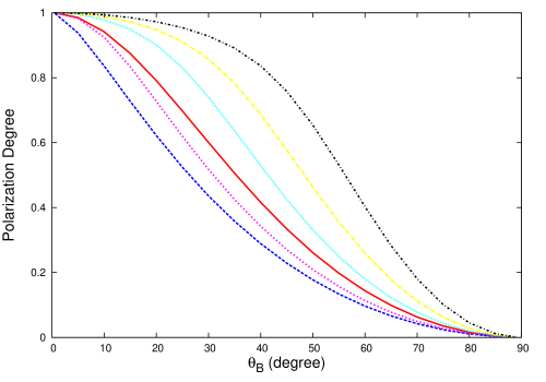
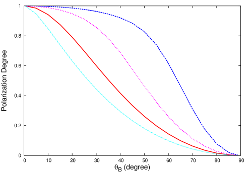
Figure 5: Synchrotron polarization vs jitter polarization for a single electron. Top panel: synchrotron polarization degree results are calculated as a function of $\theta_{B}$ with radiation frequencies of $\nu=1~{}\rm{keV}$, $\nu=50~{}\rm{keV}$, $\nu=250~{}\rm{keV}$, $\nu=500~{}\rm{keV}$, and $\nu=1~{}\rm{MeV}$ denoted by the long-dashed line (blue), the short-dashed line (pink), the dotted line (cyan), the long-dash-dotted line (yellow), and the short-dash-dotted line (black), respectively. The electron Lorentz factor is fixed at $\gamma=10^{3}$. Bottom panel: synchrotron polarization degree results calculated as a function of $\theta_{B}$ with electron Lorentz factors $\gamma=500$, $\gamma=10^{3}$, and $\gamma=10^{4}$ denoted by the long-dashed line (blue), the short-dashed line (pink), and the dotted line (cyan), respectively. The radiation frequency is fixed at $\nu=500~{}\rm{keV}$. The jitter polarization denoted by the solid line (red) is shown in both panels as well.

References

- Bersier et al. (2003) Bersier, D., et al. 2003, ApJ, 583, L63
- Bhatt & Bhattacharyya (2012) Bhatt, N., & Bhattacharyya, S. 2012, MNRAS, 420, 1706
- Burn (1966) Burn, B. J. 1966, MNRAS, 133, 67
- Cawthorne & Cobb (1990) Cawthorne, T. V., & Cobb, W. K. 1990, ApJ, 350, 536
- Coburn & Boggs (2003) Coburn, W., & Boggs, S. E. 2003, Nature, 423, 415
- Covino et al. (1999) Covino, S., et al. 1999, A&A, 341, L1
- Foley (2011) Foley, S. 2011, GCN circ. 11771
- Frederiksen et al. (2010) Frederiksen, J. T., Haugblle, T., Medvedev, M. V., & Nordlund, Å. 2010, ApJ, 722, L114
- Fleishman (2006) Fleishman, G. D. 2006, ApJ, 638, 348
- Ghisellini & Lazzati (1999) Ghisellini, G., & Lazzati, D. 1999, MNRAS, 309, L7
- Giannios & Spitkovsky (2009) Giannios, D., & Spitkosky, A. 2009, MNRAS, 400, 330
- Giannios et al. (2010) Giannios, D., Uzdebsky, D. A., & Begelman, M. C. 2010, MNRAS, 402, 1649
- Götz et al. (2009) Götz, D., Laurent, P., Lebrun, F., Daigne, F., & Bošnjak, Ž. 2009, ApJ, 695, L208
- Granot (2003) Granot, J. 2003, ApJ, 596, L17
- Greiner et al. (2003) Greiner, J., et al. 2003, Nature, 426, 157
- Gruzinov & Waxman (1999) Gruzinov, A., & Waxman, E. 1999, ApJ, 511, 852
- Gruzinov (1999) Gruzinov, A. 1999, ApJ, 525, L29
- Hjorth et al. (1999) Hjorth, J., et al. 1999, Science, 283, 2073
- Hughes et al. (1985) Hughes, P. A., Aller, H. D., & Aller, M. F. 1985, ApJ, 298, 301
- Kalemci et al. (2007) Kalemci, E., Boggs, S, E., Kouveliotou, C., Finger, M., & Baring, M. G. 2007, ApJS, 169, 75
- Kelner et al. (2013) Kelner, S. R., Aharonian, F. A., & Khangulyan, D. 2013, arXiv:1304.0493
- Kumar & Narayan (2009) Kumar, P., & Narayan, R. 2009, MNRAS, 395, 472
- Laing (1980) Laing, R. A. 1980, MNRAS, 193, 439
- Laing (2002) Laing, R. A. 2002, MNRAS, 329, 417
- Landau & Lifshitz (1971) Landau, L. D., & Lifshitz, E. M. 1971, The Classical Theory of Fields (Oxford: Pergamon)
- Lazar et al. (2009) Lazar, A., Nakar, E., & Piran, T. 2009, ApJ, 695, L10
- Lazzati & Begelman (2009) Lazzati, D., & Begelman, M. C. 2009, ApJ, 700, L141
- Lemoine (2013) Lemoine, M. 2013, MNRAS, 428, 845
- Lyutikov (2006) Lyutikov, M. 2006, MNRAS, 369, L5
- Macquart & Melrose (2000) Macquart, J.-P., & Melrose, D. B. 2000, ApJ, 545, 798
- Mao & Wang (2011) Mao, J., & Wang, J. 2011, ApJ, 731, 26
- Mao & Wang (2012) Mao, J., & Wang, J. 2012, ApJ, 748, 135
- Martins et al. (2009) Martins, J. L., Martins, S. F., Fonseca, R. A., & Silva, L. O. 2009, Proc. of SPIE, 7359, 73590V-1-8
- Matthews & Scheuer (1990a) Matthews, A. P., & Scheuer, P. A. G. 1990a, MNRAS, 242, 616
- Matthews & Scheuer (1990b) Matthews, A. P., & Scheuer, P. A. G. 1990b, MNRAS, 242, 623
- McGlynn et al. (2007) McGlynn, S. et al., 2007, A&A, 466, 895
- McKinney & Uzdensky (2012) MvKinney, J. C., & Uzdensky, D. A. 2012, MNRAS, 419, 573
- Medvedev & Loeb (1999) Medvedev, M. V., & Loeb, A. 1999, ApJ, 526, 697
- Medvedev (2000) Medvedev, M. V. 2000, ApJ, 540, 704
- Medvedev (2006) Medvedev, M. V. 2006, ApJ, 637, 869
- Medvedev et al. (2011) Medvedev, M. V., Frederiksen, J. T., Haugblle, T., Nordlund, Å. 2011, ApJ, 737, 55
- Melrose & Macquart (1998) Melrose, D. B., & Macquart, J.-P. 1998, ApJ, 505, 921
- Mészáros et al. (1993) Mészáros, P., Laguna, P., & Rees, M. J. 1993, ApJ, 415, 181
- Mészáros et al. (1994) Mészáros, P., Rees, M. J., & Papathanassiou, H. 1994, ApJ, 432, 181
- Milosavljević et al. (2006) Milosavljević , M., Nakar, E., & Spitkovsky, A. 2006, ApJ, 637, 765
- Mizuno et al. (2012) Mizuno, Y., Lyubarsky, Y., Nishikawa, K.-I., & Hardee, P. E. 2012, ApJ, 757, 16
- Nalewajko (2009) Nalewajko, K. 2009, MNRAS, 395, 524
- Narayan & Kumar (2009) Narayan, R., & Kumar, P. 2009, MNRAS, 394, L117
- Nishikawa et al. (2011) Nishikawa, K.-I., et al. 2011, AdSpR, 47, 1434
- Norris et al. (2005) Norris, J. P., Bonnell, J. T., Kazanas, D., Scargle, J. D., Hakkila, J., & Giblin, T. W. 2005, ApJ, 627, 324
- Piran (2005) Piran, T. 2005, in AIP Conf. Ser. 784, Magnetic Fields in the Universe: From Laboratory and Stars to Primordial Structures, ed. E. M. de Gouveia Dal Pino, G. Lugones, & A. Lazarian (Melville, NY: AIP), 164
- Reynolds et al. (2010) Reynolds, S., Pothapragada, S., & Medvedev, M. V. 2010, ApJ, 713, 764
- Retnolds & Medvedev (2012) Reynolds, S., & Medvedev, M. V. 2012, Physics of Plasmas, 19, 023106
- Rol et al. (2000) Rol, E., et al. 2000, ApJ, 544, 707
- Rossi et al. (2004) Rossi, E. M., Lazzati, D., Salmonson, J. D., & Ghisellini, G. 2004, MNRAS, 354, 86
- Rybicki & Lightman (1979) Rybicki, G., & Lightman, A. P., 1979, Radiative Processes in Astrophysics., Wiely Interscience, New York
- Sari (1999) Sari, R. 1999, ApJ, 524, L43
- Sazonov (1969) Sazonov, V. N. 1969, Soviet Astron., 13, 396
- Schekochihin & Cowley (2007) Schekochihin, A. A., & Cowley, S. T. 2007, in Magnetohydrodynamics: Historical Evolution and Trends, ed. S. Molokov, R. Moreau, & H. K. Moffatt (Berlin: Springer), 85
- Schekochihin et al. (2004) Schekochihin, A. A., Cowley, S. C., Tayler, S. F., Marson, J. A., & McWilliams, J. C. 2004, ApJ, 612, 276
- She & Leveque (1994) She, Z.-S., & Leveque, E. 1994, Phys. Rev. Lett., 72, 336
- She & Waymire (1995) She, Z.-S., & Waymire, E. C. 1995, Phys. Rev. Lett., 74, 262
- Sironi & Spitkovsky (2009) Sironi, L., & Spitkovsky, A., 2009, ApJ, 707, L92
- Stawarz & Petrosian (2008) Stawarz, L., & Petrosian, V. 2008, ApJ, 681, 1725
- Steele et al. (2009) Steele, I. A., Mundell, C. G., Smith, R. J., Kobayashi, S., & Guidorzi, C. 2009, Nature, 462, 767
- Teraki & Takahara (2011) Teraki, Y., & Takahara, F. 2011, ApJ, 735, L44
- Tierney & von Kienlin (2011) Tierney, D., & von Kienlin A. 2011, GCN circ. 12187
- Toma et al. (2009) Toma, K., et al. 2009, ApJ, 698, 1042
- Tribble (1991) Tribble, P. C. 1991, MNRAS, 250, 726
- Uehara et al. (2012) Uehara, T., et al. 2012, ApJ, 752, L6
- Waxman (2003) Waxman, E. 2003, Nature, 423, 388
- Wiersema et al. (2012) Wiersema, K., et al. 2012, MNRAS, 426, 2
- Wijers et al. (1999) Wijers, R. A. M., et al. 1999, apj, 523, L33
- Yonetoku et al. (2011) Yonetoku, D., et al. 2011, ApJ, 743, L30
- Yonetoku et al. (2012) Yonetoku, D., et al. 2012, ApJ, 758, L1
- Zhang & Yan (2011) Zhang, B., Yan, H. 2011, ApJ, 726, 90
- Zrake & MacFadyen (2012) Zrake, J., & MacFadyen, A. I. 2012, arXiv:1210.4066