Current hot spot in the spin-valley blockade in carbon nanotubes

Abstract

We present a theoretical study of the spin-valley blockade transport effect in a double quantum dot defined in a straight carbon nanotube. We find that intervalley scattering due to short-range impurities completely lifts the spin-valley blockade and induces a large leakage current in a certain confined range of the external magnetic field vector. This current hot spot emerges due to different effective magnetic fields acting on the spin-valley qubit states of the two quantum dots. Our predictions are compared to a recent measurement [F. Pei et al., Nat. Nanotech. 7, 630 (2012)]. We discuss the implications for blockade-based schemes for qubit initialization/readout, and motion sensing of nanotube-based mechanical resonators.

I Introduction

Breakthrough experiments in the past decade have demonstrated the ability to initialize, manipulate, couple and read out spin-based quantum bitsLoss and DiVincenzo (1998) (qubits) using electrons in electrostatically defined quantum dots (QDs)Elzerman et al. (2004); Petta et al. (2005); Koppens et al. (2006); Nowack et al. (2007); Hanson et al. (2007). A key ingredient in many of those experiments is the Pauli blockade mechanismOno et al. (2002). Pauli blockade is a characteristic feature of electronic transport through a double quantum dot (DQD) via the (1,1)$\to$(0,2)$\to$(0,1)$\to$(1,1) cycle of charge configurations, where ($n$,$m$) stands for states with $n$ electrons in the first QD and $m$ electrons in the second QD. If a spin-triplet state is occupied in the (1,1) charge configuration, then Pauli’s exclusion principle prevents the (1,1)$\to$(0,2) tunneling process and thereby blocks the current flow. This simple mechanism allows for initialization and readout of spin states via current or charge sensing measurements in a serially coupled double quantum dot (DQD). Pauli blockade measurements have also been utilized to experimentally identify the strengths of spin-orbit and hyperfine interactions in DQDsKoppens et al. (2005); Nadj-Perge et al. (2010). By combining a DQD with a mechanical resonator, the Pauli blockade mechanism can be exploited to convert the fast motional oscillations ($\sim 100$ MHz) of the resonator to a direct current through the DQD, enabling a simple dc electronic detection of the resonator’s motionOhm et al. (2012).

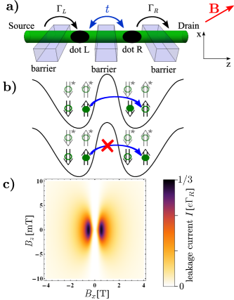
Figure 1: (Color online) (a) Schematic of the carbon nanotube double quantum dot transport setup showing spin-valley blockade. The red arrow represents the external magnetic field $\text{\boldmath{$B$}}=(B_{x},0,B_{z})$. Lead-dot tunneling rates $\Gamma_{L}$, $\Gamma_{R}$ and the coherent interdot tunneling amplitude $t$ are indicated. (b) Schematic of the energy levels involved in the transport cycle $(1,1)\to(0,2)\to(0,1)$. If two electrons form a triplet in the (1,1) charge configuration, then current becomes blocked due to Pauli’s exclusion principle. (c) Current hot spots at finite transverse magnetic field, formed due to the complete lifting of the spin-valley blockade by short-range disorder.

Among the numerous host materials for quantum dots, carbon nanotubes (CNTs) are unique because of the simultaneous presence of the valley degree of freedom of their electrons and the strong spin-orbit interactionKuemmeth et al. (2008); Jespersen et al. (2011a); Steele et al. (2013). The two-valued valley degree of freedom is related to the clockwise or anti-clockwise circulating motion of the electron along the CNT circumference, and is responsible for nominally fourfold degenerate (spin and valley) orbital energy levels in electrostatically defined QDs (see Fig. 1a and b). The two valley states are typically denoted by $K$ and $K^{\prime}$. The main effect of the strong spin-orbit interaction is that it induces a large energy splitting $\Delta_{\rm so}\sim 0.1-3$ meV within each fourfold degenerate orbital QD level. At zero magnetic field the low-energy doublet, depicted as $\Uparrow$ and $\Downarrow$ in Fig. 1b, is formed by a time-reversed pair of states. In the absence of valley mixing, $\Uparrow$ is an up-spin state circulating in one direction along the CNT circumference, and $\Downarrow$ is a down-spin state circulating in the other direction.

It is natural to think of the low-energy doublet $\Uparrow,\Downarrow$ as a spin-valley qubitFlensberg and Marcus (2010); Laird et al. (2013). A resonant manipulation scheme for this qubit in a bent CNT has been proposedFlensberg and Marcus (2010) and experimentally implementedLaird et al. (2013) recently. Here again, the Pauli blockade mechanism, named spin-valley blockadePei et al. (2012); Laird et al. (2013); Pályi and Burkard (2009, 2010) in this context, was used for qubit initialization and readout.

Motivated by recent measurements in CNT DQDsBuitelaar et al. (2008); Churchill et al. (2009a, b); Chorley et al. (2011); Pei et al. (2012); Laird et al. (2013), and the potential experimental applications, here we theoretically describe the spin-valley blockade transport effect in a straight nanotube. The schematic view of such a CNT DQD device and the blocking mechanism are shown in Fig. 1a and b, respectively. Our quantity of interest is the direct current $I$, also known as the leakage current, that flows from the source to the drain through the DQD that is tuned to the spin-valley blockade regime. We calculate the current $I$ as a function of the magnitude and direction of the external magnetic field $B$. In our model we include spin-orbit interaction and short-range disorder, allow for both longitudinal and transverse vector components of the magnetic field with respect to the CNT axis, and use the two-site Hubbard model to describe interdot tunneling and the Coulomb repulsion between electrons on the DQD. We focus on the case of clean devices, defined by the condition that the characteristic energy scale of short-range disorder is exceeded by that of the spin-orbit interaction.

Our main result is that for a generic distribution of short-range impurities, a current hot spot, i.e., a region of high current, appears if the magnetic field vector is approximately transverse to the CNT axis, and its magnitude is tuned within a certain range. An example is shown in Fig. 1c, where the current hot spots are located in the vicinity of $|B_{x}|\approx 0.5$ T. The current hot spot emerges because the spin-valley blockade is completely lifted due to the interplay of the short-range impurities and the appropriately tuned transversal magnetic field. Below we show that the transverse magnetic field corresponding to the center of the hot spot is proportional to the energy scales of spin-orbit coupling $\Delta_{\rm so}$ and interdot tunneling $t$, and inversely proportional to the energy scale $\Delta_{KK^{\prime}}$ of short-range disorder [see Eq. (22)]. The current hot spot is most pronounced for zero energy detuning $\epsilon=0$ between the (1,1) and (0,2) states, and gradually disappears as the magnitude of detuning is increased above the energy scale of the interdot tunneling. By utilizing the pseudospin-1/2 description of the spin-valley qubit introduced by Flensberg and MarcusFlensberg and Marcus (2010), and the master-equation model of Pauli blockade in spinful DQDs developed in Refs.  Jouravlev and Nazarov, 2006 and   Coish and Qassemi, 2011, we describe the blockade-lifting mechanism both on a quantitative and a qualitative level. The mechanism found here is relevant for applications relying on the Pauli blockade effect such as qubit initialization/readoutLaird et al. (2013) and the dc electronic motion sensing of a CNT mechanical resonatorOhm et al. (2012) via the qubit-phonon couplingRudner and Rashba (2010); Pályi et al. (2012).

We note that our present work extends Ref. Pályi and Burkard, 2010 where the leakage current was calculated in a longitudinal magnetic field. A number of further theoretical works studied distinct characteristics of Pauli blockade in CNTs, including descriptions of the pulsed-gated DQD experiments of Ref. Churchill et al., 2009aReynoso and Flensberg (2011, 2012), the spectrum of two-electron singleWunsch (2009); Secchi and Rontani (2009) and doubleWeiss et al. (2010) QDs, and the leakage current influenced by the formation of an electronic Wigner moleculevon Stecher et al. (2010) and by hyperfine interactionPályi and Burkard (2009); Kiss et al. (2011).

The rest of the paper is organized as follows. In Sec. II, we reformulate the pseudospin-1/2 descriptionFlensberg and Marcus (2010) of the single-electron spin-valley qubit in a single CNT QD. In Sec. III we revisit the master-equation modelJouravlev and Nazarov (2006); Coish and Qassemi (2011) of the Pauli blockade, and derive our central analytical formula for the leakage current. In Sec. IV we present and interpret our results, which is followed by a discussion in Sec. V.

II Effective magnetic field felt by the spin-valley qubit

Here we consider a single QD with a single electron occupying the nominally fourfold degenerate (spin and valley) ground state of an electrostatically defined CNT QD. Following Ref.  Flensberg and Marcus, 2010, we derive the effective magnetic field acting on the spin-valley qubit formed by the lower-lying time-reversed pair of the four states. The effective magnetic field arises as a combined effect of the external magnetic field and disorder-induced valley mixing. The transport theory yielding the leakage current will be based on the concept of the effective magnetic field in the subsequent Section.

The relative orientation of the CNT and the reference frame is shown in Fig. 1a. The $4\times 4$ Hamiltonian describing the effects of spin-orbit interaction, valley mixing, and external magnetic field on a single spin-valley-degenerate QD level is $H=H_{0}+H_{1}$, where

$$H_{0}=-\frac{\Delta_{\rm so}}{2}\tau_{3}s_{z}$$ (1)

and

$$H_{1} = \frac{1}{2}\mathrm{Re}\left(\Delta_{KK^{\prime}}\right)\tau_{1}+\frac{1}{2}\mathrm{Im}\left(\Delta_{KK^{\prime}}\right)\tau_{2}$$ (2)

$$+ \frac{1}{2}g_{s}\mu_{B}\text{\boldmath{$B$}}\cdot\text{\boldmath{$s$}}+\frac{1}{2}g_{v}\mu_{B}B_{z}\tau_{3}.$$

Here $\Delta_{KK^{\prime}}=|\Delta_{KK^{\prime}}|e^{i\varphi}$ is the complex valley-mixing matrix elementPályi and Burkard (2010, 2011) e.g., induced by short-range disorder, $\tau_{1}$, $\tau_{2}$ and $\tau_{3}$ ($s_{x}$, $s_{y}$ and $s_{z}$) are Pauli matrices acting in valley (spin) space, $g_{s}\approx 2$ is the spin g-factor, $\mu_{B}$ is the Bohr-magneton, and $\text{\boldmath{$B$}}=(B_{x},0,B_{z})$ is the external magnetic field. Finally, $g_{v}$ is the valley g-factor, whose value depends on the chirality of the CNT and ranges approximately between 10 and 50 in experiments using clean CNT QDs Minot et al. (2004); Kuemmeth et al. (2008); Churchill et al. (2009a); Jespersen et al. (2011b); Pei et al. (2012); Steele et al. (2013).

Throughout this work we focus on the spin-orbit-dominated regime of energy scales, i.e.,

$$\Delta_{\rm so}\gg\Delta_{KK^{\prime}},\ g_{v}\mu_{B}B_{z},\ g_{s}\mu_{B}B_{x}.$$ (3)

(Comparisons of order-of-magnitudes, such as Eq. (3), correspond to the absolute values of the involved quantities.) This regime was achieved in recent experiments using relatively clean CNTsKuemmeth et al. (2008); Churchill et al. (2009a, b); Pei et al. (2012); Laird et al. (2013) showing weak valley mixing. Assuming Eq. (3), we treat $H_{1}$ perturbatively. The two-dimensional ground-state (excited-state) subspace of $H_{0}$ is formed by the time-reversed pair $|K\uparrow\rangle$ and $|K^{\prime}\downarrow\rangle$ ($|K\downarrow\rangle$ and $|K^{\prime}\uparrow\rangle$), with energy eigenvalue $-\Delta_{\rm so}/2$ ($\Delta_{\rm so}/2$). In general, valley-mixing and the external magnetic field couples the ground-state and excited-state subspaces. Due to Eq. (3), the coupling between the ground-state and excited-state subspaces can be eliminated by an appropriately chosen (Schrieffer-Wolff) unitary transformationWinkler (2003) of the four-dimensional Hilbert space. This transformation results a $2\times 2$ effective Hamiltonian $H_{\rm eff}$ describing the dynamics within the perturbed ground-state subspace, allowing to describe the electron in that subspace as a spin-1/2 particle in an effective magnetic (Zeeman) field.

The effective Hamiltonian of the ground-state subspace is obtained via the second-order Schrieffer-Wolff transformationWinkler (2003) $U_{\rm SW}=e^{-S}$ , with

$$S=\frac{1}{2\Delta_{SO}}\left[\begin{matrix}0&0&-g_{s}\mu_{B}B_{x}&-\Delta_{KK^{\prime}}\\ 0&0&-\Delta_{KK^{\prime}}^{*}&-g_{s}\mu_{B}B_{x}\\ g_{s}\mu_{B}B_{x}&\Delta_{KK^{\prime}}&0&0\\ \Delta_{KK^{\prime}}^{*}&g_{s}\mu_{B}B_{x}&0&0\end{matrix}\right],$$ (4)

where the basis $\left(|K^{\prime}\uparrow\rangle,|K\downarrow\rangle,|K^{\prime}\downarrow\rangle,|K\uparrow\rangle\right)$ is used. This transformation approximately decouples the ground-state and excited-state subspaces, resulting in the following effective Hamiltonian for the ground-state subspace:

$$H_{\rm eff}=\mathcal{B}_{1}\sigma_{1}+\mathcal{B}_{2}\sigma_{2}+\mathcal{B}_{3}\sigma_{3}\equiv\text{\boldmath{$\mathcal{B}$}}\cdot\text{\boldmath{$\sigma$}},$$ (5)

where

$$\mathcal{B}_{1} = \frac{g_{s}\mu_{B}B_{x}|\Delta_{KK^{\prime}}|\cos\varphi}{2\Delta_{\rm so}},$$ (6a)

$$\mathcal{B}_{2} = \frac{g_{s}\mu_{B}B_{x}|\Delta_{KK^{\prime}}|\sin\varphi}{2\Delta_{\rm so}},$$ (6b)

$$\mathcal{B}_{3} = \frac{1}{2}\left(g_{v}+g_{s}\right)\mu_{B}B_{z},$$ (6c)

and $\sigma_{i}$ is the $i$-th Pauli matrix acting in the perturbed two-dimensional subspace spanned by

$$|\Uparrow\rangle = |K\uparrow\rangle-\frac{g_{s}\mu_{B}B_{x}}{2\Delta_{\rm so}}|K\downarrow\rangle+\frac{\Delta_{KK^{\prime}}}{2\Delta_{\rm so}}|K^{\prime}\uparrow\rangle,$$ (7a)

$$|\Downarrow\rangle = |K^{\prime}\downarrow\rangle+\frac{\Delta_{KK^{\prime}}^{*}}{2\Delta_{\rm so}}|K\downarrow\rangle-\frac{g_{s}\mu_{B}B_{x}}{2\Delta_{\rm so}}|K^{\prime}\uparrow\rangle.$$ (7b)

Furthermore, $\text{\boldmath{$\sigma$}}=(\sigma_{1},\sigma_{2},\sigma_{3})$, and $\text{\boldmath{$\mathcal{B}$}}=(\mathcal{B}_{1},\mathcal{B}_{2},\mathcal{B}_{3})$.

Naturally, the effective Hamiltonian $H_{\rm eff}$ in Eq. (5) takes the form of a Zeeman Hamiltonian describing a spin-1/2 particle in a magnetic field. Accordingly, we will refer to the two basis states of Eq. (7) as representing a pseudospin. For brevity, the effective magnetic field $\mathcal{B}$ is defined in energy units. Note that the first two components of the effective magnetic field $\mathcal{B}$ are nonzero only if both the valley mixing and the transverse magnetic field are nonzero. Furthermore, because of the perturbative character of the first two components of $\mathcal{B}$, the effective Hamiltonian is dominated by $\mathcal{B}_{3}$ unless the external B-field is directed almost perfectly or perfectly along the transversal-to-CNT direction.

In contrast to Ref.   Flensberg and Marcus, 2010, here we kept track of the phase $\varphi$ of the complex valley-mixing matrix element $\Delta_{KK^{\prime}}$, which influences the first two components of the effective magnetic field $\mathcal{B}$. This phase $\varphi$ has no physical significance in a single QD, since its value changes upon multiplying one of the low-energy basis states with an arbitrary complex phase factor. Nevertheless, the difference of the $\varphi$ phases in two QDs $L$ and $R$, i.e., $\Delta\varphi=\varphi_{L}-\varphi_{R}$, does have physical significance. For example, this phase difference influences the leakage current in spin-valley blockade, as shown in Fig. 2. (For further examples, see, eg, Refs. Pályi and Burkard, 2010, 2011; Reynoso and Flensberg, 2012; Culcer et al., 2012; Wu and Culcer, 2012)

III Leakage current in spin-valley blockade

In this Section, we rely on the notion of effective magnetic field $\mathcal{B}$ to calculate the leakage current through a CNT DQD under spin-valley blockade. To this end, we specify the transport problem, and utilize the model introduced in Ref.  Jouravlev and Nazarov, 2006, and the classical master equation outlined in Ref.  Coish and Qassemi, 2011, to derive an analytical result for the leakage current. Conlusions are drawn, and comparison is made to experimental data, in Section IV.

Importantly, we consider the case when only the lower-lying time-reversed pairs of each dot of the DQD participate in transport, i.e., the states $\Uparrow^{*}$ and $\Downarrow^{*}$ in Fig. 1b are disregarded. This case is realized if the source-drain bias voltage and the DQD energy levels are tuned appropriately. In this case, there are 7 states that participate in transport, in complete analogy to spin blockade in GaAsJouravlev and Nazarov (2006). Two of them are single-electron states in the (0,1) charge configuration: $|0,\Uparrow\rangle$ and $|0,\Downarrow\rangle$. Four of them are (1,1) states and there is a single (0,2) state $|S_{g}\rangle\equiv|0,\Uparrow\Downarrow\rangle$, adding up to 5 two-electron states in total. For the (1,1) states, we will use both the product basis $|\Uparrow,\Uparrow\rangle$, $|\Uparrow,\Downarrow\rangle$, $|\Downarrow,\Uparrow\rangle$, $|\Downarrow,\Downarrow\rangle$, and the singlet-triplet basis

$$|S\rangle = \frac{1}{\sqrt{2}}\left(|\Uparrow,\Downarrow\rangle-|\Downarrow,\Uparrow\rangle\right),$$ (8)

$$|T_{0}\rangle = \frac{1}{\sqrt{2}}\left(|\Uparrow,\Downarrow\rangle+|\Downarrow,\Uparrow\rangle\right),$$ (9)

$$|T_{+}\rangle = |\Uparrow,\Uparrow\rangle,$$ (10)

$$|T_{-}\rangle = |\Downarrow,\Downarrow\rangle.$$ (11)

The Hamiltonian describing the DQD is

$$H_{\rm DQD}=H_{t}+H_{\mathcal{B}}+H_{\epsilon}.$$ (12)

Here, $H_{t}$ represents tunneling between the two QDs. We assume spin- and valley-conserving tunneling, which is represented by $H_{t}=\sqrt{2}t(|S_{g}\rangle\langle S|+|S\rangle\langle S_{g}|)$, with $t$ being the tunnel amplitude. Strictly speaking, the spin- and valley-conserving property does not imply the conservation of the pseudospin. Nevertheless, the pseudospin-flip interdot tunneling amplitude is much smaller than $t$, hence we disregard it. The effective magnetic fields, induced by short-range disorder and the external magnetic field, are incorporated in the second Hamiltonian term

$$H_{\mathcal{B}}=\text{\boldmath{$\mathcal{B}$}}_{L}\cdot\text{\boldmath{$\sigma_{L}$}}+\text{\boldmath{$\mathcal{B}$}}_{R}\cdot\text{\boldmath{$\sigma_{R}$}}.$$ (13)

Recall that the short-range disorder configuration on dot $L$ is independent of that on dot $R$, and therefore the disorder-related components [see Eq. (6)] of $\text{\boldmath{$\mathcal{B}$}}_{L}$ are independent of those of $\text{\boldmath{$\mathcal{B}$}}_{R}$. The term $H_{\epsilon}=\epsilon|S_{g}\rangle\langle S_{g}|$ represents the gate-controlled energy detuning between the (1,1) and (0,2) charge configurations. We focus on the zero-detuning case $\epsilon=0$ in this Section, and discuss the case $\epsilon\neq 0$ in Sec. IV.

Once the eigenstates of $H_{\rm DQD}$ are known, the dynamics of current flow can be described by the classical master equationCoish and Qassemi (2011)

$$\dot{p}_{\alpha} = -\left(\sum_{j}W_{j\leftarrow\alpha}\right)p_{\alpha}+\sum_{j}W_{\alpha\leftarrow j}p_{j},$$ (14a)

$$\dot{p}_{j} = -\left(\sum_{\alpha}W_{\alpha\leftarrow j}\right)p_{j}+\sum_{\alpha}W_{j\leftarrow\alpha}p_{\alpha}.$$ (14b)

Here, index $\alpha\in\{1,2,\dots,5\}$ (index $j\in\{1,2\}$) represents two-electron (single-electron) eigenstates of $H_{\rm DQD}$, $p_{\alpha/j}$ are occupation probabilities summing up to unity, i.e., $\sum_{\alpha=1}^{5}p_{\alpha}+\sum_{j=1,2}p_{j}=1$, and $W_{\alpha\leftarrow j}$ ($W_{j\leftarrow\alpha}$) are transition rates representing electron tunneling to the DQD from the left contact (from the DQD to the right contact).

The transition rates are expressed from Fermi’s Golden Rule as

$$W_{\alpha\leftarrow j} = \Gamma_{L}\sum_{\sigma=\Uparrow,\Downarrow}\left|\langle\alpha|d^{\dagger}_{L\sigma}|j\rangle\right|^{2},$$ (15a)

$$W_{j\leftarrow\alpha} = \Gamma_{R}\sum_{\sigma=\Uparrow,\Downarrow}\left|\langle j|d_{R\sigma}|\alpha\rangle\right|^{2},$$ (15b)

where, e.g., $d_{L\Uparrow}$ is an electron operator creating an electron on dot $L$ with pseudospin $\Uparrow$. The rate $\Gamma_{L}$ ($\Gamma_{R}$) is the single-electron tunneling rate at the left (right) contact. The leakage current in the steady state is given by

$$I=\sum_{\alpha j}W_{\alpha\leftarrow j}\bar{p}_{j},$$ (16)

where $\bar{p}_{j}$ is the steady-state occupation probability of the single-electron state $j$.

We are able to analytically diagonalize $H_{\rm DQD}$, and therefore to obtain an analytical formula for the leakage current. The result is expressed with the symmetric and antisymmetric combinations of the effective magnetic fields,

$$\text{\boldmath{$\mathcal{B}$}}_{s}=\frac{1}{2}\left(\text{\boldmath{$\mathcal{B}$}}_{L}+\text{\boldmath{$\mathcal{B}$}}_{R}\right)$$ (17)

and

$$\text{\boldmath{$\mathcal{B}$}}_{a}=\frac{1}{2}\left(\text{\boldmath{$\mathcal{B}$}}_{L}-\text{\boldmath{$\mathcal{B}$}}_{R}\right),$$ (18)

respectively. The resulting formula for the leakage current is

$$\frac{I}{e\Gamma_{R}} = \left[\frac{t^{2}}{4\mathcal{B}_{a}^{\|2}}+\frac{F(\mathcal{B}_{s},\text{\boldmath{$\mathcal{B}$}}_{a})}{4t^{2}\mathcal{B}_{a}^{\perp 2}}-\frac{1}{2}+\frac{\Gamma_{R}}{2\Gamma_{L}},\right]^{-1}$$ (19a)

$$F(\mathcal{B}_{s},\text{\boldmath{$\mathcal{B}$}}_{a}) = (\mathcal{B}_{s}^{2}+\mathcal{B}_{a}^{2}+2t^{2})^{2}-4\mathcal{B}_{s}^{2}(2t^{2}+\mathcal{B}_{a}^{\parallel 2}).$$ (19b)

Here, the vector $\text{\boldmath{$\mathcal{B}$}}_{a}^{\parallel}$ (the vector $\text{\boldmath{$\mathcal{B}$}}_{a}^{\perp}$) is the projection of $\text{\boldmath{$\mathcal{B}$}}_{a}$ onto the direction of $\text{\boldmath{$\mathcal{B}$}}_{s}$, (orthogonal to $\text{\boldmath{$\mathcal{B}$}}_{s}$).

Note that our analytical result (19) is valid irrespective of the energy scale hierarchy between $\mathcal{B}_{a}$, $\mathcal{B}_{s}$ and $t$. In this sense, Eq. (19) interpolates between the zero-detuning limits of the perturbative results Eq. (6) of Ref. Jouravlev and Nazarov, 2006 and Eq. (8) of Ref. Jouravlev and Nazarov, 2006, the former (latter) being valid if $\mathcal{B}_{a}\ll t,\mathcal{B}_{s}$, ($\mathcal{B}_{a},\mathcal{B}_{s}\gg t$). Equation (19) also incorporates the dependence of the leakage current on the tunneling rate $\Gamma_{L}$ at the left lead-dot barrier. In the special case $\Gamma_{L}\gtrsim\Gamma_{R}$ and $B_{a}\ll t,B_{s}$, our Eq. (19) simplifies to

$$\frac{I}{e\Gamma_{R}}=\left[\frac{t^{2}}{4\mathcal{B}_{a}^{\parallel 2}}+\frac{\left(\mathcal{B}_{s}^{2}-2t^{2}\right)^{2}}{4t^{2}\mathcal{B}_{a}^{\perp 2}}\right]^{-1}.$$ (20)

Note that this formula is not identical to Eq. (6) of Ref. Jouravlev and Nazarov, 2006. Difference in the magnitudes of constant factors probably arise from the different definitions of the parameters of the Hamiltonian. In addition, a physically relevant difference is the minus sign in Eq. (20), which substitutes a corresponding plus sign of Eq. (6) of Ref. Jouravlev and Nazarov, 2006. Equation (20) suggests a resonant enhancement of the leakage current at $|\mathcal{B}_{s}|=\sqrt{2}t$. Such an enhancement is indeed expected, since in this case the triplet states polarized parallel or antiparallel to $\text{\boldmath{$\mathcal{B}$}}_{s}$ match the (1,1)-(0,2) hybrid singlet states in energy. Hence we think that the minus sign in Eq. (20) is correct. For the weak-tunneling case $\mathcal{B}_{a},\mathcal{B}_{s}\gg t$, Eq. (19) implies

$$\frac{I}{e\Gamma_{R}}=\frac{t^{2}}{\mathcal{B}_{s}^{2}}\left(\text{\boldmath{$n$}}_{L}\times\text{\boldmath{$n$}}_{R}\right)^{2},$$ (21)

where the vectors $\text{\boldmath{$n$}}_{L/R}=\frac{\text{\boldmath{$\mathcal{B}$}}_{L/R}}{\mathcal{B}_{L/R}}$ are the unit vectors associated to the effective magnetic field vectors in the two QDs. Up to a constant of unit order of magnitude, this formula matches the corresponding result Eq. (8) of Ref. Jouravlev and Nazarov, 2006. Note that Eqs. (19), (20) and (21) were also verified by comparison to the corresponding numerical results.

We note that the classical master equation (14) is appropriate for describing the transport process only if the energy distances between the eigenvalues of $H_{\rm DQD}$ exceed the energy scales $h\Gamma_{L,R}$ associated to the lead-DQD tunnel rates. In certain cases, e.g., in the presence of level degeneracies, it might be necessary to use a quantum master equation to model the transport process. A particular example of Pauli blockade where spectral degeneracies are important, and a quantum master equation is needed, is treated in Ref. Danon et al., 2013.

IV Results

IV.1 Current hot spot

Figure 2: (Color online) Current hot spot for various values of the valley-mixing matrix elements $\Delta_{KK^{\prime}}^{L}$ and $\Delta_{KK^{\prime}}^{R}$ in the two dots, in the case of coherent interdot tunneling. Each row of graphs is obtained using the valley-mixing matrix element magnitudes given at the right end of the row. The difference $\Delta\varphi$ of the complex phases of the valley-mixing matrix elements is shown in each graph at the top right corner. Parameters: $g_{s}=2$, $g_{v}=54$, $\Delta_{\rm so}=$370$\;\mu$eV, $t=$5$\;\mu$eV, $\Gamma_{L}=\Gamma_{R}$. The plots are obtained by evaluating Eq. (19). The leakage current values at the marked points ($\triangle$, $\blacktriangle$, $\blacksquare$, $\square$, $\diamond$) are discussed in the text.

The leakage current as a function of the external magnetic field is shown in Fig. 2a-o, for various values of the valley-mixing matrix elements $\Delta_{KK^{\prime}}^{L}$ and $\Delta_{KK^{\prime}}^{R}$. (From now on, we redefine $\Delta_{KK^{\prime}}$ as $\Delta_{KK^{\prime}}:=\max\{|\Delta_{KK^{\prime}}^{L}|,|\Delta_{KK^{\prime}}^{R}|\}$) This figure is based on our analytical result Eq. (19). In all plots of Fig. 2, current hot spots (magnetic-field regions with strongly enhanced leakage current) develop. In all plots, the maximum of the leakage current approaches the order of magnitude of $e\Gamma_{R}$, indicating that the spin-valley blockade is completely lifted in the area of the hot spot. The shape of the hot spot varies with the values of the valley-mixing matrix elements. The presence of these current hot spots is the central result of this work.

The existence of the current hot spots has a simple interpretation, allowing us to estimate (i) the location of the hot spot along the $B_{x}$ axis, (ii) the lateral extension of the hot spot along the $B_{x}$ and $B_{z}$ axes, and (iii) the upper bound of the leakage current.

Consider the level scheme of the two-electron states shown in Fig. 3, which corresponds to the case of zero longitudinal magnetic field, $B_{z}=0$. The horizontal lines of the level scheme represents the singlet-triplet basis states: $|T_{+}\rangle$, $|T_{0}\rangle$, $|T_{-}\rangle$, $|S\rangle$ and $|S_{g}\rangle$. The arrows represent the Hamiltonian matrix elements that couple these basis states. At $B_{x}=0$ and $t\neq 0$, the only coupling matrix element is tunneling, denoted by the blue arrow. By switching on $B_{x}$, the disorder-induced first and second components of the effective magnetic fields [see Eq. (6)] are switched on in both QDs. Importantly, these effective magnetic fields appear in the singlet-triplet basis as off-diagonal Hamiltonian matrix elements mixing the triplets with the singlet $S$Jouravlev and Nazarov (2006). The corresponding four matrix elements are depicted in Fig. 3 as dashed orange arrows. These four matrix elements are usually unequal, but typically all of them are of the same order of magnitude, $\sim\frac{g_{s}\mu_{B}B_{x}\Delta_{KK^{\prime}}}{\Delta_{\rm so}}$.

Using the level structure in Fig. 3, we now argue that the leakage current is small, i.e., much smaller than $e\Gamma_{R}$, if either $\frac{g_{s}\mu_{B}B_{x}\Delta_{KK^{\prime}}}{\Delta_{\rm so}}\ll t$ or $\frac{g_{s}\mu_{B}B_{x}\Delta_{KK^{\prime}}}{\Delta_{\rm so}}\gg t$. In the former case, the (1,1) and (0,2) singlets $S$ and $S_{g}$ hybridize, and the bonding (antibonding) state acquires a negative (positive) energy of the magnitude $\sqrt{2}t$. The singlet-triplet coupling matrix elements are much smaller than the energies of the hybridized singlets, and therefore the coupling of the triplets to the singlets is only perturbative and hence very weak. This implies that once any of the triplet states is occupied during transport, the flow of electrons is blocked for a long time, hence the time-averaged current is low. In the latter case, the spectrum becomes dominated by the effective magnetic fields on the two dots, the four energy eigenstates corresponding to the (1,1) sector being $\pm\mathcal{B}_{L}\pm\mathcal{B}_{R}$. The tunnel coupling to the (0,2) singlet $S_{g}$ is weak in this case, implying a strongly suppressed leakage current. This implies that the current hot spot is confined along the $B_{x}$ axis to the region where

$$B_{x}\sim\frac{t\Delta_{\rm so}}{g_{s}\mu_{B}\Delta_{KK^{\prime}}}.$$ (22)

In all cases shown in Fig. 2, the switch-on of a sufficiently strong longitudinal magnetic-field component $B_{z}$ restores the spin-valley blockade. The reason is that a strong $B_{z}$ energetically splits the polarized triplets $|T_{+}\rangle$ and $|T_{-}\rangle$ from the singlets, making the hybridization of the former ones with the latter ones rather weak, and therefore $|T_{+}\rangle$ and $|T_{-}\rangle$ will block the current flow. This happens if $(g_{v}+g_{s})\mu_{B}B_{z}\gg t$, hence the current hot spot is confined along the $B_{z}$ axis to the range

$$B_{z}\lesssim\frac{t}{(g_{v}+g_{s})\mu_{B}}.$$ (23)

The upper bound of the leakage current for the case $\Gamma_{L}=\Gamma_{R}$ can be estimated as follows. It is plausible to assume, and possible to show formally, that the leakage current is maximal when each of the 5 two-electron energy eigenstates has a $1/5$ weight in the (0,2) subspace. In this case, the decay rate of each two-electron state is $2\Gamma_{R}/5$, whereas the decay rate of both one-electron states is $2\Gamma_{L}=2\Gamma_{R}$. Therefore the average time needed for a complete transport cycle is $T=\frac{5}{2\Gamma_{R}}+\frac{1}{2\Gamma_{R}}$, implying a leakage current of $I=e/T=\frac{1}{3}e\Gamma_{R}$.

Figure 3: (Color online) Schematic energy diagram of the two-electron sector of the DQD Hamiltonian $H_{\rm DQD}$ at longitudinal magnetic field $B_{z}=0$ and zero detuning $\epsilon=0$. The solid blue arrow represents the interdot tunneling $H_{t}$, whereas the dashed orange lines represent the coupling matrix elements of $H_{\mathcal{B}}$ originating from the effective magnetic fields in the two dots. The latter matrix elements are typically of the same order of magnitude $\sim\frac{g_{s}\mu_{B}B_{x}\Delta_{KK^{\prime}}}{\Delta_{\rm so}}$.

The shape of the current hot spot in Fig. 2 changes as the values of $\Delta_{KK^{\prime}}^{L}$ and $\Delta_{KK^{\prime}}^{R}$ are changed; e.g., in Fig. 2c, the hot spot has a circular shape, whereas in Fig. 2e, current is low along the $B_{x}$ axis but it is high in the two dark wing-shaped regions. Such variations of the current can be explained by analyzing the orders-of-magnitude of the quantities appearing in Eq. (19). Here we focus on the five marked points of Fig. 2c and e.

In case $\triangle$, the longitudinal external magnetic field $B_{z}$ is zero, hence the magnitudes and the enclosed angle of the effective magnetic fields $\text{\boldmath{$\mathcal{B}$}}_{L}$ and $\text{\boldmath{$\mathcal{B}$}}_{R}$ are set by the relative magnitudes and complex phase angles of $\Delta_{KK^{\prime}}^{L}$ and $\Delta_{KK^{\prime}}^{R}$. A straightforward evaluation of the parameters appearing in Eq. (19) show that $t$, $B_{s}$, $B_{a}^{\parallel}$ and $B_{a}^{\perp}$ all have the same order of magnitude, and therefore the leakage current is of the order of $e\Gamma_{R}$. In case $\blacktriangle$, the longitudinal magnetic field $B_{z}$ is strong enough to dominate the effective magnetic fields. Therefore, the antisymmetric combination of the effective magnetic fields $\text{\boldmath{$\mathcal{B}$}}_{a}$ is almost perpendicular to the symmetric combination $\text{\boldmath{$\mathcal{B}$}}_{a}$, implying $\mathcal{B}_{a}^{\parallel}\ll\mathcal{B}_{a}^{\perp}$, $\mathcal{B}_{s}$, $t$. This implies that the first term in the square bracket of Eq. (19) is much larger than unity, leading to a leakage current in $\blacktriangle$ that is much smaller than $e\Gamma_{R}$.

In case $\blacksquare$, the longitudinal field is $B_{z}$ = 0. This fact together with Eq. (6) imply that the angle enclosed by the effective magnetic fields is the same as the relative complex phase $\Delta\varphi$ of the valley-mixing matrix elements, i.e., $\Delta\varphi=\pi$. This implies that $\mathcal{B}_{a}^{\perp}=0$, which in turn implies that the second term in the square bracket of Eq. (19) diverges. Therefore the current is zero at $\blacksquare$, even though this point is at the center of the current hot spot region. In case $\square$, however, the finite $B_{z}$ tilts the effective magnetic fields and thereby reduces their enclosed angle, rendering $t$ and the effective field components on the rhs of Eq. (19) comparable to each other. Hence the current is large in $\square$. Upon increasing $B_{z}$ further to point $\diamond$, the enclosed angle of $\text{\boldmath{$\mathcal{B}$}}_{L}$ and $\text{\boldmath{$\mathcal{B}$}}_{R}$ approaches zero, hence the current is suppressed for the same reason as in case $\blacktriangle$. Similar considerations can be used for the other subplots of Fig. 2 to interpret the current variations within the hot spot region.

IV.2 Detuning-dependence of the leakage current

Our key analytical result Eq. (19) as well as our Fig. 2 are valid if the energy detuning $\epsilon$ between the (1,1) states and the (0,2) singlet state $S_{g}$ is zero (at zero B-field and zero interdot tunneling), i.e., if these states are aligned in energy. However, this energy detuning is one of the easily tunable parameters in an experimentPei et al. (2012), hence it is desirable to know how the current hot spot changes as the detuning $\epsilon$ is tuned away from zero.

First we provide a brief, qualitative discussion. The detuning $\epsilon$ is built into the DQD Hamiltonian Eq. (12) as $H_{\epsilon}=\epsilon|S_{g}\rangle\langle S_{g}|$. At $\epsilon=0$, in the current hot spot region, the condition $(g_{v}+g_{s})\mu_{B}B_{z}\lesssim\frac{g_{s}\mu_{B}B_{x}\Delta_{KK^{\prime}}}{\Delta_{\rm so}}\sim t$ guarantees the efficient mixing of the 5 two-electron states, which in turn renders the leakage current large. This fact is unchanged by the switch-on of $\epsilon$, as long as the order of magnitude of the latter does not exceed that of $t$. If, however, $t\ll\epsilon$, then the hybridization of (1,1) states and $S_{g}$ becomes only perturbative ($\sim t/\epsilon\ll 1$), and therefore the current hot spot disappears for such a strong detuning.

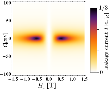
Figure 4: (Color online) Leakage current as a function of transverse external magnetic field and (1,1)-(0,2) energy detuning. Parameters: $B_{z}=0$; further parameter values are the same as for Fig. 2c.

This behavior is shown in Fig. 4. The plot is generated using Eq. (16), with transition rates calculated from the numerically obtained eigenstates of $H_{\rm DQD}$ defined in Eq. (12). The leakage current shown in Fig. 4 displays the hot-spot feature in its dependence on $B_{x}$, and the decreasing current for $\epsilon\gg t$ as predicted in the preceding paragraph.

Figure 4 can be compared to the experimental data of Ref. Pei et al., 2012, where spin-valley blockade was observed and the magnetic field dependence of the leakage current was studied in detail. Importantly, a bent nanotube was used in that experiment, allowing for an interpretation of certain features of the magnetotransport data, but hindering the direct comparison with our results corresponding to a straight CNT. Nevertheless, effects from the bend might be unimportant when the external magnetic field is perpendicular to the plane of the bent CNT, and therefore it makes sense to compare our results to the experimental data corresponding to that case. (Bend-induced effects will be investigated in future work.)

Figure 3c of Ref. Pei et al., 2012 shows the leakage current as a function of transverse external magnetic field ($B_{x}$ in our work) and (1,1)-(0,2) energy detuning ($\epsilon$ in our work). The detuning range where our model, neglecting states lying above the lower-energy doublets, might be relevant is approximately the window $[0,1.5]$ eV. (In our model, this corresponds to $-1.5\,{\rm eV}<\epsilon<0\,{\rm eV}$.) The leakage current measured in this range clearly shows a resonant peak as a function of detuning at $\epsilon\approx 0$, similarly to our result shown in Fig. 4. However, it is hard to judge whether the predicted hot-spot-type dependence of the current on the magnetic field strength $B_{x}$ is present in the experimental data or not. Even if it is, it is certainly blurred by effects not taken into account in our model, perhaps by the interplay of coherent and inelastic interdot tunneling.

For sufficiently strong negative detuning, the leakage current due to coherent hybridization between the (1,1) states and $S_{g}$ might be overcome by the leakage current due to energetically downhill inelastic tunneling processes e.g., assisted by phonon emission. This latter case is discussed in subsection IV.4.

IV.3 Dependence of the leakage current on interdot tunneling

The dependence of the leakage current on the amplitude $t$ of coherent interdot tunneling has not been investigated in the experiment of Ref. Pei et al., 2012. Such a study could confirm the relevance of the blockade-lifting mechanism described in the present work: Our results indicate that the area covered by the current hot spot of Figs. 1c and 2 increases, and the position of the hot spot along the $B_{x}$ axis is shifted towards larger $B_{x}$ values, if the gate-tunable interdot tunneling matrix element $t$ is increased.

IV.4 Regime of inelastic interdot tunneling

As discussed in subsection IV.2, at large (1,1)-(0,2) energy detuning $\epsilon\gg t$, energetically downhill inelastic (e.g., phonon-emission-mediated) tunneling processes might dominate the leakage current. Jouravlev and Nazarov derived a particularly simple formulaJouravlev and Nazarov (2006) for the current in this case, expressed as a function of the unit vectors $\text{\boldmath{$n$}}_{L}$ and $\text{\boldmath{$n$}}_{R}$ associated to the effective magnetic fields in the two dots:

$$I=\frac{e\Gamma_{\rm in}}{4}\left(\text{\boldmath{$n$}}_{L}\times\text{\boldmath{$n$}}_{R}\right)^{2},$$ (24)

where $\Gamma_{\rm in}$ is the inelastic tunneling rate characterizing the $S\to S_{g}$ tunneling process.

We use this formula to evaluate the leakage current as a function of longitudal and transverse external magnetic field for different values of the valley-mixing matrix elements. The results are shown in Fig. 5.

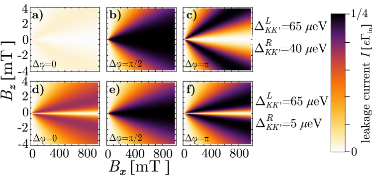
Figure 5: (Color online) The case of inelastic interdot tunneling. Leakage current as a function of transverse ($B_{x}$) and longitudinal ($B_{z}$) external magnetic field for various values of the valley-mixing matrix elements $\Delta_{KK^{\prime}}^{L}$ and $\Delta_{KK^{\prime}}^{R}$ in the two dots. Each row of graphs is obtained using the valley-mixing matrix element magnitudes given at the right end of the row. The difference $\Delta\varphi$ of the complex phases of the valley-mixing matrix elements is shown in each graph at the bottom left corner. Parameters: $g_{s}=2$, $g_{v}=54$, $\Delta_{\rm so}=$370$\;\mu$eV. The plots are obtained by evaluating Eq. (24).

We note that Eq. (24) is valid if the magnitudes of the effective magnetic fields exceed the exchange splitting within the (1,1) charge configuration, i.e., if $\mathcal{B}_{L},\mathcal{B}_{R}\gg t^{2}/\epsilon$.

V Discussion

V.1 Role of electron-electron interaction

Throughout this work we have disregarded the (0,2) triplet states, which are typically energetically separated from the (0,2) ground state $S_{g}$ by a large exchange gap $J_{(0,2)}$Hanson et al. (2007). However, two electrons in a CNT QD might form a Wigner moleculeWunsch (2009); Secchi and Rontani (2009, 2010); von Stecher et al. (2010); Steele et al. (2009); Pecker et al. (2013) due to the strong Coulomb repulsion between electrons and effective one-dimensional nature of the CNT, which implies a drastic reduction of the exchange gap $J_{(0,2)}$ in a Pauli-blockaded DQD. Our description of the current hot spot effect, which disregards the (0,2) triplet states, is valid only if the hybridization between the (1,1) states and the (0,2) triplet states is negligible, i.e., if $t\ll J_{(0,2)}$. This seems to be the case in the spin-valley blockade experiments of Churchill et al.Churchill et al. (2009a, b). The (0,2) exchange gap is very large, comparable to the fundamental gap of the CNT, in the experiments reported in Refs. Pei et al., 2012; Laird et al., 2013, where n-p type DQDs are used.

Another mechanism not taken into account in our model is intervalley Coulomb scatteringAndo (2006); Wunsch (2009); Secchi and Rontani (2009); Weiss et al. (2010); von Stecher et al. (2010); Secchi and Rontani (2013); Pecker et al. (2013); Cleuziou et al. (2013), arising from the short-range (on-site) contribution of the electron-electron interaction. This mechanism can mix the (0,2) singlet ground state with higher-lying (0,2) states. Neglecting this mixing is appropriate as long as the energy scale of the corresponding intervalley Coulomb matrix elements is much smaller than the spin-orbit gap $\Delta_{\rm so}$ separating the states in question.

V.2 Relevance of the results

The fact that the valley-mixing matrix elements influence the shape of the current hot spot might be helpful to experimentally identify the magnitudes and the relative phase of the complex matrix elements $\Delta_{KK^{\prime}}^{L}$ and $\Delta_{KK^{\prime}}^{R}$. Spatial inhomogeneities of valley-mixing effects play an important role in schemes proposed recently for electrical manipulation of single-electron valley- and spin-valley qubits in CNTsFlensberg and Marcus (2010); Pályi and Burkard (2011). A spin-valley blockade measurement in the considered parameter range could be used to explore such inhomogeneities. Furthermore, a difference between the valley-mixing matrix elements $\Delta_{KK^{\prime}}^{L}$ and $\Delta_{KK^{\prime}}^{R}$ and the corresponding effective magnetic fields $\text{\boldmath{$\mathcal{B}$}}_{L}$ and $\text{\boldmath{$\mathcal{B}$}}_{R}$ allows for coherent control of singlet-triplet spin-valley qubits, in a similar fashion as a spatially varying hyperfine or external magnetic field allows for singlet-triplet spin qubit manipulationPetta et al. (2005).

Our results are relevant for blockade-based experimental applications. One example is spin-valley qubit initialization and readoutPei et al. (2012); Laird et al. (2013). Another example is the dc electronic detectionOhm et al. (2012) of the motion of a suspended CNT that acts as a string-like mechanical resonator, a scheme which is based on the interaction between the spin-valley qubit and the bending phonon modes Rudner and Rashba (2010); Pályi et al. (2012). For both applications, it is essential that the leakage current is small in the absence of ac driving. In this work, we have identified regions in the parameter space where the leakage current is nonperturbatively large even in the absence of ac driving; qubit initialization/readout and qubit-based nanomechanical motion detection is possible only outside this parameter regime.

V.3 Conclusion

In conclusion, we have shown that valley-mixing, due to e.g., short-range impurities, can completely lift the spin-valley blockade and hence induce a large leakage current in carbon nanotube double quantum dots, if assisted by an appropriately tuned external magnetic field applied transversally to the tube axis. Measurement of the magnetic field dependence of the leakage current could provide information about the spatial variation of the valley-mixing matrix element. Our study establishes the parameter range (magnetic field vector, interdot tunneling, valley-mixing matrix elements) where weakly disordered CNT DQDs are suited for blockade-based experimental applications such as qubit initialization/readout and nanomechanical motion detection.