A multi-dimensional numerical scheme for two-fluid Relativistic MHD

Abstract

The paper describes an explicit multi-dimensional numerical scheme for Special Relativistic Two-Fluid Magnetohydrodynamics of electron-positron plasma and a suit of test problems. The scheme utilizes Cartesian grid and the third order WENO interpolation. The time integration is carried out using the third order TVD method of Runge-Kutta type, thus ensuring overall third order accuracy on smooth solutions. The magnetic field is kept near divergence-free by means of the method of generalized Lagrange multiplier. The test simulations, which include linear and non-linear continuous plasma waves, shock waves, strong explosions and the tearing instability, show that the scheme is sufficiently robust and confirm its accuracy.

1 Introduction

It is now well recognized that magnetic fields play a very important role in many astrophysical phenomena and in particular in those involving relativistic outflows. The magnetic fields are likely to be involved in launching, powering and collimation of such outflows. The dynamics of relativistic magnetized plasma can be studied using diverse mathematical frameworks. The most developed one so far is the single fluid ideal relativistic Magnetohydrodynamics (RMHD). During the last decade, an impressive progress has been achieved in developing robust and efficient computer codes for integration of its equations. Only within a scope of proper review one can acknowledge the numerous contributions made by many different research groups and individuals. This framework is most suitable for studying large-scale macroscopic motions as it does not require to resolve the microphysical scales for numerical stability. One of its obvious disadvantages is that it allows only numerical dissipation. While at shocks this is not of a problem, the dissipation observed in simulations at other locations may be questionable. This becomes more of an issue as ever growing body of evidence suggests the importance of magnetic dissipation associated with magnetic reconnection in dynamics of highly magnetized relativistic plasma. The framework of resistive RMHD allows to incorporate this magnetic dissipation but the inevitably phenomenological nature of its Ohm’s law puts constraints on its robustness. It is not yet clear how much progress can be achieved in this direction.

At the other extreme is the particle dynamics, describing the motion of individual charges in their collective electromagnetic field. The so-called Particle-in-Cell (PIC) numerical approach has been extremely productive in studying the micro-physics of relativistic collisionless shock waves and magnetic reconnection. The numerical stability considerations require PIC codes to resolve the scales of plasma oscillations. The accuracy considerations can be even more demanding, pushing towards the particle gyration scales. The accuracy of PIC simulations also depends on the number of macro-particles and rather weakly, with the numerical noise level being inversely proportional of the square root of the number. These features make this approach less suitable for studying macroscopic phenomena and only few examples of such simulations can be found in literature (e.g. Arons et al., 2005; Spitkovsky & Arons, 2002).

Somewhere in between there lays the multi-fluid approximation, where plasma is modeled as a collection of several inter-penetrating charged and neutral fluids, coupled via macroscopic electromagnetic field and inter-fluid friction. Undoubtedly, this approach is not as comprehensive in capturing the microphysics of collisionless plasma as the particle dynamics (and kinetics). However, it does this better than the single fluid MHD. In particular, it captures the collective interaction between positive and negative charges which results in plasma waves with frequencies above the plasma frequency. Compared to the resistive MHD, the generalized Ohm’s law of the multi-fluid approximations takes into account the finite inertia of charged particles. From the numerical prospective, the potential of this framework is not clear. By the present time, there has been only a very limited effort to explore it. Zenitani et al. (2009a, b) used this approach for studying the relativistic magnetic reconnection, Amano & Kirk (2013) for studying the termination shocks of pulsar winds, and Kojima & Oogi (2009) tried to construct two-fluid models of steady-state pulsar magnetospheres. The ability, or the lack of it, to describe accurately the magnetic reconnection is probably the most important issue. Zenitani et al. (2009a) concluded that the inertial terms make a significant contribution to the reconnection electric field, even exceeding that of the friction term, which represents the resistivity. This hints that the inertial terms can play an important role in driving the magnetic reconnection. On the other hand, they have also found that the outcome strongly depends on the model of resistivity. Thus, the reconnection issue remains widely open. Another issue is the required numerical resolution. Zenitani et al. (2009a, b) set the grid scale to be comparable to the electron gyration radius. If such high resolution is indeed required then it will be easier just to do PIC simulations. Only if much lower resolution is sufficient, the multi-fluid approach can be advantageous when it comes to macroscopic simulations.

The aforesaid works on the relativistic multi-fluid numerical simulations neither described in details the design of their numerical schemes nor presented test simulations demonstrating their robustness and accuracy. Zenitani et al. (2009a, b) state that they use a “modified Lax-Wendroff scheme”, which employs artificial viscosity, and comment that this is a “bottleneck” of their code. In particular, they find that the contribution of the artificial viscosity to the reconnection electric field is comparable to other contributions. In this paper, we present a high-order accurate Godunov-type scheme for the two-fluid RMHD which does not involve such artificial terms. As a first step, we constrain ourselves with the Special Relativistic framework and the case of pure electron-positron plasma. The scheme utilizes the third order WENO interpolation and the time integration is carried out using the third order TVD method of Runge-Kutta type, thus ensuring overall third order accuracy on smooth solutions. In order to keep the magnetic field divergence-free we employ the method of generalized Lagrange multiplier. The code is parallelized using MPI. We also present a suit of one-dimensional and multi-dimensional test problems and the results of our test simulations. The code is parallelized using MPI. It can be provided by the authors on request.

2 3+1 Special Relativistic electron-positron two-fluid MHD

In the multi-fluid approximation, it is assumed that plasma consists of several interacting fluids, one per each kind of particles involved, and the electromagnetic field. Charged fluids interact with each other electromagnetically and via the so-called inter-fluid friction. The coupling between a fluid of electrically neutral particles and other fluids is only via the inter-fluid friction. Given such understanding, the system of multi-fluid approximation consists of the Maxwell equations and copies of the usual single fluid equations, one per each involved fluid, augmented with the force terms describing these interactions. The fluid equations may be derived via averaging of the corresponding kinetic equations (e.g. Goedbloed & Poedts, 2004).

In one form or another, the equations of relativistic two-fluid MHD were used by many researchers, going back to the work by Akhiezer & Polovin (1956). Following Zenitani et al. (2009a) we adopt the 3+1 Special Relativistic equations originated from the covariant formulation by Gurovich & Solov’ev (1986). In a global inertial frame with time-independent coordinate grid, the equations of two-fluid RMHD include the continuity equations

$$\partial_{t}(\rho_{\pm}\gamma_{\pm})+\nabla_{i}(\rho_{\pm}u_{\pm}^{i})=0\,,$$ (1)

the energy equations

$$\partial_{t}(w_{\pm}\gamma_{\pm}^{2}-p_{\pm})+\nabla_{i}(w_{\pm}\gamma_{\pm}u^{i}_{\pm})=(j^{i}_{\pm}E_{i})\,\pm\,\varkappa_{\mbox{\scriptsize f}}c^{2}n_{+}n_{-}(\gamma_{-}-\gamma_{+})\,,$$ (2)

the momentum equations

$$\partial_{t}\left((w_{\pm}/c^{2})\gamma_{\pm}u_{\pm}^{s}\right)+\nabla_{i}((w_{\pm}/c^{2})u^{i}_{\pm}u^{s}_{\pm}+g^{is}p_{\pm})=q_{\pm}E^{s}+\frac{1}{c}e^{sik}j^{\pm}_{i}B_{k}\,\pm\,\varkappa_{\mbox{\scriptsize f}}n_{+}n_{-}(u^{s}_{-}-u^{s}_{+})\,,$$ (3)

and the Maxwell equations

$$\nabla_{i}B^{i}=0\,,$$ (4)

$$\frac{1}{c}\partial_{t}B^{s}+e^{sik}\partial_{i}E_{k}=0\,,$$ (5)

$$\nabla_{i}E^{i}=4\pi(q_{+}+q_{-})\,,$$ (6)

$$\frac{1}{c}\partial_{t}E^{s}-e^{sik}\partial_{i}B_{k}=-\frac{4\pi}{c}(j^{s}_{+}+j^{s}_{-})\,.$$ (7)

We apply these to the case of electron-positron plasma, so $n_{\pm}$ is the proper number density of positrons and electrons (as measured in the rest frame of the positron and electron fluids respectively), $\rho_{\pm}=m_{\mbox{\scriptsize e}}n_{\pm}$ is the proper mass density, $\gamma_{\pm}$ is the Lorentz factor, $\mn@boldsymbol{u}_{\pm}=\gamma_{\pm}\mn@boldsymbol{v}_{\pm}$ are the spatial components of 4-velocity, $w_{\pm}$ is the relativistic enthalpy, $p_{\pm}$ is the isotropic thermodynamic pressure, $q_{\pm}=\pm e\gamma_{\pm}n_{\pm}$ is the electric charge density, $\mn@boldsymbol{j}_{\pm}=\pm en_{\pm}\mn@boldsymbol{u}_{\pm}$ is the electric current density, $g^{ij}$ is the metric tensor of space, $e^{ijk}$ is the Levi-Civita tensor of space, and $c$ is the speed of light. The last two terms in Eqs.2 and 3 describe the internal friction between the two fluids. The 4-scalar $\varkappa_{\mbox{\scriptsize f}}$ is called the dynamic coefficient of this friction. These equations have to be supplemented by equations of state (EOS), e.g. the polytropic EOS

$$w_{\pm}=n_{\pm}m_{e}c^{2}+\Gamma p_{\pm}/(\Gamma-1)\,,$$ (8)

where $\Gamma$ is the ratio of specific heats.

By subtracting the momentum equations for the positron and electron fluids, one obtains the so-called generalized Ohm law of the two-fluid MHD:

$$\partial_{t}\left(\sum\limits_{\pm}\pm(w_{\pm}/c^{2})\gamma_{\pm}u_{\pm}^{s}\right)+\nabla_{i}\left(\sum\limits_{\pm}\pm((w_{\pm}/c^{2})u^{i}_{\pm}u^{s}_{\pm}+p_{\pm}g^{is})\right)=e\tilde{n}\left(E^{s}+\frac{1}{c}e^{sik}v_{i}B_{k}\right)-\frac{2\varkappa_{\mbox{\scriptsize f}}}{e}(n_{+}j^{s}_{-}+n_{-}j^{s}_{+})\,,$$ (9)

In this equation,

$$\tilde{n}=n_{+}\gamma_{+}+n_{-}\gamma_{-}$$ (10)

is the total number density of charged particles as measured in the laboratory frame and

$$\mn@boldsymbol{v}=\frac{n_{+}\mn@boldsymbol{u}_{+}+n_{-}\mn@boldsymbol{u}_{-}}{\tilde{n}}=\frac{\mn@boldsymbol{j}_{+}-\mn@boldsymbol{j}_{-}}{e\tilde{n}}$$ (11)

is their average velocity in this frame. In general, the internal friction of a single fluid, not introduced in our model, leads to viscosity and the internal friction between two charged fluids to resistivity. In order to understand the properties of this resistivity, consider the Ohm’s law in the plasma frame (where $\mn@boldsymbol{v}=0$) and ignore the inertial terms (the terms in the left-hand side of the generalized Ohm’s law). This gives us

$$\mn@boldsymbol{E}=\frac{2\varkappa_{\mbox{\scriptsize f}}}{e^{2}\tilde{n}}(n_{+}\mn@boldsymbol{j}_{-}+n_{-}\mn@boldsymbol{j}_{+})\,.$$ (12)

Since $\mn@boldsymbol{v}=0$, we have $\mn@boldsymbol{j}_{+}=\mn@boldsymbol{j}_{-}=\mn@boldsymbol{j}/2$, where $\mn@boldsymbol{j}=\mn@boldsymbol{j}_{+}+\mn@boldsymbol{j}_{-}$ is the total electric current, and hence obtain the usual Ohm’s law

$$\mn@boldsymbol{j}=\sigma\mn@boldsymbol{E}\,,$$ (13)

with the scalar conductivity coefficient

$$\sigma=\frac{e^{2}}{\varkappa_{\mbox{\scriptsize f}}}\left(\frac{\tilde{n}}{n_{+}+n_{-}}\right)\,.$$ (14)

The corresponding resistivity coefficient is defined as $\eta=1/4\pi\sigma$.

For the purpose of mathematical analysis and computations, it is best to deal with dimensionless equations. Denote as $B_{0}$ the characteristic value of magnetic (and electric) field, as $T_{0}$ the characteristic time scale, as $L_{0}=cT_{0}$ the characteristic length scale, and as $n_{0}$ the characteristic number density of particles. Then the characteristic scale for $\rho$ is $m_{\mbox{\scriptsize e}}n_{0}$ and the characteristic scale for $w$ and $p$ is $m_{\mbox{\scriptsize e}}c^{2}n_{0}$. The corresponding dimensionless equations of the two-fluid electron-positron RMHD are

$$\partial_{t}(n_{\pm}\gamma_{\pm})+\nabla_{i}(n_{\pm}u_{\pm}^{i})=0\,,$$ (15)

$$\partial_{t}(w_{\pm}\gamma_{\pm}^{2}-p_{\pm})+\nabla_{i}(w_{\pm}\gamma_{\pm}u^{i}_{\pm})=\pm\frac{1}{\mathcal{K}_{\mbox{\scriptsize m}}}n_{\pm}(u^{i}_{\pm}E_{i})\,\pm\,\frac{1}{\mathcal{K}_{\mbox{\scriptsize f}}}n_{+}n_{-}(\gamma_{-}-\gamma_{+})\,,$$ (16)

$$\partial_{t}\left(w_{\pm}\gamma_{\pm}u_{\pm}^{s}\right)+\nabla_{i}(w_{\pm}u^{i}_{\pm}u^{s}_{\pm}+g^{is}p_{\pm})=\pm\frac{1}{\mathcal{K}_{\mbox{\scriptsize m}}}n_{\pm}\gamma_{\pm}(E^{s}+e^{sik}v^{\pm}_{i}B_{k})\,\pm\,\frac{1}{\mathcal{K}_{\mbox{\scriptsize f}}}n_{+}n_{-}(u^{s}_{-}-u^{s}_{+})\,,$$ (17)

$$\nabla_{i}B^{i}=0\,,$$ (18)

$$\partial_{t}B^{s}+e^{sik}\partial_{i}E_{k}=0\,,$$ (19)

$$\nabla_{i}E^{i}=\frac{1}{\mathcal{K}_{\mbox{\scriptsize q}}}(n_{+}\gamma_{+}-n_{-}\gamma_{-})\,,$$ (20)

$$\partial_{t}E^{s}-e^{sik}\partial_{i}B_{k}=-\frac{1}{\mathcal{K}_{\mbox{\scriptsize q}}}(n_{+}u_{+}^{s}-n_{-}u^{s}_{-})\,.$$ (21)

The three dimensionless parameters in these equations are

$$\mathcal{K}_{\mbox{\scriptsize q}}=\frac{B_{0}}{4\pi eL_{0}n_{0}}\,,\quad\mathcal{K}_{\mbox{\scriptsize m}}=\frac{m_{\mbox{\scriptsize e}}c^{2}}{eB_{0}L_{0}}\,,\quad\mathcal{K}_{\mbox{\scriptsize f}}=\frac{m_{\mbox{\scriptsize e}}c}{\varkappa_{\mbox{\scriptsize f}}n_{0}L_{0}}\,.$$ (22)

The dimensionless polytropic EOS is

$$w_{\pm}=n_{\pm}+\Gamma p_{\pm}/(\Gamma-1)\,.$$ (23)

Table 1: Important plasma parameters in dimensional and dimensionless form. Here the magnetic field $\hat{B}$ is measured in the plasma rest frame, $w=w_{+}+w_{-}$, $p=p_{+}+p_{-}$ and $n=n_{+}+n_{-}$.

Name	Dimensional expression	Dimensionless expression
plasma frequency	$\Omega_{\mbox{\scriptsize p}}^{2}=\frac{4\pi e^{2}n^{2}c^{2}}{w}$	$\Omega_{\mbox{\scriptsize p}}^{2}=\frac{1}{\mathcal{K}_{\mbox{\scriptsize q}}\mathcal{K}_{\mbox{\scriptsize m}}}\left(\frac{n^{2}}{w}\right)$
skin depth	$\lambda_{\mbox{\scriptsize s}}=\frac{c}{\Omega_{\mbox{\scriptsize p}}}$	$\lambda_{\mbox{\scriptsize s}}=\left(\frac{1}{\Omega_{\mbox{\scriptsize p}}}\right)$
magnetization $\beta$	$\beta=\frac{8\pi p}{\hat{B}^{2}}$	$\beta=\frac{\mathcal{K}_{\mbox{\scriptsize m}}}{\mathcal{K}_{\mbox{\scriptsize q}}}\left(\frac{2p}{\hat{B}^{2}}\right)$
magnetization $\sigma_{\mbox{\scriptsize m}}$	$\sigma_{\mbox{\scriptsize m}}=\frac{\hat{B}^{2}}{4\pi w}$	$\sigma_{\mbox{\scriptsize m}}=\frac{\mathcal{K}_{\mbox{\scriptsize q}}}{\mathcal{K}_{\mbox{\scriptsize m}}}\left(\frac{\hat{B}^{2}}{w}\right)$
gyration radius	$R_{\mbox{\scriptsize g}}=\frac{m_{\mbox{\scriptsize e}}c^{2}}{e\hat{B}}\left(\left(\frac{w-p}{\rho c^{2}}\right)^{2}-1\right)^{1/2}$	$R_{\mbox{\scriptsize g}}=\frac{\mathcal{K}_{\mbox{\scriptsize m}}}{\hat{B}}\left(\left(\frac{w-p}{n}\right)^{2}-1\right)^{1/2}$

We write the dimensionless two-fluid equations in the form which focuses on their mathematical structure. Although this somewhat hides the physical origin of the system, all the important plasma parameters can be easily recovered when this is needed. Some of them are listed in Table 1. The parameters $\mathcal{K}_{\mbox{\scriptsize m}}$, $\mathcal{K}_{\mbox{\scriptsize f}}$, and $\mathcal{K}_{\mbox{\scriptsize q}}$ also allow simple physical interpretation. $\mathcal{K}_{\mbox{\scriptsize m}}$ is the ratio of the particle rest mass energy $m_{\mbox{\scriptsize e}}c^{2}$ to the potential drop $eB_{0}L_{0}$ in the electric field of strength $E_{0}=B_{0}$ over the characteristic length scale of the problem. Obviously, this is a measure of the magnetic field strength. $\mathcal{K}_{\mbox{\scriptsize f}}$ is the ratio of the relaxation time scale $T_{\mbox{\scriptsize f}}=m_{\mbox{\scriptsize e}}/n_{0}\varkappa_{\mbox{\scriptsize f}}$ in plasma of number density $n_{0}$ and the light-crossing time scale $T_{0}=L_{0}/c$. $\mathcal{K}_{\mbox{\scriptsize q}}$ is the inverse ratio of $n_{0}$ and the Goldreich-Julian number density of charged particles

$$n_{\mbox{\scriptsize GJ}}=B_{0}/4\pi eL_{0}\,.$$ (24)

From the expressions for the plasma magnetizations $\beta$ and $\sigma_{\mbox{\scriptsize m}}$ given in Table 1 it is easy to see how to setup two-fluid problems corresponding to single-fluid RMHD problems, e.g. the test problems of Komissarov (1999). One can use the same dimensionless values for the total thermodynamic pressure and density, but scale the electromagnetic field by the factor of $\sqrt{\mathcal{K}_{\mbox{\scriptsize m}}/\mathcal{K}_{\mbox{\scriptsize q}}}$.

By summing together the energy equations Eqs.16 and then utilizing the Maxwell equations one obtains the conservation law for the total energy,

$$\partial_{t}\left(\sum\limits_{\pm}(w_{\pm}\gamma_{\pm}^{2}-p_{\pm})+\frac{\mathcal{K}_{\mbox{\scriptsize q}}}{2\mathcal{K}_{\mbox{\scriptsize m}}}(B^{2}+E^{2})\right)+\nabla_{i}\left(\sum\limits_{\pm}w_{\pm}\gamma_{\pm}u^{i}_{\pm}+\frac{\mathcal{K}_{\mbox{\scriptsize q}}}{\mathcal{K}_{\mbox{\scriptsize m}}}e^{ijk}E_{j}B_{k}\right)=0\,.$$ (25)

Similarly, one finds the total momentum conservation law

$$\partial_{t}\left(\sum\limits_{\pm}w_{\pm}\gamma_{\pm}u_{\pm}^{s}+\frac{\mathcal{K}_{\mbox{\scriptsize q}}}{\mathcal{K}_{\mbox{\scriptsize m}}}e^{sjk}E_{j}B_{k}\right)+\nabla_{i}\left(\sum\limits_{\pm}(w_{\pm}u^{i}_{\pm}u^{s}_{\pm}+p_{\pm}g^{is})+\frac{\mathcal{K}_{\mbox{\scriptsize q}}}{\mathcal{K}_{\mbox{\scriptsize m}}}\left(-E^{i}E^{s}-B^{i}B^{s}+\frac{1}{2}(B^{2}+E^{2})g^{is}\right)\right)=0\,.$$ (26)

By subtracting the dimensionless momentum equations for the positron and electron fluids one obtains the dimensionless generalized Ohm law of the two-fluid MHD:

$$\partial_{t}\left(\sum\limits_{\pm}\pm w_{\pm}\gamma_{\pm}u_{\pm}^{s}\right)+\nabla_{i}\left(\sum\limits_{\pm}\pm(w_{\pm}u^{i}_{\pm}u^{s}+p_{\pm}g^{is})\right)=\frac{1}{\mathcal{K}_{\mbox{\scriptsize m}}}\tilde{n}(E^{s}+e^{sik}v_{i}B_{k})+\frac{2}{\mathcal{K}_{\mbox{\scriptsize f}}}n_{+}n_{-}(u^{s}_{-}-u^{s}_{+})\,.$$ (27)

In this equation, $\tilde{n}=n_{+}\gamma_{+}+n_{-}\gamma_{-}$ is the total number density of charged particles as measured in the laboratory frame and $v^{i}=(n_{+}\gamma_{+}v^{i}_{+}+n_{-}\gamma_{-}v^{i}_{-})/\tilde{n}$ is their average velocity in this frame. Subtracting the dimensionless energy equations, we obtain the time component of the generalized Ohm’s law

$$\partial_{t}\left(\sum\limits_{\pm}\pm(w_{\pm}\gamma_{\pm}^{2}-p_{\pm})\right)+\nabla_{i}\left(\sum\limits_{\pm}\pm(w_{\pm}\gamma_{\pm}u^{i}_{\pm})\right)=\frac{1}{\mathcal{K}_{\mbox{\scriptsize m}}}\tilde{n}(v^{i}E_{i})+\frac{2}{\mathcal{K}_{\mbox{\scriptsize f}}}n_{+}n_{-}(\gamma_{-}-\gamma_{+})\,.$$ (28)

3 Numerical method

From the analysis of Sec.2, it follows that there is a significant freedom in the selection of mathematically equivalent closed system of equations to describe the dynamics of two-fluid plasma. However for numerical integration, it is often advantageous to select equations which do not involve source terms. In this case, one can utilize the ability of modern shock capturing schemes to preserve conserved quantities down to the computer rounding error, which is important for problems involving discontinuities. For this reason, the fluid equations utilized in our numerical scheme include Eqs. 15, 25 and 26. The system is closed by including the generalized Ohm’ law, Eqs. 27 and 28, and the so-called augmented Maxwell equations, which are described below.

3.1 Augmented Maxwell Equations

In order to keep the magnetic field divergence free and to ensure that the Gauss law is satisfied as well, we use the so-called Generalized Lagrange Multiplier method (Munz et al., 2000; Dedner et al., 2002; Komissarov, 2007). To this end, the Maxwell equations are modified in such a way that all four of them become dynamic. Namely,

$$\partial_{t}\Phi+\nabla_{i}B^{i}=-\kappa\Phi\,,$$ (29)

$$\partial_{t}B^{s}+e^{sik}\partial_{i}E_{k}+\nabla^{s}{\Phi}=0\,,$$ (30)

$$\partial_{t}\Psi+\nabla_{i}E^{i}=\frac{1}{\mathcal{K}_{\mbox{\scriptsize q}}}(n_{+}\gamma_{+}+n_{-}\gamma_{-})-\kappa\Psi\,,$$ (31)

$$\partial_{t}E^{s}-e^{sik}\partial_{i}B_{k}+\nabla^{s}\Psi=-\frac{1}{\mathcal{K}_{\mbox{\scriptsize q}}}(n_{+}u_{+}^{s}-n_{-}u^{s}_{-})\,,$$ (32)

where the scalars $\Phi$ and $\Psi$ are two additional dynamic variables and $\kappa$ is a positive constant, which determines the rate of decay of $\nabla_{i}B^{i}$ and $\nabla_{i}E^{i}-(1/\mathcal{K}_{\mbox{\scriptsize q}})(n_{+}\gamma_{+}+n_{-}\gamma_{-})$. Obviously, the resultant equations are of the same structure as the fluid equations and hence they can be discretized in exactly the same way. This property greatly simplifies computational algorithms and coding.

3.2 Finite-difference conservative scheme

In our numerical scheme, we integrate Eqs. 15, 25, 26, 27, 28, and the augmented Maxwell equations 29-32. Taken together, they can be written as a single phase vector equation of the form

$$\frac{\partial{\cal Q}}{\partial t}+\frac{\partial{\cal F}^{m}}{\partial x^{m}}={\cal S}\,,$$ (33)

where ${\cal Q}$ is the vector of conserved variables, ${\cal F}^{m}$ is the vector of fluxes in the $x^{m}$ direction and ${\cal S}$ is the vector of source terms. When $\{x^{m}\}$ are Cartesian coordinates, and this is the only case we have coded so far, one can simply replace $\nabla_{m}$ with $\partial_{m}$ and hence read the components of ${\cal Q}$, ${\cal F}^{m}$ and ${\cal S}$ directly from the aforesaid equations. Otherwise, these expressions will also involve components of the metric tensor.

Introduce a uniform coordinate grid such that $x^{m}_{i}$ is the coordinate of the center of the $i$th cell, and $x^{m}_{i\pm 1/2}$ are the coordinates of its right and left interfaces. Replace, the continuous function $Q$ with a discrete function defined at the cell centers and the continuous functions $F^{m}$ with discrete functions defined at the centers of $x^{m}$ cell interfaces. Finally, replace $\partial_{m}{{\cal F}^{m}}$ with the finite difference approximations:

$${\cal D\!F}_{i,j,k}=\frac{{\cal F}^{1}_{i+1/2,j,k}-{\cal F}^{1}_{i-1/2,j,k}}{\Delta x^{1}}+\frac{{\cal F}^{2}_{i,j+1/2,k}-{\cal F}^{2}_{i-1/2,j,k}}{\Delta x^{2}}+\frac{{\cal F}^{3}_{i,j,k+1/2}-{\cal F}^{3}_{i,j,k-1/2}}{\Delta x^{3}}\,.$$ (34)

As the result Eq.33 becomes a set of coupled ODEs

$$\frac{d{\cal Q}_{i,j,k}}{dt}={\cal L}_{i,j,k}({\cal Q})$$ (35)

where

$${\cal L}_{i,j,k}({\cal Q})=-{\cal D\!F}_{i,j,k}({\cal Q})+S({\cal Q}_{i,j,k})\,.$$ (36)

In this equation, the notation ${\cal D\!F}_{i,j,k}({\cal Q})$ means that, strictly speaking, the argument of ${\cal D\!F}_{i,j,k}$ is the whole of the discrete function ${\cal Q}$ (exactly the same applies to ${\cal L}_{i,j,k}({\cal Q})$). However in reality, only few of its values, in the cells around the $(i,j,k)$-cell, are involved – this defines the scheme stencil.

It is easy to see that, when the equations of the system (35) are integrated simultaneously, the quantities

$$\sum\limits_{i,j,k}{\cal Q}_{i,j,k}$$ (37)

are conserved down to rounding error. Any larger variation may only be due to a non-vanishing source term in (35) or a non-vanishing total flux of the quantity through the boundary of the computational domain. In this sense, this finite difference scheme is conservative.

3.3 Third-order WENO interpolation

In order to calculate fluxes at the cell interfaces, and hence ${\cal D\!F}_{i,j,k}({\cal Q})$, we use the third-order weighted essentially non-oscillatory (WENO) interpolation developed by Liu et al. (1994), in the improved form proposed by Yamaleev & Carpenter (2009). However, instead of interpolating the conserved variables we prefer to interpolate the primitive ones, ${\cal P}=(n_{\pm},\,p_{\pm},\,u^{s}_{\pm},\,E^{s},\,B^{s},\,\Phi,\,\Psi)$. The benefit of this is twofold. Firstly, this reduces by the factor of two the number of required conversions of conserved variables into the primitive ones. Indeed, in order to compute the flux vector from the vector of conserved variables one would have to convert the latter into the vector of primitive variables first. This would have to be done twice per each interface. Secondly, this ensures physically meaningful interpolated phase states.

The aim of the interpolation is to provide us with phase states immediately to the left and right of each cell interface given those at the cell centers. In the third order WENO interpolation, the interface values are found via a convex linear combination of two linear interpolants, which provides third order accuracy on smooth solutions. For the $i$-th cell the interpolants are

$${\cal P}_{r}(x)={\cal P}_{i}+\frac{\Delta{\cal P}_{r}}{\Delta x}(x-x_{i})\quad\mbox{and}\quad{\cal P}_{l}(x)={\cal P}_{i}+\frac{\Delta{\cal P}_{l}}{\Delta x}(x-x_{i})\,,$$

where $\Delta{\cal P}_{r}={\cal P}_{i+1}-{\cal P}_{i}$ and $\Delta{\cal P}_{l}={\cal P}_{i}-{\cal P}_{i-1}$. Here we consider only one of the coordinate directions and omit indexes for others. Their convex combination is

$${\cal P}(x)=w_{r}{\cal P}_{r}(x)+w_{l}{\cal P}_{l}(x)\,,$$

where $w_{r,l}>0$ and $w_{r}+w_{l}=1$. These conditions on the weights are satisfied when

$$w_{r}=\frac{\alpha_{r}}{\alpha_{r}+\alpha_{l}}\quad\mbox{and}\quad w_{l}=\frac{\alpha_{l}}{\alpha_{r}+\alpha_{l}}\,,$$

where $\alpha_{l,r}>0$. Removing the arbitrary small constant $\epsilon$, artificially introduced in Yamaleev & Carpenter (2009) in order to avoid division by zero during the calculations of $\alpha_{r,l}$, and somewhat rearranging their equations, we find the interpolated values of ${\cal P}$ at the left and right interfaces of the cell

$${\cal P}_{i\pm 1/2}={\cal P}_{i}\pm(a_{r,l}\Delta{\cal P}_{r,l}+\frac{1}{2}a_{l,r}\Delta{\cal P}_{l,r})/(2a_{r,l}+a_{l,r})\,,$$ (38)

where

$$a_{r,l}=\Delta{\cal P}_{l,r}^{2}\left(\Delta{\cal P}_{r,l}^{2}+(\Delta{\cal P}_{r}+\Delta{\cal P}_{l})^{2}\right)\,.$$ (39)

It is easy to verify that Eq.38 yields ${\cal P}_{i\pm 1/2}={\cal P}_{i}$ when either $\Delta{\cal P}_{l}=0$ or $\Delta{\cal P}_{r}=0$. Thus, one can put

$${\cal P}_{i\pm 1/2}={\cal P}_{i}\quad\mbox{if}\quad\Delta{\cal P}_{l}\Delta{\cal P}_{r}=0\,.$$ (40)

This allows us to avoid the $0/0$ indeterminacy implied by Eqs.38,39, via a simple inspection of data.

3.4 Riemann solver

Using the interpolation described in the previous section, one obtains two phase states, ${\cal P}_{\mbox{\scriptsize L}}$ and ${\cal P}_{\mbox{\scriptsize R}}$, for each cell interface. The state ${\cal P}_{\mbox{\scriptsize L}}$ is obtained via the WENO interpolation inside the cell to the left of the interface, as described in the previous section, where it coresponds to ${\cal P}_{i+1/2}$, whereas the state ${\cal P}_{\mbox{\scriptsize R}}$ is obtained via the interpolation inside the cell to the right of the interface, where it coresponds to ${\cal P}_{i-1/2}$. This defines 1D Riemann problems whose solutions can be used to compute the interface fluxes required in Eq.34. Finding exact and even linearized solutions of Riemann problems for complicated systems of equations can be rather expensive. In such cases, it makes sense to utilize methods which use minimum amount of information about there characteristic properties, like the Lax-Friedrich flux, which requires to know only the highest wave speed of the system and purely for the stability consideration. Since in the relativistic framework the highest speed equals to the speed of light, the latter can replace the former in the Lax-Friedrich flux, leading to the equation

$${\cal F}_{\mbox{\scriptsize LF}}=\frac{1}{2}({\cal F}_{\mbox{\scriptsize L}}+{\cal F}_{\mbox{\scriptsize R}})-\frac{1}{2}({\cal Q}_{\mbox{\scriptsize R}}-{\cal Q}_{\mbox{\scriptsize L}})\,,$$ (41)

where $\{{\cal F}_{\mbox{\scriptsize L}},{\cal F}_{\mbox{\scriptsize R}}\}$ and $\{{\cal Q}_{\mbox{\scriptsize L}},{\cal Q}_{\mbox{\scriptsize R}}\}$ are the vectors of fluxes and conserved variables corresponding to the left and the right phase states respectively (e.g. ${\cal F}_{\mbox{\scriptsize L}}={\cal F}({\cal P}_{\mbox{\scriptsize L}})$). The second term in the right-hand side of this equation introduces diffusion, which stabilizes numerical solutions. Although this diffusion may be excessive, its negative effect is significantly diminished in smooth regions, when schemes with highly accurate reconstruction are employed.

3.5 Time integration

For the integration of the coupled ODEs given by Eq.35 we use the popular third-order total variation diminishing (TVD) Runge-Kutta scheme by Shu & Osher (1988). The one time-step calculations proceed as follows.

$${\cal Q}^{(1)} = {\cal Q}^{n}+\Delta t{\cal L}({\cal Q}^{n})\,,$$

$${\cal Q}^{(2)} = {\cal Q}^{n}+\frac{\Delta t}{4}\left({\cal L}({\cal Q}^{(1)})+{\cal L}({\cal Q}^{n})\right)\,,$$ (42)

$${\cal Q}^{n+1} = {\cal Q}^{n}+\frac{\Delta t}{6}\left({\cal L}({\cal Q}^{n})+{\cal L}({\cal Q}^{(1)})+4{\cal L}({\cal Q}^{(2)})\right)\,,$$

where ${\cal Q}^{n}$ and ${\cal Q}^{n+1}$ are the values of ${\cal Q}$ at the times $t^{n}$ and $t^{n+1}=t^{n}+\Delta t$, and ${\cal Q}^{(1)}$ and ${\cal Q}^{(2)}$ are two auxiliary vectors. For stability, the time step must satisfy the Courant condition. Since the highest speed of communication in our case is the speed of light, this condition reads $\Delta t=c_{\mbox{\scriptsize n}}\min(\Delta x^{i})$, where $c_{\mbox{\scriptsize n}}<1$. Even smaller time step is required when the source terms are large.

3.6 Conversion of conservative into primitive variables

The recovering of the hydrodynamic primitive variables is carried out in three steps. First we use updated $\mn@boldsymbol{E}$ and $\mn@boldsymbol{B}$ to remove the electromagnetic contributions from the updated total energy and momentum. Second, via adding and subtracting the corresponding conserved variables we recover the energies and momenta of the electron and positron fluids. As the result, for each of the fluids we have the set of five conserved quantities

$${\cal D}=n\gamma,\quad{\cal E}=w\gamma^{2}-p,\quad{\cal M}^{i}=w\gamma^{2}v^{i}\,,$$ (43)

where we dropped $\pm$. This is a set of non-linear equation for the primitive variables $n$, $p$, and $v^{i}$. In the literature, one can find a number of different algorithms for solving these equations. We employ the following simple iterative procedure, developed earlier for our code for relativistic gas dynamics (Falle & Komissarov, 1996). Denoting $w\gamma^{2}$ as $Y$,

$$Y_{k+1}={\cal E}+p_{k},\quad v^{2}_{k+1}={\cal M}^{2}/Y_{k+1}^{2},\quad n_{k+1}={\cal D}/\gamma_{k+1},\quad w_{k+1}=Y_{k+1}/\gamma^{2}_{k+1},\quad p_{k+1}=p(w_{k+1},n_{k+1})\,.$$ (44)

As the initial guess for $p$ we use its value from the previous time step. Depending on how good this initial guess is, it takes between 4 iterations in smooth regions to 20 iterations near shocks for the solution to converge down to eight significant digits.

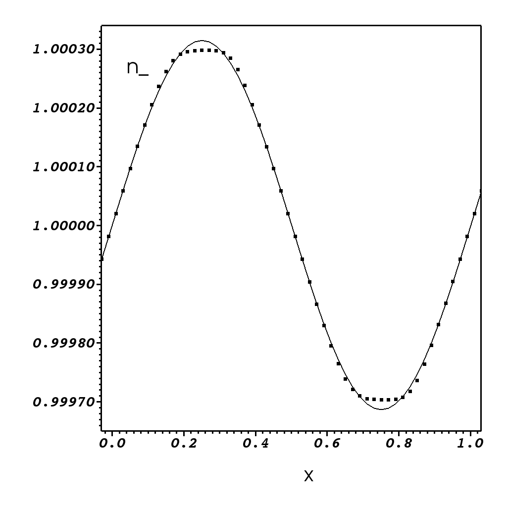
Figure 1: Propagation of small amplitude electrostatic waves. The number density of electrons (left panel) and the electric field (right panel). The continuous lines show the initial solution and the dots show the numerical solution after one period.

4 Test simulations

Many of our test simulations are based on slab-symmetric one-dimensional problems with known exact analytic or semi-analytic solutions. Such problems allow to test not only the 1D version of the code but also the multi-dimensional ones. The latter is achieved simply via using the multi-dimensional codes to solve one-dimensional problems aligned with one of the grid directions. In addition, we used truly multi-dimensional problems for which there is no exact solutions but which have been found useful for testing one-fluid RMHD codes. The simulations have been carried out either on a laptop or/and a workstation with multi-core processors.

In all simulations, the parameter $\kappa$ of the augmented Maxwell equations is fixed at $\kappa=0.1$.

4.1 Electrostatic waves

The two-fluid equations allow additional types of waves compared to the single fluid MHD. The most basic new waves are the electrostatic waves. In relativistic two-fluid MHD with $\mathcal{K}_{\mbox{\scriptsize f}}=\infty$, the properties of linear electrostatic waves were first studied by Sakai & Kawata (1980). Their background solution describes uniform state with zero velocity and electric field. The waves propagate along the magnetic field and perturb only the particle density and the components of velocity and electric field along the magnetic field. Choosing the x axis aligned with the magnetic field, putting $A=\tilde{A}\exp(\mbox{i}(\Omega t-kx))$ for the perturbation and assuming the same thermodynamic parameters for electron and positron fluids, one finds the dispersion relation

$$\Omega^{2}=\Omega_{p}^{2}(1+(k/k_{\mbox{\scriptsize b}})^{2})\,,$$ (45)

where $\Omega_{p}$ is the electron plasma frequency of the uniform background and

$$k_{\mbox{\scriptsize b}}^{2}=\frac{1}{\mathcal{K}_{\mbox{\scriptsize m}}\mathcal{K}_{\mbox{\scriptsize q}}}\left(\frac{2n^{2}_{\mbox{\scriptsize b}}}{\Gamma p_{\mbox{\scriptsize b}}}\right)\,,$$ (46)

where the $n_{\mbox{\scriptsize b}}$ and $p_{\mbox{\scriptsize b}}$ are the background electron (and positron) number density and pressure respectively. For the Fourier amplitudes one has

$$\tilde{n}_{\pm}=n_{\mbox{\scriptsize b}}\left(\frac{k}{\Omega}\right)\tilde{v}^{x}_{\pm}\,$$ (47)

and

$$\tilde{v}^{x}_{\pm}=\pm\mbox{i}\frac{1}{\mathcal{K}_{\mbox{\scriptsize m}}}\frac{n_{\mbox{\scriptsize b}}\Omega}{(\Gamma p_{\mbox{\scriptsize b}}k^{2}-w_{\mbox{\scriptsize b}}\Omega^{2})}\tilde{E}^{x}\,.$$ (48)

Figure 1 shows the results of 1D test simulations based on this solution. The parameters used in this test are $\mathcal{K}_{\mbox{\scriptsize q}}=\mathcal{K}_{\mbox{\scriptsize m}}=1$, $\mathcal{K}_{\mbox{\scriptsize f}}=\infty$, $k=2\pi$, $\Gamma=4/3$, $n_{\mbox{\scriptsize b}}=p_{\mbox{\scriptsize b}}=1$ and $\tilde{E}^{x}=10^{-4}$. The uniform computational grid has 50 cells covering the domain $[0,1]$. One can see that in spite of the relatively low spatial resolution, the numerical solution is quite accurate, particularly for the electromagnetic field. Noticeable errors are observed only in the gas parameters near the turning points of the wave curve.

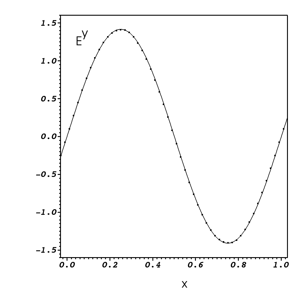
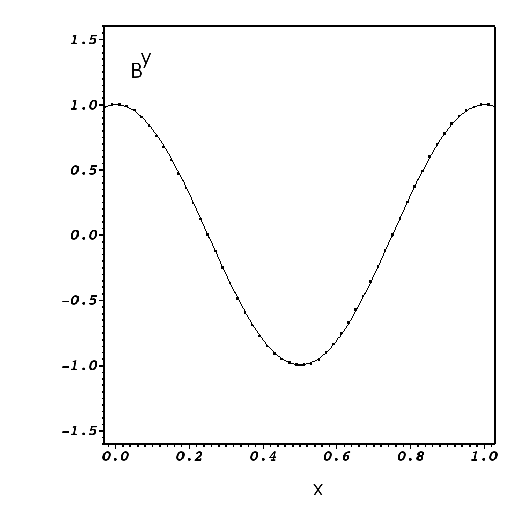
Figure 2: Propagation of circularly polarized “superluminal” waves. The left panel shows $E^{y}$ and the right panel shows $B^{y}$. The continuous lines show the initial solution and the dots show the numerical solution after one period.

Table 2: L1 norm errors in the problem of circularly polarized wave.

$N$	$p_{-}$	$B$	$u_{-}$
50	$9.94\times 10^{-2}$	$2.73\times 10^{-3}$	$3.56\times 10^{-1}$
100	$1.07\times 10^{-2}$	$4.23\times 10^{-4}$	$4.55\times 10^{-2}$
200	$1.23\times 10^{-3}$	$5.81\times 10^{-5}$	$5.32\times 10^{-3}$
400	$1.46\times 10^{-4}$	$7.57\times 10^{-6}$	$6.34\times 10^{-4}$

4.2 Circularly polarized “superluminal” waves.

These are nonlinear harmonic solutions of the two-fluid equations with $\mathcal{K}_{\mbox{\scriptsize f}}=\infty$ (e.g. Max, 1973; Amano & Kirk, 2013). Their background solution describes uniform state with vanishing velocity, magnetic and electric fields and equal densities and pressures of the electron and positron fluids. These waves do not perturb particle density and pressure, as well as the velocity component along the wave vector. The components of vectors normal to the wave vector display pure rotation, whose direction depends on the wave polarization. Choosing the x-axis aligned with the wave vector and putting $A=\tilde{A}\exp(\mbox{i}(\Omega t-kx))$ for the wave of left polarization one finds the dispersion relation

$$\Omega=\Omega_{\mbox{\scriptsize p}}(1+(k/k_{\mbox{\scriptsize b}})^{2})^{1/2},$$ (49)

where $\Omega_{p}$ is the plasma frequency and $k_{\mbox{\scriptsize b}}=1/\Omega_{\mbox{\scriptsize p}}$. The corresponding Fourier amplitudes are related via

$$\tilde{\mn@boldsymbol{u}}_{\perp,\pm}=\pm\frac{1}{\mathcal{K}_{\mbox{\scriptsize m}}}\frac{n_{\mbox{\scriptsize b}}}{kw_{\mbox{\scriptsize b}}}\tilde{\mn@boldsymbol{B}}_{\perp}\,,$$ (50)

$$\tilde{\mn@boldsymbol{E}}_{\perp}=-\mbox{i}\frac{\Omega}{k}\tilde{\mn@boldsymbol{B}}_{\perp}\,,$$ (51)

where as before $n_{\mbox{\scriptsize b}}$ and $w_{\mbox{\scriptsize b}}$ are the unperturbed background electron density and enthalpy respectively. For the right polarization, $A=\tilde{A}\exp(-\mbox{i}(kx-\Omega t))$, Eq.50 is replaced with

$$\tilde{\mn@boldsymbol{u}}_{\perp,\pm}=\mp\frac{1}{\mathcal{K}_{\mbox{\scriptsize m}}}\frac{n_{\mbox{\scriptsize b}}}{kw_{\mbox{\scriptsize b}}}\tilde{\mn@boldsymbol{B}}_{\perp}\,.$$ (52)

Figure 2 shows the results of 1D test simulations, based on the solution for the left polarization wave. The parameters of the problem are $\mathcal{K}_{\mbox{\scriptsize q}}=1$, $\mathcal{K}_{\mbox{\scriptsize m}}=1/(2\pi)^{2}$, $\mathcal{K}_{\mbox{\scriptsize f}}=\infty$, $p_{\mbox{\scriptsize b}}=1/4$, $n_{\mbox{\scriptsize b}}=1$, $\Gamma=4/3$, $v_{\pm}^{x}=0$, $B^{x}=0$ and $k=2\pi$. The corresponding wave phase speed is $v_{\phi}=\sqrt{2}$. The uniform computational grid has 50 cells and covers the domain $[0,1]$. In this figure the continuous lines show the initial solution and the dots show the numerical solution after one wave period, at $t=1/\sqrt{2}$. Table 2 show the L1 norm of the numerical errors for $p_{-}$ and the magnitudes of $B$, and $u_{-}$, all of which should remain constant. The data confirm that the scheme is third order accurate.

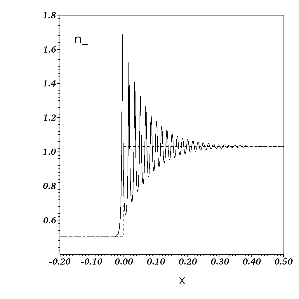
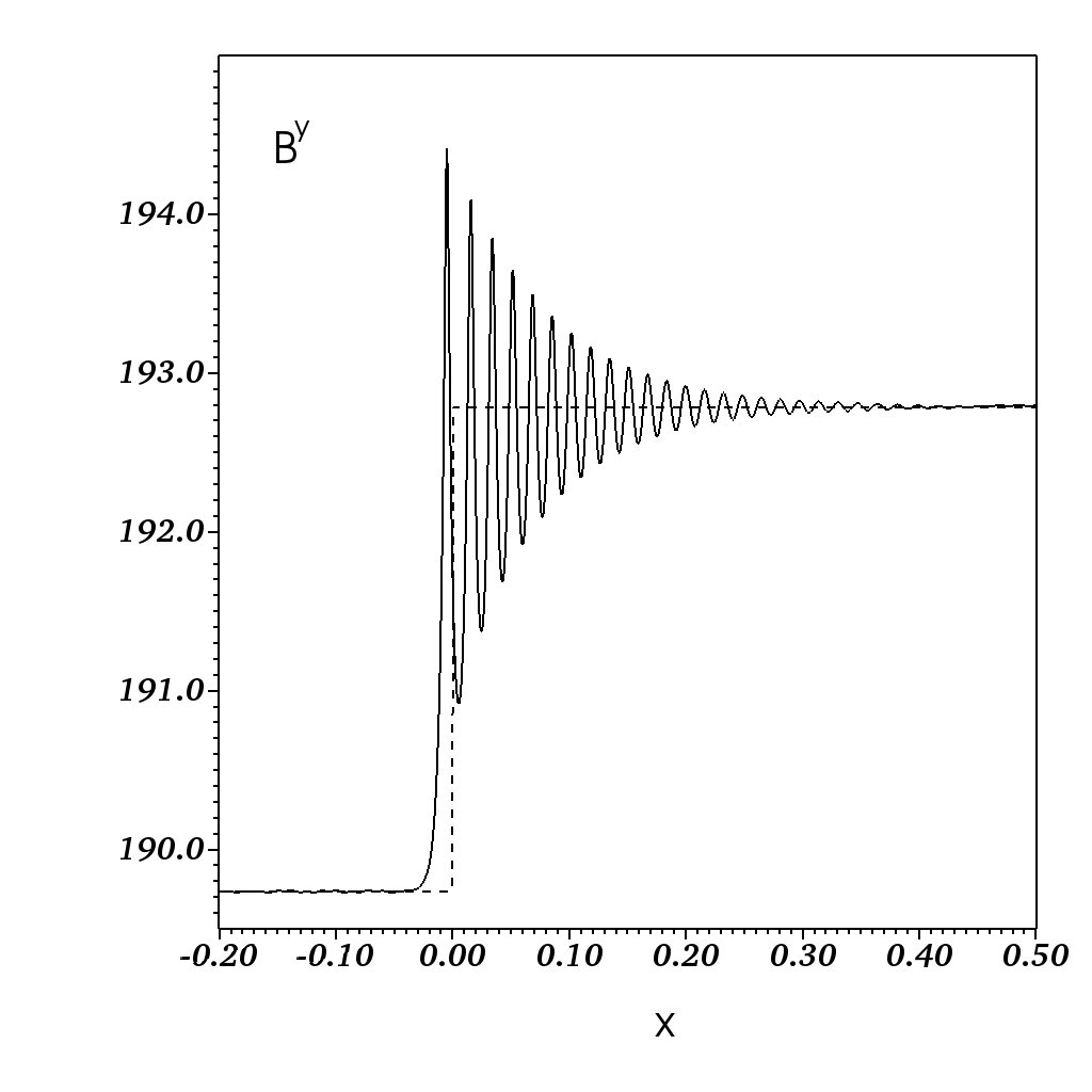
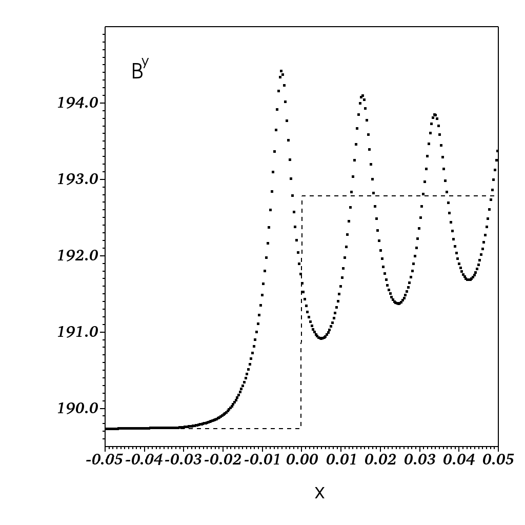
Figure 3: Fast magnetosonic shock case 1. The dashed line shows one-fluid RMHD shock solution. The solid lines in the top panels and the dots in the bottom panels show the numerical two-fluid solution.

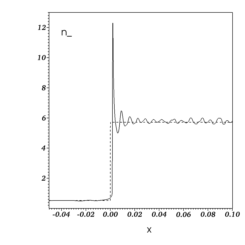
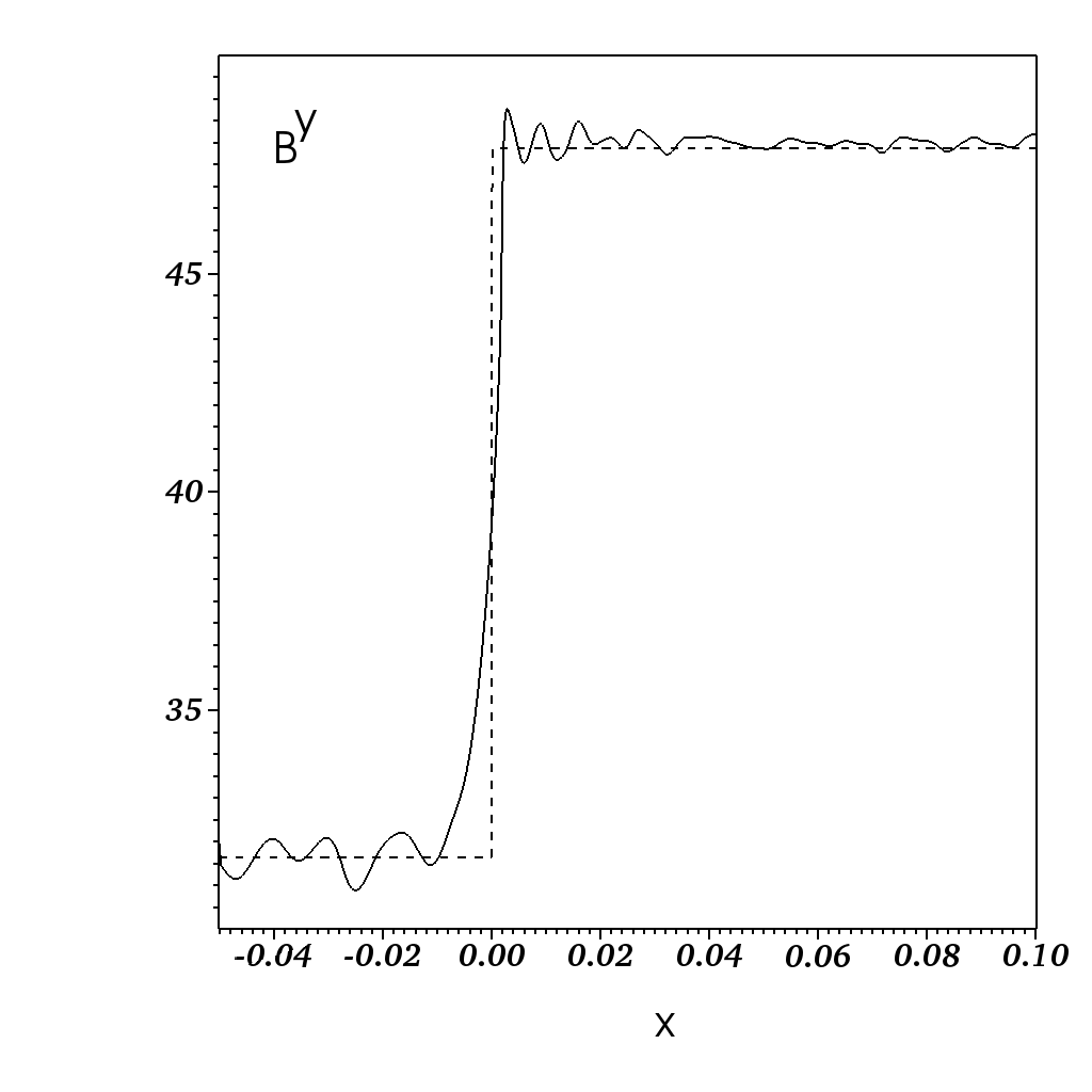
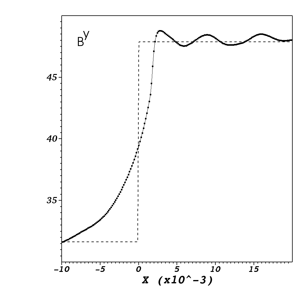
Figure 4: Fast magnetosonic shock case 2. The dashed line shows one-fluid RMHD shock solution. The solid lines in the top panels and the dots in the bottom panels show the numerical two-fluid solution.

Table 3: Perpendicular fast magnetosonic shock solutions used in test simulations. The flow Lorentz factor and magnetic field strength are given in the shock frame.

Case	Left state	Right state
1	$n_{-},n_{+}=0.5$	$n_{-},n_{+}=1.02977$
	$p_{-},p_{+}=0.05$	$p_{-},p_{+}=0.171023$
	$\gamma_{-},\gamma_{+}=10$	$\gamma_{-},\gamma_{+}=4.93331$
	$B=189.728$	$B=192.779$
2	$n_{-},n_{+}=0.5$	$n_{-},n_{+}=5.70015$
	$p_{-},p_{+}=0.05$	$p_{-},p_{+}=8.09570$
	$\gamma_{-},\gamma_{+}=10$	$\gamma_{-},\gamma_{+}=1.32728$
	$B=31.6214$	$B=47.8497$

4.3 Perpendicular fast magnetosonic shocks.

In these tests, we utilized single fluid ideal RMHD solutions for fast magnetosonic shock waves which were obtained by solving the relevant shock equations. Although these solutions are discontinuities the corresponding two-fluid solutions could have continuous structure with or without sub-shocks. In any case, the asymptotic left and right states must be the same as in the single fluid solutions and this explains the virtue of such tests. The sub-shocks may appear as the two-fluid equations do not have terms corresponding to viscosity.

Here we present only the case of perpendicular shock, where the magnetic field is tangent to and the flow velocity is normal to the shock front respectively. The parameters of the one-fluid solutions in the shock frame are given in table 3. They were used to setup discontinuities in the initial data ( Riemann problems ). In both cases, $\mathcal{K}_{\mbox{\scriptsize m}}=\mathcal{K}_{\mbox{\scriptsize f}}=0.01$ and $\mathcal{K}_{\mbox{\scriptsize q}}=0.001$. In the case 1, the numerical grid contained 2000 cells covering the domain $[-0.2,0.5]$, whereas in the case 2, it had 1000 cells and the domain $[-0.05,0.1]$. As to the boundary conditions, we first used the zero gradient ones ( also known as the “free flow” conditions) at both the boundaries, just like in the similar test simulations for our one-fluid RMHD code. However, various waves were emitted from the position of the initial discontinuity in both directions, noticeably upsetting both the boundary states. This resulted in slightly different solutions compared to the reference ones. A somewhat better outcome is obtained when the upstream boundary state is fixed at the reference state. In any case, both boundaries reflect incident waves and the reflected waves interact with the shock, so a certain level of noise is present in the numerical solutions.

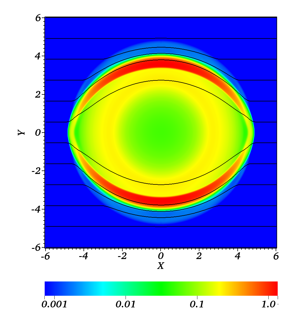
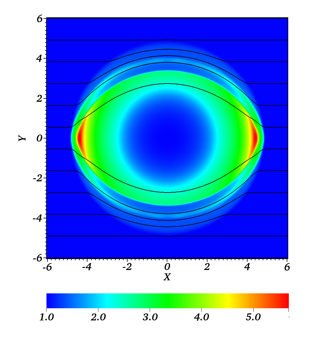
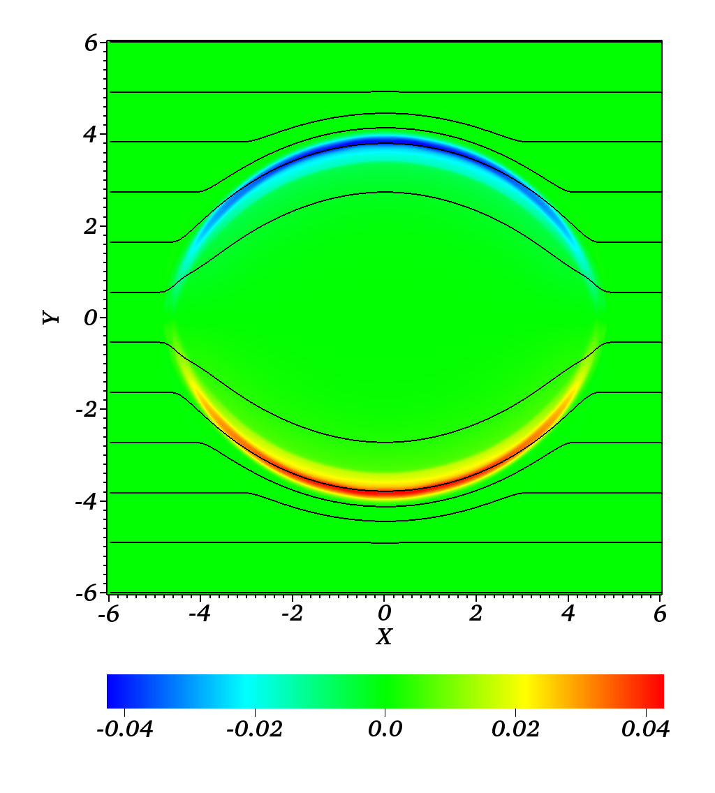
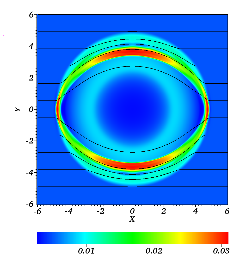
Figure 5: Cylindrical Blast Wave 2D test. Time $t=4$. The top left panel shows the gas pressure, $\log_{10}p_{+}=\log_{10}p_{-}$, The top right panel shows the Lorentz factor $\gamma_{-}=\gamma_{+}$, the maximum value being $\gamma_{\mbox{\scriptsize max}}=5.685$. The bottom left panel shows the z component of electric current, $j^{z}=n_{+}u^{z}_{+}-n_{-}u^{z}_{-}$. The bottom right panel shows the gas density $n_{-}=n_{+}$. All plots show the magnetic field lines.

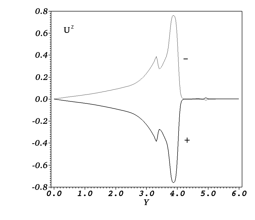
Figure 6: Cylindrical Blast Wave 2D test. Time $t=4$. The solid line shows $u^{z}_{+}$ and the dotted line $u^{z}_{-}$ along the line $x=0$.

Figure 3 shows that in the case 1 the two-fluid solution does not involve a sub-shock – it is continuous in all variables. The downstream part of the solution is a wave-train of gradually diminishing amplitude. The rate of decay is determined by the dimensionless parameter $\mathcal{K}_{\mbox{\scriptsize f}}$, higher $\mathcal{K}_{\mbox{\scriptsize f}}$ yielding slower decay. This suggests that for finite $\mathcal{K}_{\mbox{\scriptsize f}}$, the fixed point of the shock structure equations corresponding to the right state is a stable focus. For $\mathcal{K}_{\mbox{\scriptsize f}}=\infty$, the fixed point must be encircled by a limit cycle. This structure is in general agreement with the analysis of nonrelativistic shocks by Sagdeev (1966). However, the wavelength of the wavetrain is significantly smaller than the skin-depth, which is $\lambda_{\mbox{\scriptsize s}}\simeq 3$, probably due to the relativistic effects. On the contrary, the generalized gyration radius, $R_{g}\simeq 7\times 10^{-4}$, is small compared to the wavelength. When the wavelength is not properly resolved, the numerical solution develops strong oscillations on the cell scale, leading to a crash, unless these oscillations are dumped by high resistivity.

In contrast, the case 2 solution involves a hydro sub-shock – the density, pressure and velocity of the fluids are discontinuous, whereas the electric and magnetic fields are not (see figure 4). Downstream of the sub-shock, one can also see a wave-train similar to that of the case 1 but of smaller amplitude. In both cases, the two-fluid solution agrees with the single fluid solution at $x\to\pm\infty$. In this problem, the generalized gyration radius $R_{g}\simeq 4\times 10^{-3}$ and the skin depth is $\lambda_{\mbox{\scriptsize s}}\simeq 3$.

In our test problems, the flow magnetization $\sigma_{\mbox{\scriptsize m}}\simeq 13$ and $\sigma_{\mbox{\scriptsize m}}\simeq 0.36$ for the cases 1 and 2 respectively. Thus, our results are is in agreement with those of Haim et al. (2012), who analyzed the structure equations of one-dimensional nonlinear perpendicular waves and concluded that continuous soliton-type solutions of two-fluid RMHD do not exist in the low $\sigma_{\mbox{\scriptsize m}}$ limit.

4.4 Cylindrical and Spherical Blast Waves

All the test problems described so far are one-dimensional with the slab symmetry. We used them to test not only our 1D scheme but also the 2D and 3D schemes. In these multi-dimensional tests, the initial solutions were aligned with the grid, so that they varied only along one of the coordinate directions. The disadvantage of such approach is that it excludes waves propagating at an angle to the grid. To verify that the code handles such cases as well, we carried out the following two tests.

The first one is the so-called cylindrical explosion problem, as introduced in Komissarov (1999) for testing ideal RMHD codes and later applied by many other researches. This is a 2D problem with the slab symmetry and it describes the evolution of a cylindrical fireball in a uniform perpendicular magnetic field. The domain is $[-6,6]\times[-6,6]$ with a uniform grid of $400\times 400$ cells. The magnetic field is $B=(1,0,0)$ throughout the domain. The fireball is centered on the origin and its initial radius is $r_{\mbox{\scriptsize b}}=1$. In the surrounding, for $r>r_{\mbox{\scriptsize b}}$, the plasma parameters are $2n_{+}=2n_{-}=0.01$ and $2p_{+}=2p_{-}=0.003$. Initially, inside the fireball $2n_{+}=2n_{-}=1$ and $2p_{+}=2p_{-}=100$ for $r<0.8\,r_{\mbox{\scriptsize b}}$, and these decay exponentially down to the external plasma values for $r_{\mbox{\scriptsize b}}<r<0.8\,r_{\mbox{\scriptsize b}}$ The ratio of specific heats $\Gamma=4/3$. Initially, the velocity vanishes everywhere. $\mathcal{K}_{\mbox{\scriptsize m}}=\mathcal{K}_{\mbox{\scriptsize q}}=0.01$ and $\mathcal{K}_{\mbox{\scriptsize f}}=1$. The dimensionless generalized gyration radius is $R_{\mbox{\scriptsize g}}=0.022$ and $4.0$ outside and inside of the fireball respectively and the corresponding magnetization $\sigma_{\mbox{\scriptsize m}}=23.$ and $1.2\times 10^{-3}$.

Figure 5 illustrates the solution obtained with the 2D code at $t=4$. One can see that angle between the blast wave and the grid varies continuously, covering the whole available range, and so does the angle with the magnetic field. The latter is important as the properties of waves moving along, perpendicular and at an intermediate angle to the magnetic field vary significantly. In ideal MHD, well known degeneracies occur along and perpendicular to the magnetic field. Overall, the two fluid-solution is very similar to the corresponding single fluid ideal (Komissarov, 1999) and resistive (Komissarov, 2007) RMHD solutions, with all the key features present and having similar parameters. The highest Lorentz factor on the grid, $\gamma_{\mbox{\scriptsize max}}=5.685$, is found on the $y=0$ line, very close to the reverse shock. This value is somewhat higher than in the single-fluid solutions. Given the very small size of this high speed region, this difference is most likely to be due to the higher accuracy of the two-fluid simulations (The single fluid codes were only of the second order accuracy.). What is qualitatively different from the single-fluid data is the unequal velocities of the electron and positron fluids. This is illustrated in Figure 6 which shows the z component of the four-velocity along the y axis. It is this difference in velocities which yields the electric current shown in bottom left panel of Figure 5.

This 2D problem was also used to test the 3D code, namely we carried out three test runs with the symmetry axis of the fireball aligned with one of the three basis directions of the 3D Cartesian grid.

The second multi-dimensional test problem deals with a spherical blast wave. The initial setup is the same as in the case of the cylindrical blast wave problem in all respect except the shape of the fireball, which is now a sphere of radius $r_{\mbox{\scriptsize b}}$. The computational domain is $[-4,4]\times[-4,4]\times[-4,4]$ with a uniform grid of $200^{3}$ cells. Figure 7 illustrates the solution at $t=3$. One can see that it is similar to the cylindrical case, with somewhat higher Lorentz factors. There are no features which are grid related and hence artificial in nature.

The results of these tests suggest that multi-fluid codes can be as successful at capturing the large scale dynamics of astrophysical flows as the single-fluid ones.

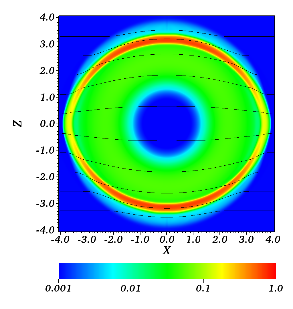
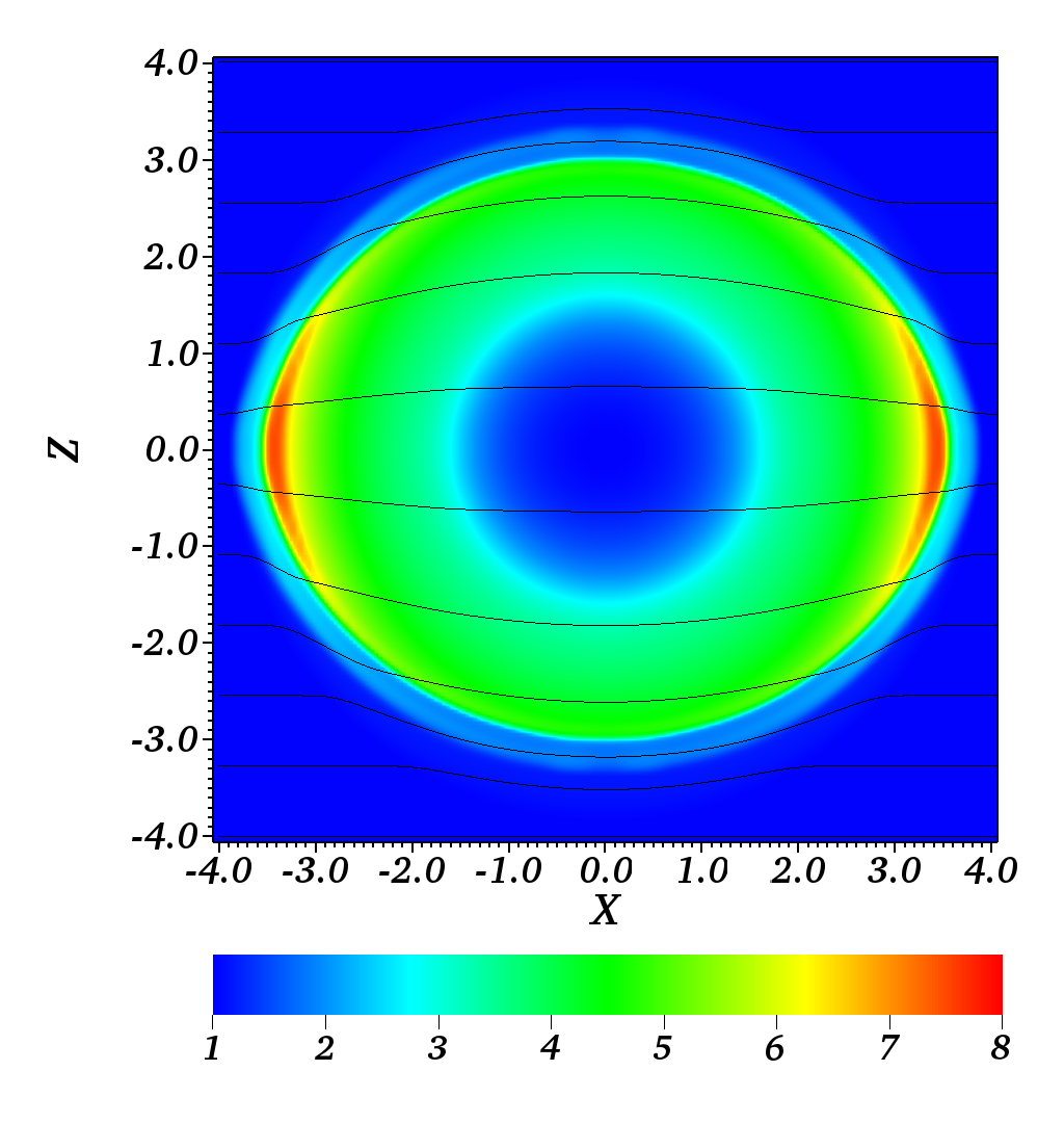
Figure 7: Spherical Blast Wave 3D test. Time $t=3$. The left panel shows the total gas pressure ,$\log_{10}(p_{+}+p_{-})$, and the magnetic field lines in the XOZ plane. The right panel shows the Lorentz factor $\gamma_{-}=\gamma_{+}$, the maximum value being $\gamma_{\mbox{\scriptsize max}}=7.5$.

4.5 Tearing Instability

With the possible exception of the perpendicular shock problems, none of the above simulations test the inter-fluid friction term, which is analogous to resistivity. In the absence of exact analytic solutions of equations with non-vanishing inter-fluid friction term, we are forced simply to try problems where this term is expected to be of critical significance. For example, it is well known that, at least in the single fluid framework, it is the resistivity what drives the tearing instability (e.g. Priest & Forbes, 2000; Lyutikov, 2003; Komissarov et al., 2007). This important problem merits a separate comprehensive study, which we are planning to carry out in the near future. Here we present only the results of two runs for one particular set of parameters.

Following Komissarov et al. (2007) we consider a 2D current sheet with the rotating force-free magnetic field

$$\mn@boldsymbol{B}=B_{0}[\tanh(y/l)\mn@boldsymbol{i}_{x}+\mbox{sech}(y/l)\mn@boldsymbol{i}_{z}]\,,$$ (53)

and a uniform static gas distribution. This configuration is perturbed via modifying the magnetic field, $\mn@boldsymbol{B}\to\mn@boldsymbol{B}+\mn@boldsymbol{b}$, where

$$\mn@boldsymbol{b}=b_{0}\sin(\pi x/\lambda)\mn@boldsymbol{i}_{y}\,.$$ (54)

The computational domain for this simulation is $[-2,+2]\times[-1,+1]$, with the periodic boundary conditions at the x boundaries and the free flow boundary conditions at the y boundaries. The other parameters are $B_{0}=3.0$, $b_{0}=10^{-3}B_{0}$, $\lambda=2$, $l=0.1$, $n_{+}=n_{-}=1$, $p_{+}=p_{-}=0.1$, $\Gamma=4/3$, $\mathcal{K}_{\mbox{\scriptsize m}}=\mathcal{K}_{\mbox{\scriptsize q}}=0.01$ and $\mathcal{K}_{\mbox{\scriptsize f}}=0.3$.

Figure 8: Convergence of the tearing instability solutions. The plots show $\log_{10}B^{y}$ as a function of time for the models with $200\times 200$ ( dashed line ) and $300\times 300$ ( solid line ) cells.

Figure 8 shows the evolution of the maximum value of $B^{y}$ on the grid for two models which differ only by their numerical resolution, one with $200\!\times\!200$ and another with $300\!\times\!300$ cells. One can see the difference between the two solutions is very small, which indicates that the simulations have almost converged. This figure also shows that the perturbation grows approximately exponentially, with gradually decreasing growth rate. At time $t=4$ the e-folding time is $\tau_{e}\simeq 4.3$.

In the approximation of resistive Magnetodynamics this problem was studied in details in Komissarov et al. (2007). In order to compare our growth rate with theirs, we need to scale parameters in the same way. Since in this problem the fluid motion is rather slow, $\gamma_{\pm}<1.008$, the resistivity is accurately represented by the expression

$$\eta\simeq\frac{c^{2}\varkappa_{\mbox{\scriptsize f}}}{4\pi e^{2}}$$ (55)

(see Eq.14). The corresponding dimensionless resistivity is

$$\eta\simeq\frac{\mathcal{K}_{\mbox{\scriptsize m}}\mathcal{K}_{\mbox{\scriptsize q}}}{\mathcal{K}_{\mbox{\scriptsize f}}}\simeq 3.3\times 10^{-4}\,$$ (56)

and hence the resistive time-scale of the current sheet

$$\tau_{d}=l^{2}/\eta\simeq 30\,.$$

The dimensionless Alfvén speed

$$v_{\mbox{\scriptsize a}}^{2}=\frac{B^{2}}{B^{2}+(\mathcal{K}_{\mbox{\scriptsize m}}/\mathcal{K}_{\mbox{\scriptsize q}})(w_{+}+w_{-})}\simeq 0.76\,,$$

leading to the Alfvén time-scale

$$\tau_{a}=l/v_{\mbox{\scriptsize a}}\simeq 0.11$$

and the Lundquist number

$$\mbox{Lu}=\sqrt{2}\frac{\tau_{\mbox{\scriptsize d}}}{\tau_{\mbox{\scriptsize a}}}\sim 370\,.$$

Komissarov et al. (2007) have shown that in the limit of Magnetodynamics, the growth rate of perturbations peaks at $k^{*}\simeq\mbox{Lu}^{-1/4}l^{-1}$ and the shortest e-folding time scales as

$$\tau_{\mbox{\scriptsize e}}\propto(\tau_{\mbox{\scriptsize d}}\tau_{\mbox{\scriptsize a}})^{1/2}\,.$$ (57)

In fact, their simulations show that for Lu=140 the coefficient of proportionality is $\simeq 1.8$. In our test simulations $k\simeq 1.4k^{*}$ and the coefficient $\simeq 2.3$. Thus, our results are very close to their findings.

The left panels of Figure 9 demonstrate how the instability leads to tearing of the current sheet during the non-linear phase. Its right panels show in more details the structure of the higher resolution solution by the end of the simulation, at $t=30$. The solution exhibits expected features, such as the sub-layer of strong electric current, magnetic islands etc.

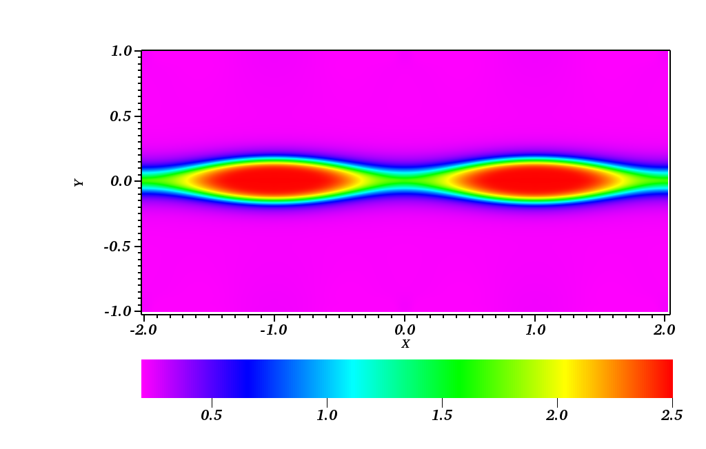
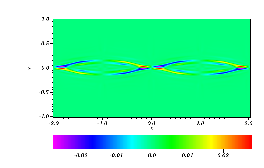
Figure 9: Tearing instability 2D test. The left panels show the $B^{z}$ component of the magnetic field at times $t=0$, 15 and 30, from top to bottom. The right panels show $p_{\mbox{\scriptsize mat}}=p_{-}+p_{+}$ ( top ), $j^{z}=n_{+}u^{z}_{+}-n_{-}u^{z}_{-}$ ( middle ) and $q=n_{+}\gamma_{+}-n_{-}\gamma_{-}$ ( bottom ) at $t=30$.

5 Conclusion

In this paper we considered the equations of relativistic two-fluid Magnetohydrodynamics for electron-positron plasma and described a high-order explicit finite-difference scheme for their numerical integration. This work was carried out as a part of the search for the most adequate mathematical model for the macroscopic dynamics of relativistic magnetized plasma, with astrophysical applications in mind. There are reasons to believe that this model has advantages compared to both ideal and resistive RMHD. Indeed, the ideal RMHD assumes $\mn@boldsymbol{E}\!\cdot\!\mn@boldsymbol{B}=0$ and $E^{2}<B^{2}$ and hence allows magnetic dissipation only by slow shocks. The resistive RMHD allows resistive magnetic dissipation but utilizes a simplistic phenomenological Ohm’s law. Both do not capture plasma waves above the plasma frequency. The two-fluid approach allows more realistic Ohm’s law via introduction of some microphysics into the system. Yet, it seems to remain oriented more towards the large-scale (macroscopic) dynamics. While other frameworks, like particle dynamics and kinetic models, capture the plasma microphysics much better, they are not practical for simulating phenomena with characteristic length scales greatly exceeding the gyration radius. Our scheme will help to explore the practicality of the two-fluid framework.

The scheme integrates dimensionless equations which include three parameters, $\mathcal{K}_{\mbox{\scriptsize m}}$, $\mathcal{K}_{\mbox{\scriptsize q}}$, and $\mathcal{K}_{\mbox{\scriptsize f}}$, introduced by analogy with the Reynolds number. In some applications, they may be of order unity. In others, much lower or much higher than unity. Our numerical scheme has its limitations and will not always be able to cope with extreme values. However, if the solution reaches asymptotic regimes rapidly it may not be necessary to deal with such extremes. Systematic studies of the parameter space will be required to establish if this is the case.

The design of our numerical scheme is based on standard modern techniques developed for systems of hyperbolic conservation laws. In particular, we use third-order WENO interpolation to setup Riemann problems at the cell interfaces, the hyperbolic fluxes are computed using the Lax-Friedrich formula and the explicit time integration is carried out with third order TVD Runge-Kutta scheme. The results of test simulations presented in Sec.4 show that the numerical scheme is sufficiently robust and confirm its third-order accuracy.

The test simulations revealed that in some problems including strong shocks the two-fluid shock structure may have oscillations on the length scale below the skin depth. When not fully resolved, these are problematic and can lead to code crashing. However, they can be damped with high localized resistivity. A more serious limitation concerns the plasma magnetization. Similarly to the existing explicit conservative schemes for single fluid RMHD, this scheme fails when $\sigma_{\mbox{\scriptsize m}}\gg 1$. The reason for this is the very large magnetic terms compared to the gas ones in Eqs.25,26. Equivalently, the source terms in Eqs.16,17 corresponding to the Lorentz force become very stiff in this limit. A different approach will be required to overcome this limitation. One possible solution is an IMEX (implicit-explicit) type of scheme (e.g. Kumar & Misra, 2012).

Here we considered only the case of electron-positron plasma. Although, this is already of significant interest in many astrophysical problems, in other applications, protons and even neutrons need to be included. This is another potential direction for continuation of this work.

The current version of our code, named JANUS, can be provided by the authors on request.

6 Acknowledgments

The authors would like to thank Anatoly Spitkovsky and Michael Gedalin for helpful discussions and the anonymous referee for useful comments. SSK acknowledges support by STFC under the standard grant ST/I001816/1. VK, AZ and SSK acknowledge support from the Russian Ministry of Education and Research under the state contract 14.B37.21.0915 for Federal Target-Oriented Program. BMV acknowledges partial support by RFBR grant 12-02-01336-a.

References

- Akhiezer & Polovin (1956) Akhiezer A. I., Polovin R. V., 1956, Sov.Phys.-JETP, 3, 696
- Amano & Kirk (2013) Amano T., Kirk J. G., 2013, ApJ, 770, 18
- Arons et al. (2005) Arons J., Backer D. C., Spitkovsky A., Kaspi V. M., 2005, in Rasio F. A., Stairs I. H., eds, Binary Radio Pulsars Vol. 328 of Astronomical Society of the Pacific Conference Series, Probing Relativistic Winds: The Case of PSR J0737-3039 A and B. p. 95
- Dedner et al. (2002) Dedner A., Kemm F., Kröner D., Munz C.-D., Schnitzer T., Wesenberg M., 2002, J.Comp.Phys., 175, 645
- Falle & Komissarov (1996) Falle S. A. E. G., Komissarov S. S., 1996, MNRAS, 278, 586
- Goedbloed & Poedts (2004) Goedbloed J. P. H., Poedts S., 2004, Principles of Magnetohydrodynamics
- Gurovich & Solov’ev (1986) Gurovich V. T., Solov’ev L. S., 1986, JETP, 91, 1144
- Haim et al. (2012) Haim L., Gedalin M., Spitkovsky A., Krasnoselskikh V., Balikhin M., 2012, Journal of Plasma Physics, 78, 295
- Kojima & Oogi (2009) Kojima Y., Oogi J., 2009, MNRAS, 398, 271
- Komissarov (1999) Komissarov S. S., 1999, MNRAS, 303, 343
- Komissarov (2007) Komissarov S. S., 2007, MNRAS, 382, 995
- Komissarov et al. (2007) Komissarov S. S., Barkov M., Lyutikov M., 2007, MNRAS, 374, 415
- Kumar & Misra (2012) Kumar H., Misra S., 2012, Journal of Scientific Computing, 52, 401
- Liu et al. (1994) Liu X.-D., Osher S., Chan T., 1994, J.Comp.Phys., 115, 200
- Lyutikov (2003) Lyutikov M., 2003, MNRAS, 346, 540
- Max (1973) Max C. E., 1973, Physics of Fluids, 16, 1277
- Munz et al. (2000) Munz C.-D., Omnes P., Schneider R., Sonnendrücker E., Voß U., 2000, J.Comp.Phys., 161, 484
- Priest & Forbes (2000) Priest E., Forbes T., 2000, Magnetic Reconnection
- Sagdeev (1966) Sagdeev R. Z., 1966, Reviews of Plasma Physics, 4, 23
- Sakai & Kawata (1980) Sakai J., Kawata T., 1980, Journal of the Physical Society of Japan, 49, 747
- Shu & Osher (1988) Shu C.-W., Osher S., 1988, J.Comp.Phys., 77, 439
- Spitkovsky & Arons (2002) Spitkovsky A., Arons J., 2002, in Slane P. O., Gaensler B. M., eds, Neutron Stars in Supernova Remnants Vol. 271 of Astronomical Society of the Pacific Conference Series, Simulations of Pulsar Wind Formation. p. 81
- Yamaleev & Carpenter (2009) Yamaleev N. K., Carpenter M. H., 2009, J.Comp.Phys., 228, 3025
- Zenitani et al. (2009a) Zenitani S., Hesse M., Klimas A., 2009a, ApJ, 705, 907
- Zenitani et al. (2009b) Zenitani S., Hesse M., Klimas A., 2009b, ApJ, 696, 1385