Diffusive Molecular Communication with Disruptive Flows

Abstract

In this paper, we study the performance of detectors in a diffusive molecular communication environment where steady uniform flow is present. We derive the expected number of information molecules to be observed in a passive spherical receiver, and determine the impact of flow on the assumption that the concentration of molecules throughout the receiver is uniform. Simulation results show the impact of advection on detector performance as a function of the flow’s magnitude and direction. We highlight that there are disruptive flows, i.e., flows that are not in the direction of information transmission, that lead to an improvement in detector performance as long as the disruptive flow does not dominate diffusion and sufficient samples are taken.

I Introduction

Future applications of nanotechnology will be enabled by the ability of individual devices with nanoscale components to communicate amongst themselves and share information. Fields that require diagnostics or actions on a small scale, such as healthcare and manufacturing, are envisioned to benefit from the deployment of these connected devices, collectively known as nanonetworks; see [1, 2]. Molecular communication is a physical layer design strategy for nanonetworks where transmitters release molecules that freely travel or are carried to their intended destinations. This strategy is bio-inspired; cellular systems use molecules to communicate via integration with biochemical mechanisms; see [3].

The simplest molecular transport mechanism is free diffusion, where molecules move randomly due to collisions with other molecules in the environment. No external energy is required, unlike in active propagation methods where energy is consumed to direct molecules towards the receiver. Furthermore, networks of devices communicating via diffusion can form spontaneously because there are no fixed connections between devices. However, communication via diffusion alone is limited by both propagation time and reliability as the distance between devices increases. In a purely diffusive environment, intersymbol interference (ISI) is a major problem because the receiver cannot differentiate between the arrivals of the same type of molecule emitted at different times.

Flows play an important role in many diffusive environments where molecular communication networks may be deployed, especially when the distance that molecules must travel is greater than what can be practically achieved via diffusion alone. For example, the advection of blood in the body enables the transport of oxygen from the lungs to tissues and also facilitates the removal of waste and toxic molecules via the liver and kidneys; see [3]. Flows can also help mitigate ISI in a communications context by carrying “old” molecules away from the receiver.

Analytically, the simplest flow is both steady and uniform. In a steady flow, the pressure, density, and velocity components at each point in the stream do not change with time; see [4]. If uniform, then these components are identical throughout the environment of interest. Existing literature in molecular communication has generally assumed that flow is not only both steady and uniform (which are not necessarily realistic assumptions), but also only in the direction of transmission, i.e., in the same direction as a line pointing from the transmitter to its intended receiver, cf. e.g. [5, 6, 7]. We define disruptive flows as any flow component that is not in the direction of transmission. These flows are literally destructive in that they reduce the peak number of molecules expected to be observed at the receiver.

In [8], we studied receiver detection schemes for a 3-dimensional stochastic diffusion environment between a single transmitter and receiver. Our physical model included steady uniform flow in any direction (a notion that was also recently considered in a 2-dimensional environment in [9]). Simulation results showed the average detector bit error probabilities under a few sample cases of flow. We observed that there were disruptive flows under which both optimal and suboptimal detectors could improve over the no-flow case, because the advective removal of unintended (ISI) molecules mitigated the removal of intended molecules. These results suggested that bi-directional transmission in flowing environments is not only possible but could actually be better than in an environment without flow. Thus, it is of interest to investigate precisely under what conditions advection is beneficial to diffusive communication, i.e., what magnitudes and directions of flow decrease the probability of bit errors for which detectors, and when advection degrades communication.

Furthermore, we assumed for tractability of analysis in [8] that the expected concentration of information molecules throughout the receiver was equal to that expected at the center of the receiver. We hereafter refer to this assumption as the uniform concentration assumption. We assessed this assumption’s accuracy in environments without flow in [10], but evaluating its accuracy in flowing environments has been an open problem.

This paper extends the consideration of steady uniform flow in [8] to make the following contributions:

1. We derive the expected number of information molecules at an ideal spherical receiver due to an emission by a point source into an unbounded diffusive environment with a steady uniform flow. The derivation is made without the uniform concentration assumption and a closed-form solution is possible only when the flow is parallel to a line joining the source and receiver.

2. We assess the uniform concentration assumption by measuring the relative deviation in the expected concentration of information molecules when the assumption is applied. This comparison is made using dimensionless values, as we used in [10], so that the results scale to any reference dimension.

3. We compare the performance of the optimal and weighted sum detectors described in [8] under a wide range of steady uniform flows. We discuss the types of flow for which detector performance is improved over the no-flow case, highlighting disruptive flows that enable a decrease in the probability of error.

We note that, in [8], we also considered the presence of enzyme molecules in the propagation environment that are capable of degrading the information molecules as a strategy to mitigate ISI. For clarity of exposition, and because advection can also mitigate ISI, we do not include the effect of enzymes in the model presented in this paper. However, all results presented here can be easily extended to the case where enzymes are in the propagation environment.

The rest of this paper is organized as follows. The physical environment is described in dimensional and dimensionless forms and the detectors are summarized in Section II. In Section III, we derive the expected number of molecules observed at the receiver, both with and without the uniform concentration assumption. In Section IV, we summarize the optimal and weighted sum detectors that we presented in [8]. Numerical and simulation results are presented in Section V. We draw our conclusions in Section VI.

II System Model

In this section, we describe the system model that we considered in [8] and then, unlike in [8], translate it into dimensionless form.

II-A Dimensional Form

The receiver is a sphere with radius $r_{obs}$ and volume $V_{obs}$ that is fixed and centered at the origin of an infinite, 3-dimensional aqueous environment of constant uniform temperature and viscosity. The transmitter is fixed at location $\{-x_{0},0,0\}$ (without loss of generality). By symmetry, the concentrations observed in this environment are equivalent (by a factor of 2) to those in the semi-infinite case where $z\geq 0$ is the aqueous environment, the $xy$-plane is an elastic boundary, and the receiver is a hemisphere whose circle face lies on the boundary; see [11, Eq. 2.7]. This equivalent environment could describe, for example, a small transmitter and receiver mounted along the wall of a large blood vessel or artery. The receiver is a (virtual) passive observer that does not impede diffusion or initiate chemical reactions (this assumption focuses our analysis on the impact of the propagation environment and enables tractability). A steady uniform flow (or drift) exists and is defined by its velocity component along each dimension, i.e., $\vec{v}=\{v_{x},v_{y},v_{z}\}$. The placement of the transmitter is so that a positive $v_{x}$ is in the direction of the receiver from the transmitter. Thus, a negative $v_{x}$, a nonzero $v_{y}$, or a nonzero $v_{z}$ represent disruptive flows.

The transmitter has a binary sequence of length $B$, $\mathbf{W}=\{W\left[1\right],W\left[2\right],\dots,W\left[B\right]\}$, to send to the receiver, where $W\left[j\right]$ is the $j$th information bit and $\Pr(W\left[j\right]=1)=P_{1}$. The transmitter uses binary modulation and transmission intervals of duration $T_{int}$ seconds. To send a binary $1$, $N_{EM}$ $A$ molecules are released at the start of the bit interval. To send a binary $0$, no molecules are released.

We assume that the environment has additional sources of $A$ molecules, for example via interference from other communication links or via some other chemical process that generates $A$ molecules. These external noise sources are distinct from the diffusion of $A$ molecules emitted by the transmitter. As in [8], we only assume that we know the cumulative impact of all noise sources on the received signal, and that we can characterize this impact as a Poisson random variable with time-varying mean $\overline{{N_{A}}_{n}}\left(t\right)$. This noise model is sufficient to model either of the example cases above. However, we omit the impact of steady uniform flow on the noise sources themselves (since we do not specify the origin of the noise), and we will only consider additive noise sources with constant mean in our simulations. We leave a more precise characterization of noise and interference for future work.

The concentration of $A$ molecules at the point defined by vector $\vec{r}$ and at time $t$ in $\textnormal{molecule}\cdot\textnormal{m}^{-3}$ is $C_{A}(\vec{r},t)$ (or written as $C_{A}$ for compactness). We assume that these molecules diffuse independently once they are released by the transmitter or noise sources. In addition, due to the constant uniform temperature and viscosity of the environment, the $A$ molecules diffuse with constant diffusion coefficient $D_{A}$. The differential equation describing the motion of $A$ molecules due to both diffusion and advection is a modified version of Fick’s second law, written as [12, Ch. 4]

$$\frac{\partial C_{A}}{\partial t}=D_{A}\nabla^{2}C_{A}-v_{x}\frac{\partial C_{A}}{\partial x}-v_{y}\frac{\partial C_{A}}{\partial y}-v_{z}\frac{\partial C_{A}}{\partial z},$$ (1)

which can be easily solved to find the expected point concentration due to an emission of $N_{EM}$ molecules by the transmitter at time $t=0$. It is easy to show with a moving reference frame that this expected concentration at point $\{x,y,z\}$ is

$$C_{A}=\frac{N_{EM}}{(4\pi D_{A}t)^{3/2}}\exp\left(-\frac{|\vec{r}|^{2}}{4D_{A}t}\right),$$ (2)

where $|\vec{r}|^{2}=(x+x_{0}-v_{x}t)^{2}+(y-v_{y}t)^{2}+(z-v_{z}t)^{2}$ is the square of the effective distance from the transmitter at $\{-x_{0},0,0\}$ to $\{x,y,z\}$.

II-B Dimensionless Form

For dimensional analysis, reference variables are used to scale all parameters into dimensionless form; please refer to [13] for more on dimensional analysis. As in [10], we define reference distance $L$ in m and reference number of molecules $N_{EM}$ (i.e., the transmitter releases one dimenionless molecule to send a binary $1$). We also define reference concentration $C_{0}=N_{EM}/L^{3}$ in $\textnormal{molecule}\cdot\textnormal{m}^{-3}$. We then define the dimensionless concentration of $A$ molecules as $C_{a}^{\star}=C_{A}/C_{0}$, dimensionless time as $t^{\star}=D_{A}t/L^{2}$, and dimensionless coordinates along the three axes as

$$x^{\star}=\frac{x}{L},\quad y^{\star}=\frac{y}{L},\quad z^{\star}=\frac{z}{L},$$ (3)

such that variables with a “$\star$” superscript are equal to the corresponding dimensional variables scaled by the appropriate reference variables. Advection is represented dimensionlessly with the Peclet number, $v^{\star}$, written as [3, Eq. 1.3.1]

$$v^{\star}=\frac{vL}{D_{A}},$$ (4)

where $v=|\vec{v}|$ is the speed of the fluid. $v^{\star}$ measures the relative impact of advection versus diffusion on molecular transport. If $v^{\star}\ll 1$, i.e., if $v\to 0$, then diffusion dominates particle motion and advection can be ignored. If $v^{\star}\gg 1$, then advection dominates particle motion and diffusion can be ignored. Under advection-dominant motion, disruptive flows should prevent successful communication (no matter what detector is used) and non-disruptive flows should aid communication (as long as the receiver takes a sample while molecules are flowing through it). Thus, the impact of steady uniform flow on communication depends on the direction of flow, and it is important to consider $v^{\star}$-values much less and much greater than $1$. We define $v^{\star}$ along each dimension as

$$v^{\star}_{\scriptscriptstyle\parallel}=\frac{v_{x}L}{D_{A}},\quad v^{\star}_{\perp,1}=\frac{v_{y}L}{D_{A}},\quad v^{\star}_{\perp,2}=\frac{v_{z}L}{D_{A}},$$ (5)

but we note that, without loss of generality (because the transmitter is on the $x$-axis), we can set $v^{\star}_{\perp,2}=0$ and write $v^{\star}_{\perp,1}=v^{\star}_{\perp}$. Given the dimensionless model, (1) becomes

$$\frac{\partial C_{a}^{\star}}{\partial t^{\star}}=\nabla^{2}C_{a}^{\star}-v^{\star}_{\scriptscriptstyle\parallel}\frac{\partial C_{a}^{\star}}{\partial x^{\star}}-v^{\star}_{\perp}\frac{\partial C_{a}^{\star}}{\partial y^{\star}},$$ (6)

where

$$\frac{\partial C_{a}^{\star}}{\partial t^{\star}}= \;\frac{\partial C_{A}}{\partial t}\frac{L^{2}}{D_{A}C_{0}},\quad\nabla^{2}C_{a}^{\star}=\frac{L^{2}}{C_{0}}\nabla^{2}C_{A},$$ (7)

$$\frac{\partial C_{a}^{\star}}{\partial x^{\star}}= \;\frac{\partial C_{A}}{\partial x}\frac{L}{C_{0}},\quad\frac{\partial C_{a}^{\star}}{\partial y^{\star}}=\frac{\partial C_{A}}{\partial y}\frac{L}{C_{0}},$$ (8)

and (2) becomes

$$C_{a}^{\star}=\frac{1}{(4\pi t^{\star})^{3/2}}\exp\left(\frac{-|\vec{r}^{\star}|^{2}}{4t^{\star}}\right),$$ (9)

where $|\vec{r}^{\star}|^{2}=(x^{\star}+x^{\star}_{0}-v^{\star}_{\scriptscriptstyle\parallel}t^{\star})^{2}+(y^{\star}-v^{\star}_{\perp}t^{\star})^{2}+{z^{\star}}^{2}$ is the square of the effective distance from the transmitter at $\{-x^{\star}_{0},0,0\}$ to $\{x^{\star},y^{\star},z^{\star}\}$.

III Receiver Signal

In this section, we derive the expected dimensionless number of molecules observed at the receiver that were emitted by the transmitter at $t^{\star}=0$, $\overline{{N_{a}}_{0}^{\star}}\left(t^{\star}\right)$. This derivation enables comparison with the uniform concentration assumption, i.e., the assumption that the expected concentration of information molecules throughout the receiver is equal to that expected at the center of the receiver. Then, we write the general time-varying receiver signal ${N_{A}}_{obs}\!\left(t\right)$ as a function of the transmitter’s emissions and the external noise sources.

The receiver is a passive observer, so the expected dimensionless number of $A$ molecules within the dimensionless receiver volume is found by integrating (9) over $V_{obs}^{\star}$, i.e.,

$$\overline{{N_{a}}_{0}^{\star}}\left(t^{\star}\right)=\int\limits_{0}^{r_{obs}^{\star}}\int\limits_{0}^{2\pi}\int\limits_{0}^{\pi}C_{a}^{\star}{r_{i}^{\star}}^{2}\sin\theta d\theta d\phi dr_{i}^{\star},$$ (10)

where $r_{i}^{\star}$ is the magnitude of the distance from the origin (i.e., the center of the receiver) to the arbitrary point $\{x^{\star},y^{\star},z^{\star}\}$ within $V_{obs}^{\star}$. The first step in solving (10) is to convert $|\vec{r}^{\star}|^{2}$ in (9) from Cartesian to spherical coordinates. It is straightforward to show that

$$|\vec{r}^{\star}|^{2}= \;{r_{i}^{\star}}^{2}+{x^{\star}_{0}}^{2}-2t^{\star}x^{\star}_{0}v^{\star}_{\scriptscriptstyle\parallel}-2x^{\star}_{0}r_{i}^{\star}\cos\phi\sin\theta$$

$$-2t^{\star}r_{i}^{\star}\left(v^{\star}_{\scriptscriptstyle\parallel}\cos\phi\sin\theta+v^{\star}_{\perp}\sin\phi\sin\theta\right)$$

$$+{t^{\star}}^{2}\left({v^{\star}_{\scriptscriptstyle\parallel}}^{2}+{v^{\star}_{\perp}}^{2}\right),$$ (11)

where $\phi=\tan^{-1}\left(y^{\star}/x^{\star}\right)$ and $\theta=\cos^{-1}\left(z^{\star}/r_{i}^{\star}\right)$. Generally, (10) does not have a known closed-form solution, due to the sum of trigonometric terms in the exponential in (9). We can integrate (10) over $r_{i}^{\star}$ using substitution, integration by parts, the definition of the error function, i.e., [14, Eq. 3.1.1]

$$\operatorname{erf}\left(a\right)=\frac{2}{\pi^{\frac{1}{2}}}\int_{0}^{a}\exp\left(-b^{2}\right)db,$$ (12)

and the integral [14, Eq. 4.1.4]

$$\int a\operatorname{erf}\left(a\right)da=\frac{1}{2}\operatorname{erf}\left(a\right)\left(a^{2}-\frac{1}{2}\right)+\frac{a}{2\pi^{\frac{1}{2}}}\exp\left(-a^{2}\right).$$ (13)

It can then be shown that $\overline{{N_{a}}_{0}^{\star}}\left(t^{\star}\right)$ becomes the integration of

$$(2\pi^{\frac{3}{2}})^{-1}\exp\left(\beta_{1}^{2}t^{\star}+\beta_{2}\right)\sin\theta\Big{[}\beta_{1}{t^{\star}}^{\frac{1}{2}}\exp\left(-\beta_{1}^{2}{t^{\star}}\right)+\pi^{\frac{1}{2}}/2$$

$$\times\left(1+2\beta_{1}^{2}{t^{\star}}\right)\!\!\left(\operatorname{erf}\left(r_{obs}^{\star}{t^{\star}}^{-\frac{1}{2}}/2-\beta_{1}{t^{\star}}^{\frac{1}{2}}\right)\!-\operatorname{erf}\left(-\beta_{1}{t^{\star}}^{\frac{1}{2}}\right)\right)$$

$$-\left(\beta_{1}{t^{\star}}^{\frac{1}{2}}+r_{obs}^{\star}{t^{\star}}^{-\frac{1}{2}}/2\right)\exp\left(-(r_{obs}^{\star}{t^{\star}}^{-\frac{1}{2}}/2-\beta_{1}{t^{\star}}^{\frac{1}{2}})^{2}\right)\Big{]},$$ (14)

over $\theta\in[0,\pi]$ and $\phi\in[0,2\pi]$, where

$$\beta_{1}= \;\frac{\sin\theta}{2}\left(v^{\star}_{\scriptscriptstyle\parallel}\cos\phi+v^{\star}_{\perp}\sin\phi+\frac{x^{\star}_{0}}{t^{\star}}\cos\phi\right),$$ (15)

$$\beta_{2}= \;\frac{x^{\star}_{0}v^{\star}_{\scriptscriptstyle\parallel}}{2}-\frac{t^{\star}}{4}\left({v^{\star}_{\scriptscriptstyle\parallel}}^{2}+{v^{\star}_{\perp}}^{2}\right)-\frac{{x^{\star}_{0}}^{2}}{4t^{\star}}.$$ (16)

For general steady uniform flow $v^{\star}\neq 0$, (10) can be solved by numerically integrating (14) over $\theta$ and $\phi$. However, for the special case $v^{\star}_{\perp}=0$, such that the direction of flow is parallel to a line between the source and receiver, we can apply Theorem 2 in [10] using a change of variables and solve (10) as

$$\overline{{N_{a}}_{0}^{\star}}\left(t^{\star}\right)= \;\frac{1}{2}\left[\operatorname{erf}\left(\frac{r_{obs}^{\star}\!-\vec{r}_{eff}^{\star}}{2{t^{\star}}^{\frac{1}{2}}}\right)+\operatorname{erf}\left(\frac{r_{obs}^{\star}\!+\vec{r}_{eff}^{\star}}{2{t^{\star}}^{\frac{1}{2}}}\right)\right]$$

$$+\frac{1}{\vec{r}_{eff}^{\star}}\sqrt{\frac{t^{\star}}{\pi}}\Bigg{[}\exp\left(-\frac{(\vec{r}_{eff}^{\star}+r_{obs}^{\star})^{2}}{4t^{\star}}\right)$$

$$-\exp\left(-\frac{(\vec{r}_{eff}^{\star}-r_{obs}^{\star})^{2}}{4t^{\star}}\right)\Bigg{]},$$ (17)

where $\vec{r}_{eff}^{\star}=-\left(x^{\star}_{0}-v^{\star}_{\scriptscriptstyle\parallel}t^{\star}\right)$ is the effective distance along the $x^{\star}$-axis from the transmitter to the center of the receiver.

If we apply the uniform concentration assumption, then the evaluation of (10) is simply the product of $V_{obs}^{\star}$ and $C_{a}^{\star}$ at the center of the receiver, i.e., at the origin. Thus, we have

$$\overline{{N_{a}}_{0}^{\star}}\left(t^{\star}\right)=\frac{V_{obs}^{\star}}{(4\pi t^{\star})^{3/2}}\exp\left(-\frac{{\vec{r}_{eff}^{\star}}{}^{2}}{4t^{\star}}-\frac{{t^{\star}}{v^{\star}_{\perp}}^{2}}{4}\right),$$ (18)

and in Section V we will measure the relative deviation of (18) from (10), where (10) is solved using (17) if $v^{\star}_{\perp}=0$ and by numerically integrating (14) otherwise.

It is straightforward to derive the statistics of the general receiver signal ${N_{A}}_{obs}\!\left(t\right)$ based on $\overline{{N_{a}}_{0}^{\star}}\left(t^{\star}\right)$ and the transmitter sequence $\mathbf{W}$. Assuming constant ideal diffusion, then the behavior of individual $A$ molecules is independent, and ${N_{A}}_{obs}\!\left(t\right)$ is a sum of time-varying Poisson random variables (as described in [8]), with time-varying mean

$$\overline{{N_{A}}_{obs}}(t)=\overline{{N_{A}}_{TX}}\left(t\right)+\overline{{N_{A}}_{n}}\left(t\right),$$ (19)

where $\overline{{N_{A}}_{n}}\left(t\right)$ is the mean number of molecules from the noise sources, $\overline{{N_{A}}_{TX}}\left(t\right)$ is the mean number of molecules from emissions by the transmitter, i.e.,

$$\overline{{N_{A}}_{TX}}\left(t\right)=\sum_{j=1}^{\lfloor\frac{t}{T_{int}}+1\rfloor}W\left[j\right]\overline{{N_{A}}_{0}}\left(t-(j-1)T_{int}\right),$$ (20)

and $\overline{{N_{A}}_{0}}\left(t\right)$ is $\overline{{N_{a}}_{0}^{\star}}\left(t^{\star}\right)$ in dimensional form.

IV Detector Summary

To study the impact of advection on detector performance, we implement the detectors that we proposed in [8]. In this section, we summarize these detectors. The detectors rely on a common sampling scheme, where the receiver makes $M$ observations in every bit interval, and we assume in this paper that the observations are independent. The value of the $m$th observation in the $j$th interval is labeled $s_{j,m}$. We define the sampling times within a single interval as the function $g\left(m\right)$, and the global time sampling function $t\left(j,m\right)=jT_{int}+g\left(m\right)$, where $j=\{1,2,\ldots,B\},m=\{1,2,\ldots,M\}$. We assume that the transmitter and receiver are perfectly synchronized. Synchronization amongst devices in a non-advective environment was achieved in [15] via the diffusion of inhibitory molecules. However, synchronization in flowing environments remains an open problem.

We use the maximum likelihood optimal sequence detector to give a lower bound on the bit error probability. The optimal receiver decision rule, in a maximum likelihood sense, is to select the most likely sequence $\hat{W}\left[j\right]$ given the joint likelihood of all received samples, i.e.,

$$\hat{W}\left[j\right]\Big{|}_{j=\{1,2,\ldots,B\}}=\operatornamewithlimits{argmax}_{W\left[j\right],j=\{1,2,\ldots,B\}}\Pr\left({N_{A}}_{obs}\right)$$ (21)

where, assuming independent samples,

$$\Pr({N_{A}}_{obs})=\prod_{j=1}^{B}\prod_{m=1}^{M}\Pr\big{(}{N_{A}}_{obs}\!\left(t\left(j,m\right)\right)=s_{j,m}\mid\mathbf{W}\big{)},$$ (22)

and the individual likelihoods can easily be found by recognizing that ${N_{A}}_{obs}\!\left(t\right)$ is a Poisson random variable, as discussed in Section III. The complexity can be reduced by applying methods such as the modified Viterbi algorithm that we proposed in [8], where we limit the explicit channel memory to $F$ prior bit intervals. In the simulations presented in Section V, we choose $F=2$ as a compromise between computational complexity and observable error probability (theoretically, the channel memory of a diffusive environment is infinite).

Weighted sum detectors have considerably less complexity than the optimal sequence detector, enable a tractable derivation of the bit error probability, and are more suitable for practical use; neurons combine inputs from synapses using a weighted sum detector (see [16, Ch. 12]). The decision rule of the weighted sum detector in the $j$th bit interval is

$$\hat{W}\left[j\right]=\left\{\begin{array}[]{rl}1&\text{if}\quad\sum_{m=1}^{M}w_{m}{N_{A}}_{obs}\!\left(t\left(j,m\right)\right)\geq\xi,\\ 0&\text{otherwise},\end{array}\right.$$ (23)

where $w_{m}$ is the weight of the $m$th observation and $\xi$ is the binary decision threshold. The selection of $\xi$ is outside the scope of this work and we assume that the optimal $\xi$ for the given environment is found via numerical search.

We consider two special cases of weighted sum detectors. First, the equal weight detector, where each weight is equal to $1$, is the simplest weighted sum detector. Second, the matched filter detector, which we showed via simulation in [8] to achieve performance equal to that of the optimal sequence detector in the absence of ISI (even though the noise that we consider is Poisson-distributed and not Gaussian), has weights based on the number of molecules expected due to an emission by the transmitter in the current bit interval. Further details on the evaluation of the expected bit error probabilities of these weighted sum detectors can be found in [8].

V Numerical Results

In this section, we measure the deviation in the uniform concentration assumption for $\overline{{N_{a}}_{0}^{\star}}\left(t^{\star}\right)$ over time as a function of the receiver’s distance from the transmitter and of the steady uniform flow present in the environment. Then, we assess detector performance of a sequence of bits under a range of steady uniform flows.

V-A Uniform Concentration Assumption

We set the reference distance $L=x_{0}$. A reference $N_{EM}$ is not needed because we measure relative deviation in concentration. Based on our observations in [10], we set $r_{obs}^{\star}=0.1$ so that the deviation of the uniform concentration assumption in the no-flow case is less than $1\,\%$ for all $t^{\star}>0.1$. The maximum number of molecules in the no-flow case is expected at $t^{\star}=\frac{1}{6}$. We separately vary $v^{\star}_{\scriptscriptstyle\parallel}$ and $v^{\star}_{\perp}$ because any flow is equivalent to a combination of $v^{\star}_{\scriptscriptstyle\parallel}$ and $v^{\star}_{\perp}$.

In Fig. 1, we assess the uniform concentration assumption over time while varying $v^{\star}_{\scriptscriptstyle\parallel}$ from $-5$ to $5$ in increments of $1$. All flows severely underestimate $\overline{{N_{a}}_{0}^{\star}}\left(t^{\star}\right)$ (i.e., deviation is much less than 0) for $t^{\star}<0.05$. This underestimation is because molecules are expected to reach the edge of $V_{obs}^{\star}$ (and thus be observed) before they are expected at the center. When $v^{\star}_{\scriptscriptstyle\parallel}$ is positive, $\overline{{N_{a}}_{0}^{\star}}\left(t^{\star}\right)$ is overestimated earlier than in the no-flow case because the peak number of molecules is observed sooner and the center of $V_{obs}^{\star}$ is closer to the transmitter than most of $V_{obs}^{\star}$. When $v^{\star}_{\scriptscriptstyle\parallel}$ is negative, $\overline{{N_{a}}_{0}^{\star}}\left(t^{\star}\right)$ is underestimated longer than in the no-flow case. Importantly, applying the uniform concentration assumption to all degrees of flow within the range $-2\leq v^{\star}_{\scriptscriptstyle\parallel}\leq 4$ (for which advection is not dominant, as we will see in the next subsection) introduces a deviation of less than $2\,\%$ for all $t^{\star}>0.1$.

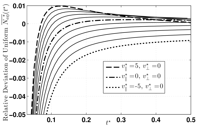
Figure 1: The relative deviation in $\overline{{N_{a}}_{0}^{\star}}\left(t^{\star}\right)$ from the true value (10) at the receiver when the uniform concentration assumption (18) is applied. The flow $v^{\star}_{\scriptscriptstyle\parallel}$ is varied from $-5$ to $5$ in increments of $1$.

In Fig. 2, we assess the uniform concentration assumption over time while varying $v^{\star}_{\perp}$ from $0$ to $5$ (by symmetry, $\overline{{N_{a}}_{0}^{\star}}\left(t^{\star}\right)$ due to $v^{\star}_{\perp}<0$ is equal to that due to $v^{\star}_{\perp}>0$). Similar to $v^{\star}_{\scriptscriptstyle\parallel}<0$, which is also a disruptive flow, a nonzero $v^{\star}_{\perp}$ increases the time that $\overline{{N_{a}}_{0}^{\star}}\left(t^{\star}\right)$ is underestimated. However, this does not significantly impact the general accuracy of the uniform concentration assumption, as the deviation for all flows shown is no more than $1.7\,\%$ for all $t^{\star}>0.1$.

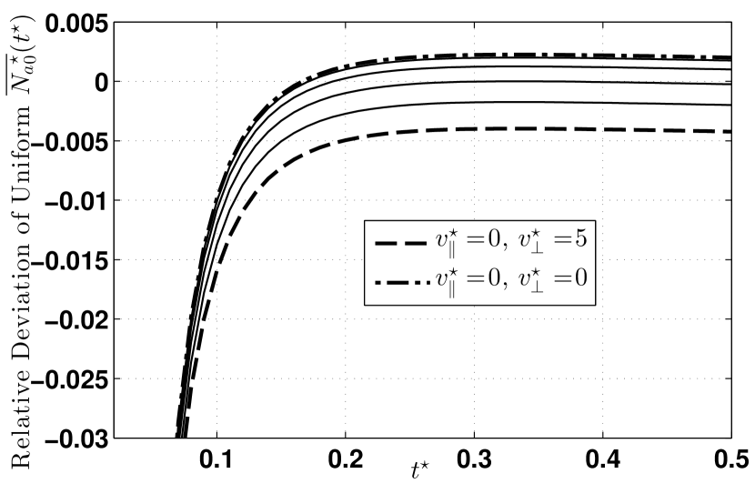
Figure 2: The relative deviation in $\overline{{N_{a}}_{0}^{\star}}\left(t^{\star}\right)$ from the true value (10) at the receiver when the uniform concentration assumption (18) is applied. The flow $v^{\star}_{\perp}$ is varied from $0$ to $5$ in increments of $1$.

In summary, we observe that the uniform concentration assumption cannot be universally applied to all degrees of flow at any time with a high degree of accuracy. The deviation of the assumption generally increases with the magnitude of the flow, and the assumption is least accurate immediately after the release of molecules by the transmitter. The benefit of the assumption is analytical tractability and simplicity in comparing the performance of detectors. To maximize accuracy, we do not apply the uniform concentration assumption in the evaluation of (10) in the remainder of this paper.

V-B Detector Performance

Our simulations to assess detector performance as a function of flow are executed in the particle-based stochastic framework that we described in [17, 18], and the environment parameters are listed in Table I. For simplicity, the $M$ observations are equally spaced within each bit interval. The chosen $D_{A}$ is similar to the diffusion coefficient of many small molecules in water at room temperature (see [19, Ch. 5]), and is also comparable to that of small biomolecules in blood plasma (see [20]). For reference, a maximum of $3.08$ molecules is expected from a single emission in the no-flow case $0.042\,\textnormal{m}\textnormal{s}$ after the molecules are released. If we set $L=x_{0}$, then $r_{obs}^{\star}=0.1$, the dimensionless bit interval is $0.8$, and advection $v^{\star}=1$ translates to a steady flow of $2\,\frac{\textnormal{m}\textnormal{m}}{\textnormal{s}}$ (on the order of average capillary blood speed, from $0.1$ to $10\,\frac{\textnormal{m}\textnormal{m}}{\textnormal{s}}$; see [20]). A bit interval that is (dimensionlessly) close to $1$ means that it is close to both the typical diffusion time and advection time when $v^{\star}=1$.

TABLE I: System parameters used for evaluating detector performance

Parameter	Symbol	Value
$\#$ of molecules per emission	$N_{EM}$	$10^{4}$
Probability of binary $1$	$P_{1}$	$0.5$
Length of transmitter sequence	$B$	$100$ bits
Bit interval time	$T_{int}$	$0.2\,$ms
Diffusion coefficient [19, 20]	$D_{A}$	$10^{-9}\frac{\textnormal{m}^{2}}{\textnormal{s}}$
Location of transmitter	$x_{0}$	$0.5\,\mu\textnormal{m}$
Radius of receiver	$r_{obs}$	$50\,$nm
Expected impact of noise source(s)	$\overline{{N_{A}}_{n}}\left(t\right)$	$1$ molecule
Simulation step size	$\Delta t$	$0.5\,\mu\textnormal{s}$

In the following figures, we consider the optimal sequence detector, the matched filter detector, and the equal weight detector. The expected error probabilities (evaluated using [8, Eq. 44]) and those found via simulation are averaged over all $100$ bits in the transmitter sequence and averaged over $1000$ bit sequences. The accuracy of the expected bit error probability decreases slightly as $M$ increases, because the assumption that the samples are independent becomes less valid.

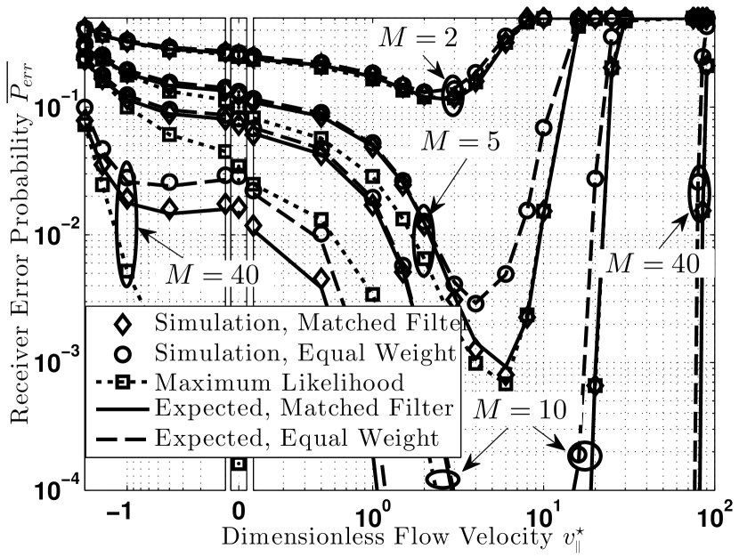
Figure 3: Receiver error probability as a function of $v^{\star}_{\scriptscriptstyle\parallel}$ for $M=\{2,5,10,40\}$ observations in each bit interval ($v^{\star}_{\perp}=0$). The horizontal axis is separated into 3 regions in order to show logarithmic scales: $-2\leq v^{\star}_{\scriptscriptstyle\parallel}\leq-0.2$ on a log scale, $v^{\star}_{\scriptscriptstyle\parallel}=0$, and $0.2\leq v^{\star}_{\scriptscriptstyle\parallel}\leq 100$ on a log scale.

In Fig. 3, we consider the impact of varying $v^{\star}_{\scriptscriptstyle\parallel}$, i.e., the flow is either in the direction of information transmission or directly opposite. The performance of all three detectors is quite similar for low $M$ and any value of $v^{\star}_{\scriptscriptstyle\parallel}$, but the optimal detector can become orders of magnitude better than the weighted sum detectors for large $M$, i.e., $M>10$. Generally, all detectors improve over the no-flow case when $v^{\star}_{\scriptscriptstyle\parallel}>0$. As $v^{\star}_{\scriptscriptstyle\parallel}$ increases, advection dominates diffusion and the impact of ISI is mitigated. However, with sufficiently high $v^{\star}_{\scriptscriptstyle\parallel}>0$, the molecules enter and leave the receiver between consecutive observations. As expected, communication degrades even though the flow is actually non-disruptive. We see this trend for $M=2$ when $v^{\star}_{\scriptscriptstyle\parallel}>2$, where the advection time ($L/v^{\star}_{\scriptscriptstyle\parallel}$, or $0.125$ ms for $v^{\star}_{\scriptscriptstyle\parallel}=2$) becomes on the order of the time between observations ($0.1$ ms). This trend continues for every value of $M$ as $v^{\star}_{\scriptscriptstyle\parallel}$ increases, but degradation would never occur as $v^{\star}_{\scriptscriptstyle\parallel}\to\infty$ if the receiver was perfectly synchronized to make an observation when the emitted molecules pass through. We also note that, in practice, a physical receiver would have receptors to which the emitted molecules could bind and then be observed. However, communication under a very strong flow could still degrade if the binding rate of the receptors was not sufficiently high.

All detectors fail when $v^{\star}_{\scriptscriptstyle\parallel}$ is negative and sufficiently large, since advection-dominant disruptive flow prevents all transmitted molecules from reaching the receiver. However, this degradation is less severe for small $v^{\star}_{\scriptscriptstyle\parallel}$ and, with sufficient sampling (i.e., $M=40$), Fig. 3 shows that both weighted sum detectors perform better (albeit slightly) than the no-flow case when $-1<v^{\star}_{\scriptscriptstyle\parallel}<-0.5$. Interestingly, the impact of this disruptive flow’s removal of $A$ molecules in their intended bit interval is mitigated by the removal of ISI molecules. Bi-directional transmission is thus possible in an environment with a steady flow moving in a direction parallel to the line between two transceivers, as long as advection does not dominate diffusion, and communication in each direction can be improved for some flows over the no-flow case if weighted sum detectors are used with a large number of samples.

In Fig. 4, we consider the impact of varying $v^{\star}_{\perp}$, i.e., the flow is perpendicular to the direction of information transmission. As might be expected, the impact of this disruptive flow is measurably different from $v^{\star}_{\scriptscriptstyle\parallel}<0$. For all $M>2$ shown, all detectors (including the maximum likelihood optimal sequence detector) have a range of $v^{\star}_{\perp}$ over which they perform better than in the no-flow case, and the potential for improvement increases with $M$. As with $v^{\star}_{\scriptscriptstyle\parallel}<0$, the impact of this disruptive flow’s removal of $A$ molecules in their intended bit interval is mitigated by the removal of ISI molecules, i.e., performance improves if the removal of ISI molecules is proportionately greater than the degradation of the useful signal. For example, the maximum improvement in the probability of error over the no-flow case is about $10\,\%$ at $v^{\star}_{\perp}=1$ when $M=5$, but the probability of error of the weighted sum detectors decreases by an order of magnitude when $M=40$ and $1.5\leq v^{\star}_{\perp}\leq 2$. The improvement in performance of the optimal sequence detector is small for all values of $M$ considered, although we expected no more than a small gain because this detector already accounts for ISI. As with negative $v^{\star}_{\scriptscriptstyle\parallel}$, all detectors eventually degrade as $v^{\star}_{\perp}$ increases and advection begins to dominate diffusion. However, the detectors do not appear to be as sensitive to $v^{\star}_{\perp}$ as they are to the corresponding negative values of $v^{\star}_{\scriptscriptstyle\parallel}$ in Fig. 3. As long as a flow moving in a direction perpendicular to the line between two transceivers does not dominate diffusion, bi-directional communication is not only possible, but can also be improved over the no-flow case if the detectors take enough samples.

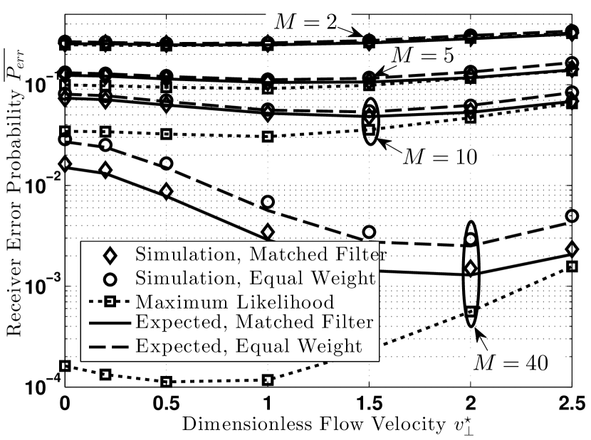
Figure 4: Receiver error probability as a function of $v^{\star}_{\perp}$ for $M=\{2,5,10,40\}$ observations in each bit interval ($v^{\star}_{\scriptscriptstyle\parallel}=0$).

Finally, in Fig. 5 we consider the impact of varying both $v^{\star}_{\scriptscriptstyle\parallel}$ and $v^{\star}_{\perp}$ simultaneously, such that $v^{\star}_{\scriptscriptstyle\parallel}=v^{\star}_{\perp}$. Detector performance is most similar to that shown in Fig. 3 because the detectors are more sensitive to $v^{\star}_{\scriptscriptstyle\parallel}$. However, there are two notable differences with Fig. 3. First, the improvement in the weighted sum detectors is slightly more pronounced in Fig. 5 when $M=40$ and both flows are small and negative; the expected bit error probability of the matched filter detector is a little more than $0.01$ when $v^{\star}_{\scriptscriptstyle\parallel}=v^{\star}_{\perp}=-0.5$ but almost $0.015$ when only $v^{\star}_{\scriptscriptstyle\parallel}=-0.5$. This is an example of disruptive flows in two dimensions contributing constructively. Second, the degradation of all detectors occurs sooner for positive $v^{\star}_{\scriptscriptstyle\parallel}$ and $v^{\star}_{\perp}$ than for positive $v^{\star}_{\scriptscriptstyle\parallel}$ alone; the probability of error for the equal weight detector and $M=5$ or $M=10$ begins increasing as a function of flow when $v^{\star}_{\scriptscriptstyle\parallel}=v^{\star}_{\perp}=2.5$, whereas it was still decreasing when only $v^{\star}_{\scriptscriptstyle\parallel}=2.5$. This is an example of the benefits of a non-disruptive flow component being mitigated by a disruptive flow component.

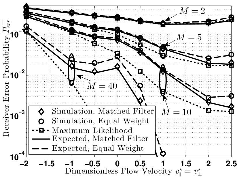
Figure 5: Receiver error probability as a function of $v^{\star}_{\scriptscriptstyle\parallel}=v^{\star}_{\perp}$ for the numbers of observations in each bit interval $M=\{2,5,10,40\}$.

VI Conclusions

In this paper, we studied the impact of steady uniform flow on a diffusive molecular communication system with a passive receiver. We derived the expected number of information molecules to be observed at the receiver when the transmitter is any distance away. A closed-form solution is available only when there is no flow component perpendicular to the direction of information transmission. We showed that there are conditions under which it is accurate to assume that the concentration of molecules expected at the receiver is uniform, thereby simplifying analysis. The simulation of detector performance showed that weighted sum detectors can perform better than in a no-flow environment when slow disruptive flows are present, and even optimal sequence detectors can perform slightly better than in a no-flow environment when there is a non-dominant disruptive flow perpendicular to the direction of information transmission. When flows become fast enough to dominate diffusion, disruptive flows prevent communication, whereas performance under a non-disruptive flow is only limited by the sampling times of the detector.

References

- [1] I. F. Akyildiz, F. Brunetti, and C. Blazquez, “Nanonetworks: A new communication paradigm,” Computer Networks, vol. 52, no. 12, pp. 2260–2279, May 2008.
- [2] T. Nakano, M. J. Moore, F. Wei, A. V. Vasilakos, and J. Shuai, “Molecular communication and networking: Opportunities and challenges,” IEEE Trans. Nanobiosci., vol. 11, no. 2, pp. 135–148, Jun. 2012.
- [3] G. A. Truskey, F. Yuan, and D. F. Katz, Transport Phenomena in Biological Systems, 2nd ed. Pearson Prentice Hall, 2009.
- [4] R. B. Bird, W. E. Stewart, and E. N. Lightfoot, Transport Phenomena, 2nd ed. John Wiley & Sons, 2002.
- [5] D. Miorandi, “A stochastic model for molecular communications,” Nano Commun. Net., vol. 2, no. 4, pp. 205–212, Dec. 2011.
- [6] S. Kadloor, R. R. Adve, and A. W. Eckford, “Molecular communication using Brownian motion with drift,” IEEE Trans. Nanobiosci., vol. 11, no. 2, pp. 89–99, Jun. 2012.
- [7] K. V. Srinivas, A. W. Eckford, and R. S. Adve, “Molecular communication in fluid media: The additive inverse Gaussian noise channel,” IEEE Trans. Inf. Theory, vol. 58, no. 7, pp. 4678–4692, Jul. 2012.
- [8] A. Noel, K. C. Cheung, and R. Schober, “Optimal receiver design for diffusive molecular communication with flow and additive noise,” Submitted to IEEE Trans. Nanobiosci., Jul. 2013. [Online]. Available: arXiv:1308.0109
- [9] H. ShahMohammadian, G. G. Messier, and S. Magierowski, “Nano-machine molecular communication over a moving propagation medium,” Nano Commun. Net., vol. 4, no. 3, pp. 142–153, Sep. 2013.
- [10] A. Noel, K. C. Cheung, and R. Schober, “Using dimensional analysis to assess scalability and accuracy in molecular communication,” in Proc. 2013 IEEE ICC MONACOM, Jun. 2013, pp. 818–823.
- [11] J. Crank, The Mathematics of Diffusion, 2nd ed. Oxford University Press, 1980.
- [12] H. C. Berg, Random Walks in Biology. Princeton University Press, 1993.
- [13] T. Szirtes, Applied Dimensional Analysis and Modeling, 2nd ed. Butterworth-Heinemann, 2007.
- [14] E. W. Ng and M. Geller, “A table of integrals of the error functions,” J. Res. Bur. Stand., vol. 73B, no. 1, pp. 1–20, Jan.-Mar. 1969.
- [15] M. J. Moore and T. Nakano, “Oscillation and synchronization of molecular machines by the diffusion of inhibitory molecules,” IEEE Trans. Nanotechnol., vol. 12, no. 4, pp. 601–608, Jul. 2013.
- [16] P. Nelson, Biological Physics: Energy, Information, Life, updated 1st ed. W. H. Freeman and Company, 2008.
- [17] A. Noel, K. C. Cheung, and R. Schober, “Improving diffusion-based molecular communication with unanchored enzymes,” in Proc. 2012 ICST BIONETICS, Dec. 2012. [Online]. Available: arXiv:1305.1783
- [18] ——, “Improving receiver performance of diffusive molecular communication with enzymes,” to appear in IEEE Trans. Nanobiosci., 2014. [Online]. Available: dx.doi.org/10.1109/TNB.2013.2295546
- [19] E. L. Cussler, Diffusion: Mass transfer in fluid systems. Cambridge University Press, 1984.
- [20] A. A. Merrikh and J. L. Lage, “Effect of blood flow on gas transport in a pulmonary capillary,” Journal of Biomech. Eng., vol. 127, no. 3, pp. 432–439, Jun. 2005.