A skew Gaussian decomposable
graphical model

Abstract

This paper propose a novel decomposable graphical model to accommodate skew Gaussian graphical models. We encode conditional independence structure among the components of the multivariate closed skew normal random vector by means of a decomposable graph and so that the pattern of zero off-diagonal elements in the precision matrix corresponds to the missing edges of the given graph. We present conditions that guarantee the propriety of the posterior distributions under the standard noninformative priors for mean vector and precision matrix, and a proper prior for skewness parameter. The identifiability of the parameters is investigated by a simulation study. Finally, we apply our methodology to two data sets.

Keywords: Decomposable graphical models; multivariate closed skew normal distribution; Conditional independence; Noninformative prior.

1 Introduction

In recent years, there have been many developments in multivariate statistical models. Making sense of all the many complex relationships and multivariate dependencies present in the data, formulating correct models and developing inferential procedures is an important challenge in modern statistics. In this context, graphical models currently represent an active area of statistical research which have served as tools to discover structure in data. More specifically, graphical models are multivariate statistical models in which the corresponding joint distribution of a family of random variables is restricted by a set of conditional independence assumptions, and the conditional relationships between random variables are encoded by means of a graph. In the Gaussian case, these models induce the conditional independence assumptions by zeros in the precision matrix. An important reason for working with this class of distributions is important properties like closure under marginalization, conditioning and linear combinations which is seldom preserved outside the class of multivariate normal distributions. However, in spite of substantial advances, the Gaussian distributional assumption might be overly restrictive to represent the data. The real data could be highly non-Gaussian and may show features like skewness.

In this article, we study skew distributions in graphical models with the aim of mimicking the success of Gaussian graphical models as much as possible. The last decade has witnessed major developments in models whose finite dimensional marginal distributions are multivariate skew-normal. Azzalini and Capitanio (1999) introduced multivariate skew-normal (SN) distribution which enjoys some of the useful properties of normal distribution, such as property of closure under marginalization and conditioning. Accordingly, an $n$-dimensional random vector ${\bf{Y}}$ is said to have a SN distribution if its density is

$$\phi_{n}({\bf{y}};{\boldsymbol{\mu}},\Omega)\Phi(\alpha_{0}+{\bf\alpha}^{\prime}D_{\Omega}^{-1}({\bf{y}}-{\boldsymbol{\mu}}))/\Phi(\tau),$$

where $\phi_{n}(\cdot;{\boldsymbol{\mu}},\Omega)$ is the probability density function of the $n$-dimensional $N_{n}({\boldsymbol{\mu}},\Omega)$ variable, $\Phi(\cdot)$ is cumulative distribution function of $N(0,1)$, ${\boldsymbol{\mu}}\in\Re^{n}$, $\tau\in\Re$, $\Omega\in\Re^{n\times n}$ is a full rank covariance matrix, $D_{\Omega}=diag(\Omega_{11},\cdots,\Omega_{nn})^{1/2}$, ${\boldsymbol{\alpha}}\in\Re^{n}$ is shape parameter and $\alpha_{0}=\tau(1+{\boldsymbol{\alpha}}^{\prime}D_{\Omega}^{-1}\Omega D_{\Omega}^{-1}{\boldsymbol{\alpha}})^{1/2}$. When ${\boldsymbol{\alpha}}={\bf 0}$ we are back to the multivariate normal distribution. Capitanio et al. (2003) used the SN family in graphical models examining in particular the construction of conditional independence graphs. Their results show that if ${\bf Y}$ be an n-variate SN distribution with covariance matrix $\Omega$ and skewness vector ${\boldsymbol{\alpha}}$, then

$$Y_{i}\perp Y_{j}|{\bf Y}_{-ij}\ \ \Leftrightarrow\ \ \Omega^{ij}=0\ \ and\ \ \alpha_{i}\alpha_{j}=0$$

where ${\bf Y}_{-ij}$ is ${\bf Y}$ with the $i$th and $j$th elements deleted and $\Omega^{ij}$ denotes the $(i,j)$th entry of $\Omega^{-1}$. Comparing with the Gaussian graphical model, an extra constraint $\alpha_{i}\alpha_{j}=0$ is necessary to capture conditional independence property. It means if we believe $Y_{i}$ and $Y_{j}$ are conditionally independent then at least one of $\alpha_{i}$ and $\alpha_{j}$ must be zero. Hence, applying this constraint in practical issues is challenging. Alternatively, Dominguez-Molina et al. (2003) and Gonzalez-Farias et al. (2004) proposed the multivariate closed skew normal (CSN) distribution which includes the property of SN family. Also unlike the SN family, the CSN family enjoys this property that the joint distribution of i.i.d. CSN random variables is the multivariate CSN distribution.

Although much progress has been made in the context of skew normal distributions, the achieved successes in graphical models are limited. The preservation of conditional independence property for skew normal variables has shown that the extending the class of skew-normal distributions to graphical models is challenging. The aim of this paper is to develop a multivariate closed skew normal graphical model. We encode conditional independence structure among the components of the multivariate closed skew normal random vector with respect to a decomposable graph $G$. The main motivation to use the decomposable graphs for encoding the conditional independence is that for this type of graph there exists an ordering of the vertices such that the zero elements in precision matrix are reflected in its Cholesky decomposition (Paulsen et al., 1989). Under decomposable graphs, the conditional independence property is maintained for our skewed graphical model, and simplification occurs in both the interpretation of data and the estimation procedure. Models can be specified in terms of conditional and marginal probability distributions, leading to a simplified analysis based on lower dimensional components (Giudici and Green, 1999; Letac and Massam, 2007; Khare and Rajaratnam, 2011).

The precision matrix is the fundamental object that evaluates conditional dependence between random variables. Estimating a sparse precision matrix is crucial specially in high-dimensional problems. In this context, a family of conjugate prior distributions for the precision matrix is developed. Conditions for propriety of the posterior are given under the standard noninformative priors on mean vector and precision matrix as well as a proper prior for the skewness parameter. We also develop and implement a Markov chain Monte Carlo (MCMC) sampling approach for inference.

The organization of the paper is as follows. Section 2 introduces the required preliminaries and notation. In Section 3, a novel skew Gaussian decomposable graphical model is constructed using a multivariate closed skew normal distribution and its properties are established. Section 4 discusses Bayesian analysis using Gibbs sampling to sample from the posterior distribution. A simulation study is reported in Section 5. Section 6 illustrates the use of proposed methodology in two real data sets: an analysis of student marks from Mardia et al. (1979) and an analysis of the carcass data from gRbase package of R. Finally, conclusions and discussion are given in Section 7. The Appendix contains proofs of some of the results in the main text.

2 Preliminaries

2.1 Multivariate closed skew-normal distribution

An $n$-dimensional random vector ${\bf{Y}}$ is said to have a multivariate closed skew-normal distribution, denoted by $CSN_{n,m}({\boldsymbol{\mu}},\Sigma,\Gamma,{\boldsymbol{\nu}},\Delta)$, if its density function is of the form

$$f({\bf y})=\phi_{n}({\bf{y}};{\boldsymbol{\mu}},\Sigma)\Phi_{m}(\Gamma({\bf{y}}-{\boldsymbol{\mu}});{\boldsymbol{\nu}},\Delta)/\Phi_{m}(0;{\boldsymbol{\nu}},\Delta+\Gamma\Sigma\Gamma^{\prime}),$$ (1)

where ${\boldsymbol{\mu}}\in\Re^{n}$, ${\boldsymbol{\nu}}\in\Re^{m}$, and $\Sigma\in\Re^{n\times n}$ and $\Delta\in\Re^{m\times m}$ are both covariance matrices, $\Gamma\in\Re^{m\times n}$, and $\Phi_{n}(\cdot;{\boldsymbol{\mu}},\Sigma)$ is the cumulative distribution function of the $n$-dimensional normal distribution with mean vector ${\boldsymbol{\mu}}$ and covariance matrix $\Sigma$. To derive this distribution, Gonzalez-Farias et al. (2004) consider a $(n+m)$-dimensional normal random vector

$$(W_{0_{1}},\cdots,W_{0_{m}},W_{1},\cdots,W_{n})^{\prime}=\left(\begin{array}[]{c}{\bf W_{0}}\\ {\bf W}\\ \end{array}\right)\sim N_{n+m}\left(\begin{array}[]{cc}{\bf 0},&\left(\begin{array}[]{cc}\Delta+\Gamma\Sigma\Gamma^{\prime}&\Gamma\Sigma\\ \Sigma\Gamma^{\prime}&\Sigma\\ \end{array}\right)\\ \end{array}\right).$$

Then, the probability density function of ${\bf Y}=({\bf W}|{\bf W}_{0}>{\boldsymbol{\nu}})$ is the multivariate closed skew-normal (1). If $\Gamma=0$ and $m=1$, this density reduces to the multivariate normal one and the skew-normal distribution (Azzalini, 2005), respectively. Allard and Naveau (2007) used the multivariate closed skew normal and introduced a spatial skewed Gaussian process as a novel way of modeling skewness for spatial data. To increase the amount of skewness in the vector ${\bf{Y}}$ as well as to simplify the interpretation of this density, they assumed that $m=n$, ${\boldsymbol{\nu}=0}$, $\Delta=\Sigma$ and $\Gamma=\alpha I_{n}$ in which $\alpha\in\Re$ is a single parameter controlling skewness and $I_{n}$ is the identity matrix of order $n$. This model is also referred to as the homotopic model.

We will make use of the alternative representation of Dominguez-Molina et al. (2003) for CSN families,

$${\bf{Y}}\stackrel{{\scriptstyle d}}{{=}}{\boldsymbol{\mu}}+(\Sigma^{-1}+\Gamma^{\prime}\Delta^{-1}\Gamma)^{-\frac{1}{2}}{\bf V}+\Sigma\Gamma^{\prime}(\Delta+\Gamma\Sigma\Gamma^{\prime})^{-1}{\bf U},$$ (4)

where ${\bf V}$ and $\bf{U}$ are independent multivariate normal distribution $N_{n}(0,I_{n})$ and a multivariate truncated normal distribution $TN_{n}(0;0,\Delta+\Gamma\Sigma\Gamma^{\prime})$, respectively, where $TN_{n}({\bf{c}};{\boldsymbol{\mu}},\Sigma)$ denotes the $N_{n}({\boldsymbol{\mu}},\Sigma)$ distribution truncated below at the vector ${\bf{c}}$. Also, if ${\bf Y}$ is partitioned as ${\bf Y}=({\bf Y}^{\prime}_{1},{\bf Y}_{2}^{\prime})^{\prime}$, then the conditional distribution of $(n-k)$-dimensional vector ${\bf Y}_{2}$ given ${\bf Y}_{1}={\bf y}_{1_{0}}$ is

$$CSN_{n-k,m}({\boldsymbol{\mu}}_{2}+\Sigma_{21}\Sigma_{11}^{-1}({\bf y}_{1_{0}}-{\boldsymbol{\mu}}_{1}),\Sigma_{22.1},\Gamma_{2},{\boldsymbol{\nu}}-\Gamma^{*}({\bf y}_{1_{0}}-{\boldsymbol{\mu}}_{1}),\Delta),$$

where $\Sigma_{22.1}=\Sigma_{22}-\Sigma_{21}\Sigma_{11}^{-1}\Sigma_{12}$, $\Gamma^{*}=\Gamma_{1}+\Gamma_{2}\Sigma_{21}\Sigma_{11}^{-1}$ and the parameters are induced corresponding to the partition of ${\bf Y}$ as

$${\boldsymbol{\mu}}=\left(\begin{array}[]{c}{\boldsymbol{\mu}}_{1}\\ {\boldsymbol{\mu}}_{2}\\ \end{array}\right),\ \ \ \ \ \ \Sigma=\left(\begin{array}[]{cc}\Sigma_{11}&\Sigma_{12}\\ \Sigma_{21}&\Sigma_{22}\\ \end{array}\right),\ \ \ \ \ \ \Gamma=\left(\begin{array}[]{cc}\Gamma_{1}&\Gamma_{2}\\ \end{array}\right).$$

2.2 Graph theory

Let $V$ be a finite set of vertices and $E=\{(u,v):u,v\in V,u\neq v\}$ be a set of edges so that $E\subseteq V\times V$. Define a graph $G$ as an ordered pair $G=(V,E)$ of vertices and edges, where $V$ is assumed to be finite. When $(u,v)\in E$, we say that $u$ and $v$ are adjacent in $G$. A graph is said to be complete if all the vertices are adjacent to each other. It is understood that $(u,v)\in E$ implies $(v,u)\in E$, i.e., the edges are undirected. For an undirected graph $G=(V,E)$, we say that $u$ and $v$ are neighbors when $(u,v)\in E$. For any $A\subset V$, a subgraph of $V$ is defined as the graph $G_{A}=(A,E\cap(A\times A))$. A path from $v_{1}$ to $v_{m}$ is a sequence of distinct vertices in $V$, $v_{1},v_{2},\cdots,v_{m}$, for which $(v_{j},v_{j+1})\in E$ for $j=1,\cdots,m-1$. A subset $C\subset V$ separates two vertices $i\notin C$ and $j\notin C$, if every path from $i$ to $j$ contains at least one vertex from $C$. A clique of $G$ is a complete subgraph of $G$. A subgraph is a maximal clique if it is not contained in a larger complete subgraph. Any path that begins and ends at the same vertex is called a cycle. A tree is a connected graph with no cycles.

Definition 1: (Decomposable graph (Lauritzen, 1996)) An undirected graph is said to be decomposable if any induced subgraph does not contain a cycle of length greater than or equal to four.

Figure 1 shows examples of non-decomposable and decomposable graphs. Decomposable graphs have several characterizations in terms of vertex orderings.

Definition 2: For an undirected graph $G=(V,E)$, an ordering $\gamma:V\mapsto\{v_{1},\cdots,v_{m}\}$ of $m$ vertices $(1,\cdots,m)$ is known as a perfect vertex elimination scheme for G if for every triplet $v_{i},v_{j},v_{k}$ with $1\leq i<j<k\leq m$ the following condition holds:

$$(\gamma^{-1}(v_{j}),\gamma^{-1}(v_{i}))\in E,\ \ (\gamma^{-1}(v_{k}),\gamma^{-1}(v_{i}))\in E\ \ \Rightarrow\ \ (\gamma^{-1}(v_{k}),\gamma^{-1}(v_{j}))\in E.$$

In Figure 1(b), we show examples of perfect vertex elimination schemes for some decomposable graphs. The existence of such an ordering is an important advantage of decomposable over nondecomposable graphs, and the existence of this ordering characterize decomposable graphs. More formally, every decomposable graph admits an ordering of vertexes in terms of its cliques which is a perfect vertex elimination scheme. If for an undirected graph $G$, there exists an ordering of its vertices corresponding to a perfect vertex elimination scheme, then $G$ is a decomposable graph (Lauritzen, 1996, page 18). However, this ordering need not be unique. A constructive way to obtain such an ordering is given in Lauritzen (1996).

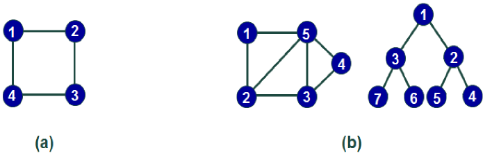
Figure 1: (a) A non-decomposable graph, and (b) two decomposable graphs.

Definition 3: (Modified Cholesky decomposition) If $Q$ is a positive definite matrix, then there exists a unique decomposition

$$Q=L^{\prime}DL$$

where $L$ is a upper triangular matrix with unit diagonal entries and $D$ a diagonal matrix with positive diagonal entries. The Cholesky decomposition of $Q$ is $\Gamma^{\prime}\Gamma$ where $\Gamma=D^{\frac{1}{2}}L$ is called the Cholesky triangle.

The following lemma will play a central role in our work.

Lemma 1: (Paulsen et al. 1989) Let $\Omega$ be an arbitrary positive definite matrix with zero restrictions according to decomposable graph $G=(V,E)$, i.e., $\Omega_{ij}=0$ whenever $(i,j)\notin E$. Then there exists an ordering of the vertices such that if $\Omega=L^{\prime}DL$ is the modified Cholesky decomposition corresponding to this ordering, then for $i<j$,

$$L_{ij}=0\Leftrightarrow(i,j)\notin E.$$

Hence, the zeros in $\Omega$ are preserved in the lower triangle of the corresponding matrix $L$ obtained from the modified Cholesky decomposition. We assume from now on that graph $G$ is decomposable.

An $m$-dimensional Gaussian graphical model can be represented by the class of multivariate normal distributions with fixed zeros in the precision matrix (i.e., conditional independencies) described by a given graph $G=(V,E)$ where the number of vertices is $m$. That is, if $(i,j)\notin E$, the $i$th and $j$th components of the multivariate random vector are conditionally independent.

We now introduce some notations and spaces from Khare and Rajaratnam (2011). Let $M_{m}^{+}$ and $M_{m}$ denote the cone of symmetric positive definite matrices of order $m$ and symmetric positive semidefinite matrices of order $m$, respectively, then the two parameter sets $P_{G}^{m}$ and $SP_{G}^{m}$ according to decomposable graph $G=(V,E)$ are defined as

$$P_{G}^{m} = \{\Omega\in M_{m}^{+}\ |\ \Omega_{ij}=0,\ \ (i,j)\notin E\},$$

$$SP_{G}^{m} = \{\Omega\in M_{m}\ |\ \Omega_{ij}=0,\ \ (i,j)\notin E\},$$

and also define

$$\ell_{G}^{m} = \{L:\ \ L_{ij}=0\ \ whenever\ i>j,\ or\ (i,j)\notin E\ and\ L_{ii}=1\ \forall\ 1\leq i,j\leq m\},$$

$$\Theta_{G}^{m} = \{\theta=(L,D):\ \ L\in\ell_{G}^{m}\ \ and\ D\ diagonal\ with\ D_{ii}>0\ \forall\ 1\leq i\leq m\}.$$

3 Skew Gaussian decomposable graphical models

To introduce a skew version of $k$-dimensional Gaussian graphical (GG) model, we first consider the following tree graphical model in a loose and imprecise form

$${\stackrel{{\scriptstyle 1}}{{\bigcirc}}}\line(1,0){30.0}\stackrel{{\scriptstyle 2}}{{\bigcirc}}\line(1,0){30.0}\stackrel{{\scriptstyle 3}}{{\bigcirc}}.$$ (6)

Based on this graph, let ${\bf X}=(X_{1},X_{2},X_{3})$ be a random vector whose elements are indexed by graph (6). We introduce three independent increments

$$\epsilon_{1}=\kappa_{1}X_{1},\ \ \ \ \epsilon_{2}=\kappa_{2}(X_{2}-b_{12}X_{1}),\ \ \ \ \epsilon_{3}=\kappa_{3}(X_{3}-b_{23}X_{2}).$$

where $\kappa_{1},\kappa_{2},\kappa_{3}\in\Re^{+}$ and $b_{12},b_{23}\in\Re$. Now, we can relate ${\boldsymbol{\epsilon}}=(\epsilon_{1},\epsilon_{2},\epsilon_{3})$ to ${\bf X}=(X_{1},X_{2},X_{3})$ by ${\boldsymbol{\epsilon}}=D_{\kappa}^{\frac{1}{2}}B{\bf X}$ where

$$B=\left(\begin{array}[]{ccc}1&0&0\\ -b_{12}&1&0\\ 0&-b_{23}&1\\ \end{array}\right),\ \ \ \ \ and\ \ \ \ D_{\kappa}=diag(\kappa_{1}^{2},\kappa_{2}^{2},\kappa_{3}^{2}).$$

If we suppose $\epsilon_{1},\epsilon_{2},\epsilon_{3}\stackrel{{\scriptstyle iid}}{{\sim}}N(0,1)$, then the joint density of ${\bf X}=(X_{1},X_{2},X_{3})$ becomes trivariate normal distribution with fixed zeros in the precision matrix described by given graph. Our aim is to assess the suitability and wider applicability of asymmetric distributions in graphical models with the hope of mimicking the success of Gaussian graphical models as much as possible. To do this, we need to study the following two questions

• How can we choose a skewed distribution for $\boldsymbol{\epsilon}$ such that the distribution of ${\bf X}$ belong to the same class as that of the $\boldsymbol{\epsilon}$?

• What conditions are necessary to achieve the Markov property for the skewed graphical model?

To address these questions, we will use the CSN model that is more general than SN, and is closed under marginalization, conditioning and linear combination. Also unlike the SN family the joint distribution of i.i.d. CSN random variables is a multivariate CSN distribution. We now assume

$$\epsilon_{i}\sim CSN_{1,1}(0,1,\alpha_{i},0,1),\ \ \ \ i=1,2,3\ \ \Leftrightarrow\ \ {\boldsymbol{\epsilon}}\sim CSN_{3,3}({\bf 0},I_{3},D_{\alpha},{\bf 0},I_{3})$$

where $D_{\alpha}=diag(\alpha_{1},\alpha_{2},\alpha_{3})$. Note that $\alpha_{i}$ is interpreted as skewness parameters of the $i$th increment. Using the closure property of the CSN distribution under linear transformations, the joint density for ${\bf X}$ becomes

$$p({\bf x})=2^{3}\phi_{3}({\bf{x}};0,(B^{\prime}D_{\kappa}B)^{-1})\Phi_{3}(D_{\alpha}B{\bf{x}};{\bf 0},D_{\kappa}^{-1}).$$

In this example, we can easily show that $X_{1}\perp X_{3}|X_{2}$, so we have the Markov property. The question is then: how can we extend this easy example to a more general graphical model? This we will study next.

Definition 4: Consider an undirected decomposable graph $G=(V,E)$ where the number of vertices is $k$ and ordering of the vertices corresponds to a perfect vertex elimination scheme. A random vector ${\bf X}=(X_{1},\cdots,X_{k})^{\prime}$ is called a skew Gaussian decomposable graphical (SGDG) model with respect to graph $G$ with mean ${\boldsymbol{\mu}}\in\Re^{k}$, the precision matrix $Q\in P_{G}^{k}$ and the skewness parameters $\boldsymbol{\alpha}\in\Re^{k}$, if its density is $CSN_{k,k}({\boldsymbol{\mu}},Q^{-1},D_{\alpha}L,{\bf 0},D_{\kappa}^{-1})$ or equivalently

$$p({\bf x}) = 2^{k}\phi_{k}({\bf{x}};{\boldsymbol{\mu}},Q^{-1})\Phi_{k}(D_{\alpha}L({\bf{x}}-{\boldsymbol{\mu}});{\bf 0},D_{\kappa}^{-1})$$ (8)

$$= (\frac{2}{\pi})^{k/2}|D_{\kappa}|^{1/2}\exp({-\frac{1}{2}({\bf x}-{\boldsymbol{\mu}})^{\prime}Q({\bf x}-{\boldsymbol{\mu}})})\Phi_{k}(D_{\alpha}L({\bf x}-{\boldsymbol{\mu}});{\bf 0},D_{\kappa}^{-1}),$$

where $D_{\kappa}=diag(\kappa_{1}^{2},\cdots,\kappa_{k}^{2})$, $D_{\alpha}=diag(\alpha_{1},\cdots,\alpha_{k})$ and $(L,D_{\kappa})\in\Theta_{G}^{k}$ and correspond to modified Cholesky decomposition of $Q$.

Figure 2: Left: contour plot of the SGDG model with parameters ${\boldsymbol{\mu}=(0,0)^{\prime}}$, $D_{\kappa}=diag(1,1)$, $L_{12}=-0.5$ and $\alpha_{1}=\alpha_{2}=2$. Right: contour plot of the SGDG model with parameters ${\boldsymbol{\mu}=(0,0)^{\prime}}$, $D_{\kappa}=diag(1,1)$, $L_{12}=-0.5$ and $\alpha_{1}=\alpha_{2}=4$.

When skewness parameters are all zero, the density (8) reduces to the multivariate normal. Figure 2 shows contour plots of the SGDG model ($k=2$) for different skewness parameters. Although Definition 4 depends on the ordering of the vertices, this is not as restrictive as it first appears. The ordering is essentially another parameter to be specified and can be viewed as imposing extra information. In sequel, we show that the SGDG model is supported by the property of conditional independence.

Theorem 1: Let ${\bf X}$ be closed skew-normal distributed corresponding to Definition 4. Then for $i<j$, we have

$$X_{i}\perp X_{j}|{\bf x}_{-ij}\ \ \Leftrightarrow\ \ Q_{ij}=0\ \ \Leftrightarrow\ \ L_{ij}=0\ \ \Leftrightarrow\ \ (i,j)\notin E.$$

This is one of the main results. It simply says that similar to the Gaussian graphical models the nonzero pattern of $Q$ determines $G$, so we can read off from $Q$ whether $X_{i}$ and $X_{j}$ are conditionally independent, so the natural way to parametrize the SGDG model is by its precision matrix $Q$. Although, the results in this article are based on decomposable graphical models, in sequel we have a theorem based on an arbitrary undirected graph.

Lemma 2: Consider an arbitrary undirected graph $G=(V,E)$ where $V=\{1,2,\cdots,k\}$. Let $L$ be the modified cholesky decomposition of the precision matrix corresponding to graph $G$. Define the set $F(i,j)=\{i+1,\cdots,j-1,j+1,\cdots,k\}$. Now, if $F(i,j)$ separates $i<j$ in $G$, then $L_{ij}=0$ (see Rue and Held, 2005).

Theorem 2: Consider an arbitrary undirected graph $G=(V,E)$. Let $L$ be the modified Cholesky triangle of precision matrix $Q\in P_{G}^{k}$. Suppose ${\bf X}$ is closed skew-normal distributed (8), then for $i<j$, we have

$$if\ F(i,j)\ separates\ two\ vertices\ i\ and\ j\ \ \Rightarrow\ \ X_{i}\perp X_{j}|{\bf x}_{-ij}.$$

Alternatively, using the representation of Dominguez-Molina et al. (2003) for CSN families, a stochastic representation of the SGDG model is

$${\bf X}\stackrel{{\scriptstyle d}}{{=}}{\boldsymbol{\mu}}+L^{-1}D_{\kappa}^{-\frac{1}{2}}D_{\alpha}(I+D^{2}_{\alpha})^{-\frac{1}{2}}{\bf U}+L^{-1}D_{\kappa}^{-\frac{1}{2}}(I+D^{2}_{\alpha})^{-\frac{1}{2}}{\bf V},$$ (9)

where ${\bf V}$ and ${\bf U}$ are independent multivariate normal distribution $N_{k}({\bf 0},I_{k})$ and a multivariate half-normal distribution $HN_{k}({\bf 0},I_{k})$, respectively. From a computational point of view, this representation is useful because it implies that an random vector distributed according to (8) can be generated using two independent normal random vectors. The mean vector and covariance matrix of ${\bf X}$ is

$$E({\bf X}) = {\boldsymbol{\mu}}+L^{-1}D_{\kappa}^{-\frac{1}{2}}D,$$

$$Cov({\bf X}) = (L^{\prime}D_{\kappa}^{\frac{1}{2}}(I_{k}-D^{2})D_{\kappa}^{\frac{1}{2}}L)^{-1}$$

where diagonal matrix $D$ is $D=\sqrt{\frac{2}{\pi}}D_{\alpha}(I_{k}+D^{2}_{\alpha})^{-\frac{1}{2}}$. Hence, the zero elements of inverse of covariance matrix ${\bf X}$ are the same of those of the precision matrix $Q$.

4 Bayesian analysis

In this section, we will discuss Bayesian inference of the SGDG model (8). Assume $n$ independent observations ${\bf x}=({\bf x}_{1},\cdots,{\bf x}_{n})$ from this model. We use the representation (9) and the following hierarchical representation

$${\bf X}_{j}|{\bf U}_{j} \sim N_{k}({\boldsymbol{\mu}}+L^{-1}D_{\delta}{\bf U}_{j},(L^{\prime}D_{\omega}L)^{-1}),\ \ \ \ {\boldsymbol{\delta}},\ {\boldsymbol{\mu}}\in\Re^{k},\ \ (L,D_{\omega})\in\Theta_{G}$$

$${\bf U}_{j} \sim HN_{k}({\bf 0},I_{k}),\ \ \ \ \ \ j=1,\cdots,n,$$ (10)

where $D_{\omega}=diag(\omega_{1}^{2},\cdots,\omega_{k}^{2})$ and $D_{\delta}=diag(\delta_{1},\cdots,\delta_{k})$ with $\delta_{i}=\frac{\alpha_{i}}{\kappa_{i}\sqrt{1+\alpha_{i}^{2}}}$ and $\omega_{i}={\kappa_{i}\sqrt{1+\alpha_{i}^{2}}}$. The later reparametrization has been imposed to ease the computations. We will now discuss the prior distribution for the unknown parameters ${\boldsymbol{\eta}}=({\boldsymbol{\mu}},{\boldsymbol{\delta}},L,D_{\omega})$. With regard to relation between $\delta_{i}$ and $\omega_{i}$ in the mentioned reparametrization (i.e. $\delta_{i}=\frac{\alpha_{i}}{\omega_{i}}$), we will use a correlated prior for ${\boldsymbol{\delta}}=(\delta_{1},\cdots,\delta_{k})$ and ${\boldsymbol{\omega}}=(\omega_{1},\cdots,\omega_{k})$;

$$\pi({\boldsymbol{\delta}}|{\boldsymbol{\omega}})=N_{k}({\bf 0},b_{1}D_{\omega}^{-1}),$$

where $b_{1}\in\Re_{+}$ is fixed. For the priors on ${\boldsymbol{\mu}}\in\Re^{k}$ and $(L,D_{\omega})\in\Theta_{G}$. We will discuss two separate prior structures corresponding to independent proper and noninformative priors for these parameters.

Independent proper priors on ${\boldsymbol{\mu}}$, ${\boldsymbol{\omega}}^{2}$ and $L$: We take normal priors for mean vector and lower triangular matrix and gamma prior for precision parameters as follows

$$\pi({\boldsymbol{\mu}}) = N_{k}({\boldsymbol{\mu}}_{0},b_{2}I_{k}),$$

$$\pi({\boldsymbol{\omega}}^{2}) = \prod_{i=1}^{k}G(b_{3},b_{4}),$$

$$\pi(L_{1.}^{\neq 0},\cdots,L_{k-1.}^{\neq 0}) = \prod_{i=1}^{k-1}N_{||N^{\prec}(i)||}({\boldsymbol{0}},b_{5}I_{||N^{\prec}(i)||}),$$ (11)

where $G(a,b)$ denotes the gamma distribution, $L_{i.}^{\neq 0}=(L_{ij})_{\{i<j,\ (i,j)\in E\}}$ denotes the nonzero off-diagonal elements of $i$’th row of $L$ and $N^{\prec}(i):=\{j:\ (i,j)\in E,i<j\}$. Also, ${\boldsymbol{\mu}}_{0}\in\Re^{k}$ and $b_{i}\in\Re_{+},i=2,3,4,5,$ are known hyperparameters.

Non-informative priors on ${\boldsymbol{\mu}}$, ${\boldsymbol{\omega}}^{2}$ and $L$: Assign a common noninformative prior distributions for the mean vector of the form $\pi({\boldsymbol{\mu}})\propto{1}$. Khare and Rajaratnam (2011) formed a rich and flexible class of Wishart priors for decomposable covariance graphs in Gaussian covariance graph models in which marginal independence among the components of a multivariate random vector is encoded by means of a graph $G$. They also considered the case where G is decomposable. Although covariance graph models are distinctly different from the traditional concentration graph models, after some modifications, their prior is extendable in our problem case. In this context, the class of measures on $(L,D_{\omega})\in\Theta_{G}$ is provided with density

$$\pi(L\in dL,D_{\omega}\in dD_{\omega})\propto\prod_{i=1}^{k}(\omega^{2}_{i})^{\psi_{i}/2-1}e^{-\frac{1}{2}tr((L^{\prime}D_{\omega}L)\Psi)}\prod_{i<j,(i,j)\in E}dL_{ij}\prod_{i=1}^{k}d\omega^{2}_{i},$$ (12)

where positive definite matrix $\Psi$ and $\psi_{i}\in\Re_{+},\ i=1,\cdots,k$ are known hyperparameters. Theorem 3 provides a sufficient condition for the existence of a normalizing constant for $\pi(L,D_{\omega})$.

Theorem 3: Let $dL:=\prod_{i<j,(i,j)\in E}dL_{ij}$ and $dD_{\omega}:=\prod_{i=1}^{k}d\omega^{2}_{i}$. if $\psi_{i}>||N^{\prec}(i)||$, then

$$\int_{\Theta_{G}}\prod_{i=1}^{k}(\omega^{2}_{i})^{\psi_{i}/2-1}\exp\{-\frac{1}{2}tr((L^{\prime}D_{\omega}L)\Psi)\}dD_{\omega}dL<\infty.$$ (13)

A standard noninformative prior for lower triangular matrix $L$ and precision parameters ${\boldsymbol{\omega}}^{2}$ can be chosen by respecting the zeros for $\Psi$ and $\psi_{i},\ i=1,\cdots,k$. Hence, the resulting non-informative prior on ${\boldsymbol{\mu}}$, $L$ and ${\boldsymbol{\omega}}^{2}$ is of the form

$$\pi({\boldsymbol{\mu}},L,{\boldsymbol{\omega}}^{2})\propto\prod_{i=1}^{k}\frac{1}{\omega^{2}_{i}}.$$ (14)

Theorem 4 shows that the posterior distribution is proper under prior distribution (14). To show this, we use a result by Mouchart (1976) and Florens et al. (1990) which implies that the posterior distribution exists as a proper only when

$$p({\bf x})=\int p({\bf x}|{\boldsymbol{\mu}},{\boldsymbol{\omega}}^{2},{\boldsymbol{\delta}},L)\pi({\boldsymbol{\mu}},{\boldsymbol{\omega}}^{2},{\boldsymbol{\delta}},L)d{\boldsymbol{\mu}}d{\boldsymbol{\omega}}^{2}d{\boldsymbol{\delta}}dL<\infty.$$

Theorem 4: Under the standard noninformative prior in (14) and with $n$ independent replication from the hierarchical model (10), the posterior distribution of parameters exists if $n\geq\max\{||N^{\prec}(i)||\}+2$.

We will now discuss how to generate samples from the posterior distribution. To facilitate the sampling, we introduce the latent variables ${{\bf U}}=({\bf U}_{1},\cdots,{\bf U}_{n})$, and then use Gibbs sampling to generate samples. The block full conditionals are as follows:

$$\pi({\bf{u}}|{\bf{x}},{\boldsymbol{\mu}},{\boldsymbol{\delta}},{\boldsymbol{\omega}}^{2},L) = \prod_{i=1}^{n}\prod_{j=1}^{k}HN(\frac{\omega^{2}_{j}\delta_{j}}{1+\omega^{2}_{j}\delta_{j}^{2}}L_{j.}({\bf x}_{i}-{\boldsymbol{\mu}}),\frac{1}{1+\omega^{2}_{j}\delta_{j}^{2}}),$$

$$\pi({\boldsymbol{\delta}}|{\bf{x}},{\bf{u}},{\boldsymbol{\mu}},{\boldsymbol{\omega}}^{2},L) = N_{k}(\Sigma_{\delta}^{-1}[\Sigma_{i=1}^{n}{D_{u_{i}}L({\bf x}_{i}-{\boldsymbol{\mu}})}],\Sigma_{\delta}^{-1}D_{\omega}^{-1}),$$

$$\pi({\boldsymbol{\mu}}|{\bf{x}},{\bf{u}},{\boldsymbol{\delta}},{\boldsymbol{\omega}}^{2},L) = N_{k}(\Sigma_{\mu}^{-1}[(L^{\prime}D_{\omega}L)\Sigma_{i=1}^{n}({\bf x}_{i}-L^{-1}D_{\delta}{\bf u}_{i})+v_{\mu}{\boldsymbol{\mu}}_{0}],\Sigma_{\mu}^{-1}),$$

$$\pi({\boldsymbol{\omega}}^{2}|{\bf{x}},{\bf{u}},{\boldsymbol{\mu}},{\boldsymbol{\delta}},L) = \prod_{i=1}^{k}G(s_{\omega_{i}}+\frac{n+1}{2},r_{\omega_{i}}+\frac{1}{2}L_{i.}S_{u}L_{i.}^{\prime}+\frac{1}{2b_{1}}\delta_{i}^{2}),$$

where $D_{u_{i}}=diag({\bf u}_{i})$, $i=1,\cdots,n$, and

$$\Sigma_{\delta} = \Sigma_{i=1}^{n}D^{2}_{u_{i}}+{1}/{b_{1}}I_{k},\ \ \ \Sigma_{\mu}=n(L^{\prime}D_{\omega}L)+v_{\mu}I_{k},$$

$$S_{u} = \Sigma_{i=1}^{n}({\bf x}_{i}-\mu-L^{-1}D_{\delta}{\bf u}_{i})({\bf x}_{i}-\mu-L^{-1}D_{\delta}{\bf u}_{i})^{\prime}.$$

Table 1: The value of hyperparameters under different prior distributions.

Hyperparameter	Prior (11)	Prior (12)	Prior (14)
$v_{\mu}$	$1/b_{2}$	$\cdots$	0
$s_{\omega_{i}}$	$b_{3}$	${\psi_{i}}/{2}$	0
$r_{\omega_{i}}$	$b_{4}$	$\frac{1}{2}L_{i.}\Psi L_{i.}^{\prime}$	0
$V_{L_{i}}$	$1/b_{5}I_{k}$	$\omega_{i}^{2}\Psi$	0

The full conditional for $L_{i.}^{\neq 0}$, $i=1,\cdots,k-1,$ is

$$\pi(L_{i.}^{\neq 0}|L\setminus L_{i.}^{\neq 0},{\bf{x}},{\bf{u}},{\boldsymbol{\mu}},{\boldsymbol{\delta}},{\boldsymbol{\omega}}^{2})=N_{||N^{\prec}(i)||}(\Sigma_{(ii)}^{-1}[\omega_{i}^{2}\delta_{i}{M}_{i.}-{\boldsymbol{\zeta}}_{(i)}],\Sigma_{(ii)}^{-1}),$$

where ${M}_{i.}=(M_{ij})_{\{i<j,\ (i,j)\in E\}}$ with $M=\sum_{i=1}^{n}{\bf u}_{i}{\bf x}_{i}^{\prime}$. Additionally, $\Sigma_{(ii)}$ and ${\boldsymbol{\zeta}}_{(i)}$ are submatrices of $\Sigma^{(i)}=\omega_{i}^{2}S+V_{L_{i}}$ with $S=\sum_{i=1}^{n}({\bf x}_{i}-\mu)({\bf x}_{i}-\mu)^{\prime}$ such that ${\boldsymbol{\zeta}}_{(i)}=(\Sigma^{(i)}_{ij})_{\{i<j,\ (i,j)\in E\}}$ and $\Sigma_{(ii)}=(\Sigma^{(i)}_{kl})_{\{(k,l)|\ (k,l)\in E,\ k,l>i\}}$. Note that the resulting posterior distributions under different values for hyperparameters can be determined based on Table 1.

5 Simulation study

The SGDG model introduces the extra parameter ${\boldsymbol{\delta}}$ beyond the parametrization of the usual Gaussian graphical model, so now we want to examine to what extent information on this parameter can be recovered from data. We assign a diffuse prior on ${\boldsymbol{\delta}}$ using $b_{1}=100$, and standard noninformative priors (14) for the other parameters. We generate data from the SGDG model (10) with $k=3$ variables under the neighborhood graph (6). We use a sample size of $n=200$ with ${\boldsymbol{\mu}}=5{\bf 1}_{3}$ and $D_{\omega}=I_{3}$. We focus on the skewness parameters $\delta_{1}$, $\delta_{2}$ and $\delta_{3}$ and two nonzero elements $L_{12}$ and $L_{23}$ of lower triangular matrix $L$ as inference is most challenging for these parameters. The data sets based on different values for these parameters has been determined as follows:

Case A:

Four data sets generated by $L_{12}=L_{23}=-0.5$ and with four different values of skewness parameters given by $\delta_{1}=\delta_{2}=\delta_{3}=-1,1,2,3$

Case B:

Four data sets generated by $\delta_{1}=\delta_{2}=\delta_{3}=2$ and $L_{12}=L_{12}=-1,-0.5,0.5,1$

Case C:

One data set generated with $\delta_{1}=3$, $\delta_{2}=-2$, $\delta_{3}=-4$, $L_{12}=-0.5$ and $L_{23}=0.5$.

The motivation for choosing the parameters in case C is that for a given observation vector ${\bf X}=(X_{1},X_{2},X_{3})$, we have

$$X_{1} \stackrel{{\scriptstyle d}}{{=}} 3|U_{1}|-|U_{2}|+|U_{3}|+V_{1}+0.5V_{2}-0.25V_{3},$$

$$X_{2} \stackrel{{\scriptstyle d}}{{=}} -2|U_{2}|+2|U_{3}|+V_{2}-0.5V_{3},$$

$$X_{3} \stackrel{{\scriptstyle d}}{{=}} -4|U_{3}|+V_{3}.$$

where ${\bf U}=(U_{1},U_{2},U_{3})^{\prime},{\bf V}=(V_{1},V_{2},V_{3})^{\prime}\stackrel{{\scriptstyle iid}}{{\sim}}N_{3}({\bf 0},I_{3})$. Hence, we can easily see that $(X_{1},X_{2},X_{3})^{\prime}\stackrel{{\scriptstyle d}}{{=}}(X_{1},-X_{2},X_{3})^{\prime}$, so the marginal density for $X_{2}$ is symmetric.

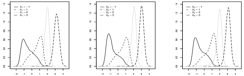
Figure 3: Posterior distributions for $\delta_{1}$, $\delta_{2}$ and $\delta_{3}$ under four simulated data sets in Case A. The legends indicate the values of $\delta_{i}$’s used to generate data sets.

Our results are based on a MCMC chain of length 500000 with a burn-in of 100000, using the block MCMC algorithm in Section 5. Figure 3 displays the posterior distributions for $\delta_{1}$, $\delta_{2}$ and $\delta_{3}$ under four data sets introduced in Case A. These figures clearly indicate that the data allow for meaningful inference on ${\boldsymbol{\delta}}$ since the posterior distributions assign a large mass to neighborhoods of the values used to generate the data, specially for larger values of the skewness. Figure 4 displays the posterior inference for $L_{12}$ and $L_{23}$ under four data sets in Case B. Figure 5 displays the posterior distributions for (left figure) $\delta_{1}$, $\delta_{2}$, $\delta_{3}$ and (right figure) $L_{12}$ and $L_{23}$ under a data set introduced in Case C which indicates the data clearly allows for good inference.

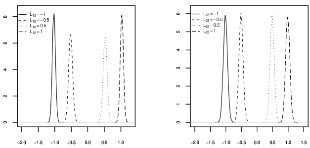
Figure 4: Posterior distributions for $L_{12}$ and $L_{23}$ under four simulated data sets in Case B. The legends indicate the values of $L_{12}$ and $L_{23}$ used to generate the data sets.

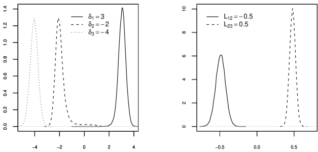
Figure 5: Posterior distributions for (left figure) $\delta_{1}$, $\delta_{2}$, $\delta_{3}$ and (right figure) $L_{12}$ and $L_{23}$ under simulated data in Case C. The legends indicate the values of these parameters used to generate the data.

6 Case studies

In this section, we apply our approach to two data sets: student’s mathematics marks from Mardia et al. (1979) and the carcass data from Busk et al. (1999). We compare the results with those obtained from the Gaussian model. Our results are based on a MCMC chain of length 700000 with a burn-in 200000. All results in this section were computed under prior (11) with $b_{1}=100$, ${\boldsymbol{\mu}}_{0}={\bf 0}$, $b_{2}=10^{4}$, $b_{3}=b_{4}=10^{-6}$ and $b_{5}=100$ which gives us a diffuse prior.

6.1 Mathematics Marks

Table 2: The sample partial correlation matrix of the mathematics marks.

	Mechanics	Vectors	Algebra	Analysis	Statistics
Mechanics	1	0.33	0.23	0.00	0.02
Vectors		1	0.28	0.08	0.02
Algebra			1	0.43	0.36
Analysis				1	0.25
Statistics					1

This data set come from Mardia et al. (1979), and consists of examination marks of 88 students in the five subjects mechanics, vectors, algebra, analysis and statistics. Mechanics and vectors were closed book examinations and the reminder were open book. All variables are measured on the same scale (0-100). Table 2 displays sample partial correlation matrix between these variables. The element in the upper righthand block are all near zero which it means that we can consider mechanics and analysis conditionally independent on the other remaining variables, as are mechanics and statistics, vectors and statistics and finally vectors and analysis. These assumptions have been described in neighborhood graph in Figure 6 as suggested by Whittaker (1990). For exploratory purpose, the histograms of variables are plotted in Figure 7. These histograms suggest that analysis and statistics marks have skewed distributions in left and right, respectively. We used the following ordering for our analysis: $\{$Mechanics, Vectors, Algebra, Analysis, Statistics$\}$.

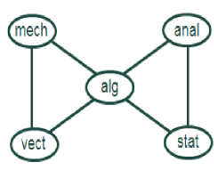
Figure 6: Neighborhood graph of mathematics marks.

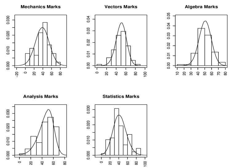
Figure 7: Histograms of mathematics marks and fitted models to those.

The posterior mean (standard deviation) estimates of nonzero elements of upper triangular matrix $L$ under GG and SGDG model are as follows

$$\scriptsize\hat{L}_{GG} = \left(\begin{array}[]{ccccc}1&-0.46_{(0.15)}&-0.55_{(0.18)}&0.00&0.00\\ &1&-0.75_{(0.11)}&0.00&0.00\\ &&1&-0.35_{(0.06)}&-0.23_{(0.05)}\\ &&&1&-0.52_{(0.07)}\\ &&&&1\\ \end{array}\right),$$

$$\scriptsize\hat{L}_{SGDG} = \left(\begin{array}[]{ccccc}1&-0.46_{(0.14)}&-0.55_{(0.17)}&0.00&0.00\\ &1&-0.76_{(0.09)}&0.00&0.00\\ &&1&-0.32_{(0.06)}&-0.24_{(0.05)}\\ &&&1&-0.44_{(0.05)}\\ &&&&1\\ \end{array}\right).$$

The posterior mean estimates of the other parameters is shown in Table 3. Recall that $\delta_{i}$ is not skewness parameter of $i$th variable only, but the $\delta_{i}$’s in Table 3 can be approximately interpreted as skewness parameters of the rows of $\hat{L}_{SGDG}X$ where $X$=(Mechanics, Vectors, Algebra, Analysis, Statistics). Figure 7 shows the histograms of variables with the fitted SGDG model. The fits seems adequate.

To compare the GG and SGDG model, we computed the Bayes factor using the modified harmonic mean estimator $\hat{p}_{4}$ of Newton and Raftery (1994). The Bayes factor in favor of the SGDG model is $3\times 10^{37}$, which indicates overwhelming support for the SGDG model. We also tried other vertex-orderings corresponding to a perfect vertex elimination scheme, but the chosen ordering in the first of this section (i.e. $\{$Mechanics, Vectors, Algebra, Analysis, Statistics$\}$) was supported by the Bayes factor. Additionally, note that although the SGDG model depends on the ordering of the vertices, it give a better fit in compare with the corresponding GG model over all vertex-orderings corresponding to a perfect vertex elimination scheme.

Table 3: Mathematics marks: Posterior means (standard deviation) for parameters.

		SGDG		GG
i
	${\boldsymbol{\beta}}$	${\boldsymbol{\omega}}^{2}$	${\boldsymbol{\delta}}$	${\boldsymbol{\beta}}$	${\boldsymbol{\omega}}^{2}$
1	$45.83_{(5.75)}$	$0.0057_{(0.0015)}$	$0.38_{(6.15)}$	$39.16_{(1.83)}$	$0.0051_{(0.0008)}$
2	$61.21_{(4.83)}$	$0.0235_{(0.0174)}$	$-9.17_{(5.63)}$	$50.68_{(1.44)}$	$0.0091_{(0.0014)}$
3	$55.18_{(3.27)}$	$0.0469_{(0.0279)}$	$-5.51_{(4.15)}$	$50.64_{(1.12)}$	$0.0211_{(0.0032)}$
4	$56.17_{(2.30)}$	$0.2131_{(0.3696)}$	$-18.29_{(1.88)}$	$46.77_{(1.56)}$	$0.0071_{(0.0011)}$
5	$30.53_{(3.68)}$	$0.0065_{(0.0025)}$	$14.54_{(3.89)}$	$42.25_{(1.88)}$	$0.0034_{(0.0005)}$

6.2 Carcass Data

The carcass data from gRbase package of R contains measurements of the thickness of meat and fat layers together with the lean meat percentage of 344 slaughter carcasses at three Danish slaughter houses. Seven variables has been defined in this data set as follows:

• F11, F12, F13: Thickness of fat layer at 3 different locations on the back of the carcass.

• M11, M12, M13: Thickness of meat layer at 3 different locations on the back of the carcass.

• LMP: Lean meat percentage determined by dissection

This data set has been used for estimating the parameters in a prediction formula for prediction of lean meat percentage on the basis of the thickness measurements on the carcass. Data are described in detail in Busk et al. (1999). Hojsgaard et al. (2012) provided some neighborhood graphs for these variables in term of different model selection methods. Based on the BIC criterion, they proposed the neighborhood graph in Figure 8.

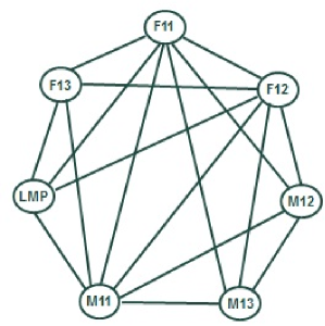
Figure 8: Neighborhood graph of carcass data.

Table 4: Carcass Data: Posterior means (standard deviation) for parameters.

		SGDG		GG
i
	${\boldsymbol{\beta}}$	${\boldsymbol{\omega}}^{2}$	${\boldsymbol{\delta}}$	${\boldsymbol{\beta}}$	${\boldsymbol{\omega}}^{2}$
1	$51.67_{(2.62)}$	$0.152_{(1.41)}$	$0.54_{(0.025)}$	$52.01_{(0.41)}$	$0.133_{(0.010)}$
2	$55.89_{(2.38)}$	$0.112_{(1.70)}$	$0.87_{(0.021)}$	$55.70_{(0.35)}$	$0.096_{(0.007)}$
3	$52.44_{(2.15)}$	$0.047_{(2.46)}$	$1.32_{(0.008)}$	$51.98_{(0.31)}$	$0.041_{(0.003)}$
4	$63.81_{(0.96)}$	$0.326_{(0.91)}$	$-2.06_{(0.085)}$	$59.38_{(0.19)}$	$0.196_{(0.015)}$
5	$10.24_{(0.83)}$	$0.615_{(0.79)}$	$0.43_{(0.131)}$	$12.95_{(0.15)}$	$0.510_{(0.038)}$
6	$13.46_{(0.98)}$	$0.342_{(1.06)}$	$0.25_{(0.062)}$	$16.49_{(0.18)}$	$0.293_{(0.023)}$
7	$10.96_{(0.54)}$	$0.286_{(0.66)}$	$3.75_{(0.090)}$	$13.96_{(0.16)}$	$0.112_{(0.009)}$

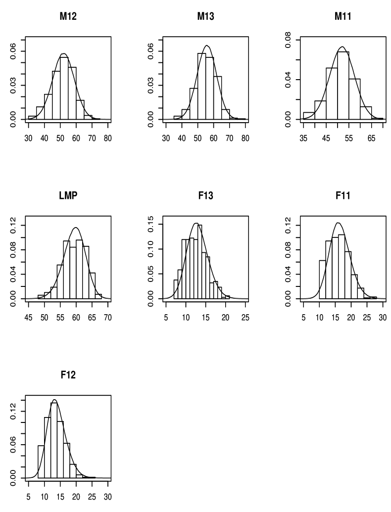
Figure 9: Histograms of carcass data and fitted models to those.

We used first the ordering: $\{M12,M13,M11,LMP,$ $F13,F11,F12\}$. A summary of the posterior inference on the parameters in the models is provided in Table 4. We also present two quantities that are directly comparable between the SGDG and GG model. In Figure 9, we have displayed the fitted SGDG model to this data set. The SGDG model seems to fit well and includes skewness for LMP, F13, F11 and F12. The Bayes factor in favor of the SGDG versus the GG model was estimated to $1.7\times 10^{8}$. We also tried an alternative orderings for our analysis, but they gave all a worse fit.

7 Conclusions

In this paper, we have proposed a novel decomposable graphical model to accommodate skew-Gaussian decomposable graphical model (SGDG). The SGDG model reflect conditional independencies among the components of the multivariate closed skew normal random vector with respect to a decomposable graph, and includes the Gaussian graphical models as a particular case.

We develop a family of conjugate prior distributions for precision matrix, and derive a condition which ensures propriety of the posterior distribution corresponding to the standard noninformative priors for mean vector, precision parameters and lower triangular matrix as well as proper prior for skewness parameter.We successfully apply our new model to two data sets, showing great improvement on the Gaussian graphical model.

Since the SGDG model satisfy the conditional independence property only under a decomposable graph, so an extension of the SGDG model for other graphs requires further research.

APPENDIX: PROOFS

To prove Theorem 1, we use the following factorization criterion.

Lemma 4: Two random variables $X$ and $Y$ are called conditionally independent given $Z$ iff there exist some functions $f$ and $g$ such that $\pi(x,y,z)=f(x,z)g(y,z)$ (see Rue and Held (2005)).

Proof of Theorem 1: We partition ${\bf X}$ as $(X_{i},X_{j},{\bf X}_{-ij})$ and then use the multivariate version of the factorization criterion on $\pi(x_{i},x_{j},{\bf x}_{-ij})$. Fix $i\neq j$ and assume $\boldsymbol{\mu}={\bf 0}$ without loss of generality. From (8) we get

$$\pi(x_{i},x_{j},{\bf x}_{-ij})\propto\exp(-\frac{1}{2}\sum_{m,l}x_{m}\ Q_{ml}\ x_{l})\prod_{r=1}^{k}\ \Phi_{1}(\alpha_{r}\kappa_{r}L_{r.}^{\prime}{\bf x};\ 0,\ 1),$$

where $\kappa_{r}$ is root square of the $r$’th diagonal element of $D_{\kappa}$ and $L_{r.}$ is $r$’th row of $L$. Let $i<j$ without loss of generality. Now, we define set

$$I = \{r:\ \ L_{ri}\neq 0\ \ and\ \ L_{rj}=0\ \ for\ \ r\leq i\}$$

Then, due to the ordering of the vertices corresponds to a perfect vertex elimination scheme and with respect to Definition 2, we know if $\upsilon<i<j$ then the neighbors of vertex $\upsilon$ can not be vertex $i$ and $j$ together if and only if vertices $i$ and $j$ are not neighbors. Hence, we have

$$\pi(x_{i},x_{j},{\bf x}_{-ij}) \propto \exp(-\frac{1}{2}x_{i}x_{j}(Q_{ij}+Q_{ji})-\frac{1}{2}\sum_{\{m,l\}\neq\{i,j\}}x_{m}\ Q_{ml}\ x_{l})$$

$$\times \prod_{r\in I}\ \Phi_{1}(\alpha_{r}\kappa_{r}L_{r.}^{\prime}{\bf x};\ 0,\ 1)\prod_{r\notin I}\ \Phi_{1}(\alpha_{r}\kappa_{r}L_{r.}^{\prime}{\bf x};\ 0,\ 1).$$

Second term does not involve $x_{i}x_{j}$ while first term involves $x_{i}x_{j}$ iff $Q_{ij}\neq 0$. Thus, one example for functions $f$ and $g$ in lemma can be defined as

$$f(x_{i},{\bf x}_{-ij}) = \exp(-\frac{1}{2}\sum_{\{m,l\}\neq j}x_{m}\ Q_{ml}\ x_{l})\prod_{r\in I}\ \Phi_{1}(\alpha_{r}\kappa_{r}L_{r.}^{\prime}{\bf x};\ 0,\ 1)$$

$$g(x_{j},{\bf x}_{-ij}) = \exp(-\frac{1}{2}\sum_{\{m,l\}\neq i}x_{m}\ Q_{ml}\ x_{l})\prod_{r\notin I}\ \Phi_{1}(\alpha_{r}\kappa_{r}L_{r.}^{\prime}{\bf x};\ 0,\ 1).$$

iff $Q_{ij}\neq 0$. The claim then follows. $\blacksquare$.

Proof of Theorem 2: At first, we recall if $G$ be a nondecomposable undirected graph, then it is possible that the zero elements of precision matrix $Q$ are not reflected in its modified cholesky decomposition $L$. To prove this theorem, we proceed similar to Theorem 1. Fix $i<j$ and assume $\boldsymbol{\mu}={\bf 0}$ without loss of generality. Here, we know when $F(i,j)$ separates vertices $i$ and $j$, then $L_{ij}=0$ and it is not possible to have a pass from $i$ to $j$ with passing from some vertex that the number of all of them are smaller than $i$. Thus, if $\upsilon<i<j$, then $\upsilon$ can not be the neighbors of vertex $i$ and $j$ together. Hence, we can write $\pi(x_{i},x_{j},{\bf x}_{-ij})$ similar to (7) with same definition for set $I$. The rest of the proof is similar to that of Theorem 1.  $\blacksquare$

Proof of Theorem 3: At first, we denote $L_{i\cdot}$ as $i$’th row of $L$. Now, we have

$$\int\prod_{i=1}^{k}(\omega^{2}_{i})^{\psi_{i}/2-1}\exp\{-\frac{1}{2}tr((L^{\prime}D_{\omega}L)\Psi)\}dDdL$$

$$= \int\prod_{i=1}^{k}(\omega^{2}_{i})^{\psi_{i}/2-1}\exp\{-\frac{1}{2}(L\Psi L^{\prime})_{ii}\omega^{2}_{i}\}dDdL\propto\int\prod_{i=1}^{k}\frac{1}{(L\Psi L^{\prime})_{ii}^{\psi_{i}/2}}dL$$

$$\propto \prod_{i=1}^{k-1}\int\frac{1}{(L_{i\cdot}\Psi L_{i\cdot}^{\prime})^{\psi_{i}/2}}dL_{i\cdot}=\prod_{i=1}^{k-1}\int_{\Re^{||N^{\prec}(i)||}}\frac{1}{(L_{i\cdot}^{*}\Psi^{(i)}L_{i\cdot}^{*^{\prime}})^{\psi_{i}/2}}dL_{i\cdot}^{\neq 0}$$

where $L_{i\cdot}^{*}=(1\ \ L_{i\cdot}^{\neq 0})^{\prime}$. Also, $\Psi^{(i)}$ is a submatrix of $\Psi$ corresponding to the elements of $L_{i\cdot}^{*}$. We are now in the same line with Khare and Rajaratnam (2011) and similarly, we can show that the integral is finite if $\psi_{i}>||N^{\prec}(i)||$.  $\blacksquare$

Proof of Theorem 4: Under the introduced reparemeterizations in hierarchical model (10), the conditional density of ${\bf X}$ becomes

$$p({\bf x}|{\boldsymbol{\mu}},{\boldsymbol{\omega}}^{2},{\boldsymbol{\delta}},L)=(\frac{2}{\pi})^{k/2}|D_{g}|^{\frac{1}{2}}e^{-\frac{1}{2}({\bf x}-{\boldsymbol{\mu}})^{\prime}Q_{g}({\bf x}-{\boldsymbol{\mu}})}\prod_{i=1}^{k}\Phi(\delta_{i}\omega_{i}\sqrt{g(\omega_{i},\delta_{i})}L({\bf x}-{\boldsymbol{\mu}});0,1),$$

where $g(\omega_{i},\delta_{i})=\frac{\omega^{2}_{i}}{1+\delta_{i}^{2}\omega^{2}_{i}}$, $D_{g}=diag(g(\omega_{1},\delta_{1})),\cdots,g(\omega_{k},\delta_{k})$ and $Q_{g}=L^{\prime}D_{g}L$. Now, since $0\leq\Phi(\cdot)\leq 1$, we have

$$p({\bf x}) = \int_{\Re^{N}}\int_{\Re^{k}}\int_{\Re_{+}^{k}}\int_{\Re^{k}}p({\bf x}|{\boldsymbol{\mu}},{\boldsymbol{\omega}}^{2},{\boldsymbol{\delta}},L)\pi({\boldsymbol{\mu}})\pi({\boldsymbol{\delta}}|{\boldsymbol{\omega}}^{2})\pi(L,D_{\omega})d{\boldsymbol{\mu}}d{\boldsymbol{\omega}}^{2}d{\boldsymbol{\delta}}dL$$

$$< \int_{\Re^{N}}\int_{\Re^{k}}\int_{\Re_{+}^{k}}\int_{\Re^{k}}|D_{g}|^{\frac{n}{2}}e^{-\frac{1}{2}\sum_{i=1}^{n}({\bf x}_{i}-{\boldsymbol{\mu}})^{\prime}Q_{g}({\bf x}-{\boldsymbol{\mu}}_{i})}\pi({\boldsymbol{\delta}}|{\boldsymbol{\omega}}^{2})\pi(L,D_{\omega})d{\boldsymbol{\mu}}d{\boldsymbol{\omega}}^{2}d{\boldsymbol{\delta}}dL$$

$$= K_{1}\int_{\Re^{k}}f_{N}^{k}(\boldsymbol{\mu}|\bar{\bf x},(nQ_{g})^{-1})d{\boldsymbol{\mu}}$$

$$\times \int_{\Re^{N}}\int_{\Re^{k}}\int_{\Re_{+}^{k}}|D_{g}|^{\frac{n}{2}}|Q_{g}|^{-\frac{1}{2}}e^{-\frac{1}{2}\sum_{i=1}^{n}({\bf x}_{i}-\bar{\bf x})^{\prime}Q_{g}({\bf x}_{i}-\bar{\bf x})}\pi({\boldsymbol{\delta}}|{\boldsymbol{\omega}}^{2})\pi(L,D_{\omega})d{\boldsymbol{\omega}}^{2}d{\boldsymbol{\delta}}dL$$

where $N=\sum_{i=1}^{k-1}||N^{\prec}(i)||$, $\bar{\bf x}=\frac{1}{n}\sum_{i=1}^{n}{\bf x}_{i}$ and $K_{1}$ is a constant. If we define $S=\sum_{i=1}^{n}({\bf x}_{i}-\bar{\bf x})({\bf x}_{i}-\bar{\bf x})^{\prime}$ and using variable transformation ${\lambda}_{i}=\delta_{i}{\omega}_{i}$, $i=1,\cdots,k$, under $n\geq 2$, we get

$$p({\bf x}) < K_{2}\int_{\Re^{N}}\int_{\Re^{k}}\int_{\Re_{+}^{k}}\prod_{i=1}^{k}(\frac{1}{1+\delta_{i}^{2}\omega^{2}_{i}})^{\frac{n-1}{2}}\prod_{i=1}^{k}(\omega^{2}_{i})^{\frac{n}{2}-1}e^{-\frac{1}{2}tr(Q_{g}S)}e^{-\frac{1}{2b_{2}}\sum_{i=1}^{k}\omega^{2}_{i}\delta_{i}^{2}}d{\boldsymbol{\omega}}^{2}d{\boldsymbol{\delta}}dL$$

$$= K_{2}\int_{\Re^{N}}\int_{\Re^{k}}\int_{\Re_{+}^{k}}\prod_{i=1}^{k}\{(\frac{1}{1+\lambda_{i}^{2}})^{\frac{n-1}{2}}e^{-\frac{1}{2b_{2}}\lambda_{i}^{2}}(\omega^{2}_{i})^{\frac{n-1}{2}-1}e^{-\frac{1}{2}\frac{(LSL^{\prime})_{ii}}{1+\lambda_{i}^{2}}\omega^{2}_{i}}\}d{\boldsymbol{\omega}}^{2}d{\boldsymbol{\lambda}}dL$$

$$\propto K_{2}\int_{\Re^{N}}\prod_{i=1}^{k}\frac{1}{(LSL^{\prime})_{ii}^{\frac{n-1}{2}}}dL=\prod_{i=1}^{k-1}\int_{\Re^{||N^{\prec}(i)||}}\frac{1}{(L_{i\cdot}^{*}\Psi^{(i)}L_{i\cdot}^{*^{\prime}})^{\frac{n-1}{2}}}dL_{i\cdot}^{\neq 0}$$

where $K_{2}$ is another constant. Similarly to the proof of Theorem 3, we can show that the integral is finite if $n\geq\max\{||N^{\prec}(i)||\}+2$.  $\blacksquare$

References

- [1] Allard, D., Naveau, P. 2007. A new spatial skew-normal random field model. Communications in Statistics 36, 1821-1834.
- [2] Azzalini, A. 2005. The skew-normal distribution and related multivariate families. Scandinavian Journal of Statistics 32, 159-188.
- [3] Azzalini, A., Capitanio, A. 1999. Statistical applications of the multivariate skew normal distribution. Journal of the Royal Statistical Association 61, 579-602.
- [4] Busk, H., Olsen, E.V., Brondum, J. 1999. Determination of lean meat in pig carcasses with the Autofom classification system. Meat Science 52, 307-314.
- [5] Capitanio, A., Azzalini, A., Stanghellini, E. 2003. Graphical models for skew-normal variates. Scandinavian Journal of Statistics 30, 129-144.
- [6] Dominguez-Molina, J., Gonzalez-Farias, G., Gupta, A.K. 2003. The multivariate closed skew-normal distribution. Technical Report 03-12. Department of Mathematics and Statistics, Bowling Green State University.
- [7] Florens, J.P., Mouchart, M., Rolin, J.M. 1990. Invariance arguments in Bayesian statistics. In Economic Decision Making: Games, Econometrics and Optimisation (eds. J. Gabszewicz, J.F. Richard and L.A. Wolsey). Amsterdam: North-Holland.
- [8] Giudici, P., Green, P. 1999. Decomposable graphical Gaussian model determination. Biometrika 86, 785-801.
- [9] Gonzalez-Farias, G., Dominguez-Molina, J., Gupta, A. 2004. The closed skew-normal distribution. In: Genton, M., ed. Skew-Elliptical Distributions and Their Applications: A Journey Beyond Normality. Boca Raton, FL: Chapman Hall/CRC, 25-42.
- [10] Hojsgaard, S., Edwards, D., Lauritzen, S. 2012. Graphical models with R. Springer-Verlag, New York.
- [11] Khare, K., Rajaratnam, B. 2011. Wishart distributions for decomposable covariance graph models. Annals of Statistics 39, 514 555.
- [12] Lauritzen, S.L. 1996. Graphical models. Oxford University Press, New York.
- [13] Letac, G., Massam, H. 2007. Wishart distributions for decomposable graphs. Annals of Statistics 35, 1278-1323.
- [14] Mardia, K.V., Kent, J.T., Bibby, J.M. 1979. Multivariate analysis, New York: Academic Press.
- [15] Mouchart, M. 1976. A note on Bayes theorem. Statistica 36, 349-357.
- [16] Newton, M.A., Raftery, A.E. 1994. Approximate Bayesian inference by the weighted likelihood bootstrap(with discussion). Journal of the Royal Statistical Association 3, 3-48.
- [17] Paulsen, V.I., Power, S.C., Smith, R.R. 1989. Schur products and matrix completions. Journal of Functional Analysis 85, 151-178.
- [18] Rue, H., Held, L. 2005. Gaussian Markov random fields: Theory and Applications. London: Chapman and Hall CRC Press.
- [19] Whittaker, J. 1990. Graphical models in applied multivariate statistics. Wiley, Chichester.