Online partial evaluation of sheet-defined functions

Abstract

We present a spreadsheet implementation, extended with sheet-defined functions, that allows users to define functions using only standard spreadsheet concepts such as cells, formulas and references, requiring no new syntax. This implements an idea proposed by Peyton-Jones and others [14].

As the main contribution of this paper, we then show how to add an online partial evaluator for such sheet-defined functions. The result is a higher-order functional language that is dynamically typed, in keeping with spreadsheet traditions, and an interactive platform for function definition and function specialization.

We describe an implementation of these ideas, present some performance data from microbenchmarks, and outline desirable improvements and extensions.

1 Introduction

Spreadsheet programs such as Microsoft Excel, OpenOffice Calc and Gnumeric provide a simple, powerful and easily mastered end-user programming platform for mostly-numeric computation. Yet as observed by several authors [13, 14], spreadsheets lack the most basic abstraction mechanism: The ability to create a named function directly from spreadsheet formulas.

Although most spreadsheet programs allow function definitions in external languages such as VBA, Java or Python, those languages have a completely different programming model that many competent spreadsheet users find impossible to master. Moreover, the external language bindings are sometimes surprisingly inefficient.

Here we present an implementation of sheet-defined functions in the style Nuñez [13] and Peyton-Jones et al. [14] that (1) uses only standard spreadsheet concepts and notations, no external languages, so it should be understandable to competent spreadsheet users, and (2) is very efficient, so that user-defined functions can be as fast as built-in ones. The ability to define functions directly from spreadsheet formulas should (3) encourage the development of shared function libraries, which in turn should (4) improve reuse, reliability and upgradability of spreadsheet models.

Moreover, we believe that partial evaluation, or automatic program specialization, is a plausible tool in the declarative and interactive context of spreadsheets. In particular, the specialization of a function closure fv is achieved through a simple function call SPECIALIZE(fv), which creates a new specialized function and returns a closure for it. The resulting specialized function can be invoked immediately and is used exactly like the given unspecialized one; but (hopefully) executes faster. No external files are created and no compilers need to be invoked. The design and implementation of this idea are the main contributions of this paper, presented in sections 6 through 8.

Our motivation is pragmatic. A sizable minority of spreadsheet users, including biologists, physicists and financial analysts, build very complex spreadsheet models. This is because it is convenient to experiment with both models and data, and because the models are easy to share and distribute. We believe that one can advance the state of the art by giving spreadsheet users better tools, rather than telling them that they should have used Matlab, Java, Python or Haskell instead.

Another paper, describing complementary aspects of this work, in particular details of evaluation conditions as well as a case study on implementing financial functions, appears elsewhere [20]; section 2 of the present paper is reproduced from that paper. Many more technical details are given in a draft technical report [19]. Our prototype source code is available from http://www.itu.dk/people/sestoft/funcalc/.

2 Sheet-Defined Functions

We first give two motivating examples of sheet-defined functions.

Example 2.1.

Consider the problem of calculating the area of each of a large number of triangles whose side lengths $a$, $b$ and $c$ are given in columns E, F and G of a spreadsheet, as in Figure 1. The area can be computed by the formula $\sqrt{s(s-a)(s-b)(s-c)}$ where $s=(a+b+c)/2$ is half the perimeter. Now, either one must allocate a column H to hold the value $s$ and compute the area in column I, or one must inline $s$ four times in the area formula. The former pollutes the spreadsheet with intermediate results, whereas the latter would create a long expression that is nearly impossible to enter without mistakes. It is clear that many realistic problems would require even more space for intermediate results and even more unwieldy formulas.

Here we propose instead to define a function, TRIAREA say, using standard spreadsheet cells and formulas, but on a separate function sheet, and then call this function as needed from the sheet containing the triangle data.

Figure 2 shows a function sheet containing a definition of function TRIAREA, with inputs $a$, $b$ and $c$ in cells A3, B3 and C3, the intermediate result $s$ in cell D3, and the output in cell E3.

Figure 3 shows an ordinary sheet with triangle side lengths in columns E, F and G, and function calls =TRIAREA(E2,F2,G2) in column H to compute the triangles’ areas. There are no intermediate results; these exist only on the function sheet. As usual in spreadsheets, it suffices to enter the function call once in cell H2 and then copy it down column H with automatic adjustment of cell references.

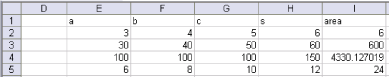
Figure 1: Triangle side lengths and computed areas, with intermediate results in column H.

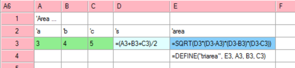
Figure 2: Function sheet, where DEFINE in E4 creates function TRIAREA with input cells A3, B3 and C3, output cell E3, and intermediate cell D3.

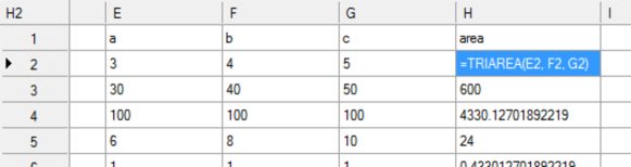
Figure 3: Ordinary sheet calling TRIAREA, defined in Figure 2, from cells H2:H5.

Example 2.2.

Microsoft Excel has a built-in function REPT($s$,$n$) that computes $s^{n}$, the string consisting of $n\geq 0$ concatenated copies of string $s$. This built-in function can be implemented efficiently as a recursive sheet-defined function REPT4(s,n) as shown in figure 4. This implementation is optimal, using $O(\log n)$ string concatenation operations, written (&), for a total running time of $O(n\cdot|s|)$, where $|s|$ is the length of $s$.

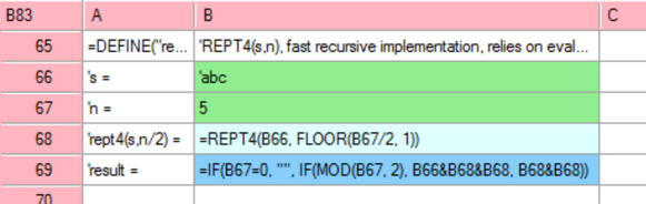
Figure 4: Recursive function REPT4(s,n) computes $s^{n}$, the concatenation of $n$ copies of string $s$. Cells B66 and B67 are input cells, B69 is the output cell, and B68 holds an intermediate result.

In contrast to Peyton-Jones et al., we allow sheet-defined functions to be recursively defined, because that is necessary to reimplement many built-in functions, and higher-order, because that generalizes many of Excel’s ad hoc functions (such as SUMIF, COUNTIF) and features (such as Goal Seek).

3 Dual implementation: Interpretation and compilation

Our spreadsheet implementation, called Funcalc, is written in C# and consists of an interpretive implementation of ordinary sheets, described in this section, and a compiled implementation of sheet-defined functions, described in section 4. The rationale for having both is that ordinary sheets will be edited frequently but each cell’s formula is evaluated only once every recalculation, whereas a sheet-defined function will be edited rarely but may be called thousands of times in every recalculation. Hence compilation would cause much overhead and provide little benefit in ordinary sheets, but causes little overhead and provides much benefit in function sheets.

Funcalc uses the standard notions of workbook, worksheet, cell, formula and built-in function. A cell may contain a constant or a formula (or nothing); a formula in a cell consists of an expression and a cache for the expression’s value.

3.1 Interpretive implementation

The interpretive implementation is used to evaluate formulas on ordinary sheets. Spreadsheet formulas are dynamically typed, so runtime values are tagged by runtime types such as Number, Text, Error, Array, and Function, with common supertype Value. Such tagged runtime values will generally be allocated as objects in the garbage-collected heap.

A formula expression e in a given cell on a given worksheet is evaluated interpretively by calling e.Eval(sheet,col,row), which returns a Value object. A simple interpretive evaluator guided by the expression abstract syntax tree will involve wrapping of result values upon return, followed by unwrapping when the value is used. This overhead is especially noticeable when a 64-bit floating-point number (type double, which could be stack-allocated) gets wrapped as a heap-allocated Number object. An important goal of the compiled implementation (section 4) is to avoid this overhead.

A technical report [19] gives more details about the interpretive implementation and its design tradeoffs.

4 Compiled implementation of sheet-defined functions

The compiled implementation is used to execute sheet-defined functions.

4.1 Defining functions and creating closures

We add just three new built-in functions to support the definition and use of sheet-defined functions, including higher-order ones. There is a function to define a new sheet-defined function:

• DEFINE("name", out, in1..inN) creates a function with the given name, result cell out, and input cells in1..inN, where N >= 0, as shown in figure 2 cell E4.

Two other functions are used to create a function value (closure) and to apply it, respectively:

• CLOSURE("name", e1..eM) evaluates argument expressions e1..eM to values a1..aM and returns a closure for the sheet-defined function "name". An argument ai that is an ordinary value gets stored in the closure, whereas an argument that is #NA, for “not available”, signifies that this argument must be provided later when calling the closure.

• APPLY(fv, e1..eN) evaluates fv to a closure, evaluates argument expressions e1..eN to values b1..bN, and applies the closure by using the bj values for those arguments in the closure that were #NA at closure creation.

The #NA mechanism provides a very flexible way to create closures, or partially applied functions. For instance, given a function MONTHLEN(y,m) to compute the number of days in month m of year y, we may create the closure CLOSURE("MONTHLEN", 2013, #NA) which computes the number of days in any month in 2013, or we may create the closure CLOSURE("MONTHLEN", #NA, 2) which computes the number of days in February in any year. This notational flexibility is rather unusual from a programming language perspective, but fits well with the standard spreadsheet usage of #NA to denote a value that is not (yet) available.

The built-in functions DEFINE, CLOSURE and APPLY provide the general computation model for higher-order functions in our implementation, and are the only means needed to define functions, create closures, and call closures. See also figure 7. All the required syntax is already present in standard spreadsheet implementations.

Section 6 shows that these functions fit excellently with the single new function SPECIALIZE needed to partially evaluate closures.

4.2 Overall compilation process

The compiled implementation of sheet-defined functions generates CLI (.NET) bytecode at runtime. Runtime bytecode generation maintains the interactive style of spreadsheet development and some portability, while achieving good performance because the .NET just-in-time compiler turns the bytecode into efficient machine code.

The compilation of a sheet-defined function proceeds in these steps:

1. Build a dependency graph of the cells transitively reachable, by cell references, from the output cell.

2. Perform a topological sort of the dependency graph, so a cell is preceded by all cells that it references. It is illegal for a sheet-defined function to have static cyclic dependencies.

3. If a cell in the graph is referred only once (statically), inline its formula at its unique occurrence. This saves a local variable at no cost in code size or computation time.

4. Using the dependency graph, determine the evaluation condition [20] for each cell; build a new dependency graph that takes evaluation conditions into account; and redo the topological sort. The result is a list of ComputeCell objects, each containing a cell c and an associated variable v_c.

5. Generate CLI bytecode: traverse the list in forward topological order, and for each pair of a cell c and associated variable v_c, generate code for the assignment v_c = <code for c’s formula>.

The evaluation conditions mentioned in step 4 are needed to correctly evaluate recursive functions such as that in example 2.2; see [20] for more details.

The formula in a cell c contains an expression represented by abstract syntax of type CGExpr (for code generating expression); see figure 5.

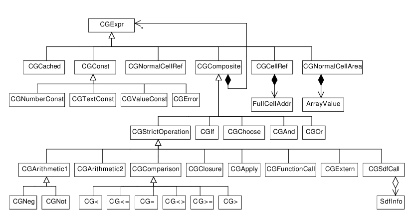
Figure 5: Class diagram for Funcalc’s expression abstract syntax. All expressions are side effect free except possibly calls to external functions (CGExtern). The rather elaborate inheritance structure facilitates ordinary code generation as well as partial evaluation. A CGClosure is a CLOSURE() call, CGApply is an APPLY() call, CGFunctionCall is a call to any other built-in function, CGExtern is a call to an external .NET function, and CGSdfCall is a call to a sheet-defined function. This is used in section 7.

4.3 Context-dependent compilation

This section describes the compilation, basically step 5 in section 4.2, of a formula expression represented by the abstract syntax shown in figure 5. Compilation to CLI bytecode is performed at runtime by a straightforward recursive traversal of the abstract syntax tree [18]. The main embellishments of the code generation serve (1) to avoid wrapping 64-bit floating-point numbers as heap-allocated Number objects, (2) to represent and propagate error values efficiently, and (3) to implement proper tail recursion for sheet-defined functions. Point (2) is required by spreadsheet semantics: a failed computation must produce an error value, and such error values must propagate from operands to results in any context, such as arithmetics, comparisons, conditions, and function calls.

Achieving (3) is near-trivial, using the CLI “tail.” instruction prefix (as in example 8.4); how to achieve (1) and (2) is described in the remainder of this section.

4.3.1 No value wrapping

The simplest compilation scheme, implemented by the method Compile on expressions, generates code to emulate interpretive evaluation. The call e.Compile() must generate code that, when executed, leaves the value of e on the stack top as a Value object.

However, using Compile would wrap every intermediate result as an object of a subclass of Value, which would be inefficient, in particular for numeric operations. In an expression such as A1*B1+C1, the intermediate result A1*B1 would be wrapped as a Number object, only to be immediately unwrapped before the addition. The creation of that Number object would dominate all other costs, because it requires allocation in the heap and causes work for the garbage collector.

To avoid runtime wrapping of results that will definitely be used as numbers, we introduce another compilation method. The call e.CompileToDoubleOrNan() must generate code that, when executed, leaves the value of e on the stack as a 64-bit floating-point value. If the result is an error value, then the number will be a NaN.

4.3.2 Error propagation

When computing with naked 64-bit floating-point values, we represent an error value as a NaN and use the 51 bit “payload” of the NaN to distinguish error values, as per the ieee754 standard [9, section 6.2]. Since arithmetic operations and mathematical functions preserve NaN operands, we get error propagation for free. For instance, if d is a NaN, then Math.Sqrt(6.1*d+7.5) will be a NaN with the same payload, thus representing the same error. As an alternative to error propagation via NaNs, one could use CLI exceptions, but these turn out to be several orders of magnitude slower. This inefficiency matters little in well-written C# software, which should not use exceptions for control flow, so a single exception would terminate the software. By contrast, a spreadsheet workbook may have thousands of cells that have error values during workbook editing, and these may be reevaluated whenever a single cell has been edited.

If both d1 and d2 are NaNs, then by the ieee754 standard d1+d2 must be a NaN with the same payload as one of d1 and d2. Hence at most one error can be propagated at a time, but that fits well with spreadsheet development: The user fixes one error, only to see another error appear, then fixes that one, and so on.

4.3.3 Compilation of comparisons

According to spreadsheet principles, comparisons such as B8>37 must propagate errors, so that if B8 evaluates to an error, then the comparison evaluates to the same error. When compiling a comparison we cannot rely on NaN propagation; a comparison involving one or more NaNs is either true or false, not undefined, in CLI [5, section III.3]. Hence we introduce yet another compilation method on expressions.

The call e.CompileToDoubleProper(ifProper,ifBad) must generate code that evaluates e; and if the value is a non-NaN number, leaves it on the stack top as a 64-bit floating-point value and continues with the code generated by ifProper; else, it leaves the value in a special variable and continues with the code generated by ifBad.

Here ifProper and ifBad are themselves code generators, which generate the success continuation and the failure continuation [21] of the evaluation of e.

The default implementation of e.CompileToDoubleProper uses e.CompileToDouble to generate code to evaluate e to a (possibly NaN) floating-point value, then adds code to test at runtime that the result is not NaN. In some cases, such as constants, this test can be performed at code generation time, thus resulting in faster code.

4.3.4 Compilation of conditions

Like other expressions, a conditional IF(e0,e1,e2) must propagate errors from e0, so if e0 gives an error value, then the entire conditional expression gives the same error value. For this purpose we introduce a fourth and final compilation method on expressions.

The call e.CompileCondition(ifT,ifF,ifBad) must generate code that evaluates e; and if the value is a non-NaN number different from zero, it continues with the code generated by ifT; if it is non-NaN and equal to zero, continues with the code generated by ifF; else, leaves the value in a special variable and continues with the code generated by ifBad.

For instance, to compile IF(e0,e1,e2), we compile e0 as a condition whose ifT and ifF continuations generate code for e1 and e2.

4.3.5 On-the-fly optimizations

The four compilation methods provide some opportunities for making local optimizations on the fly. For instance, in the comparison B8>37 we must test whether B8 is an error, whereas the constant 37 clearly need not be tested at runtime. Indeed, method CompileToDoubleProper on a NumberConst object performs the error test at code generation time instead.

As another optimization, to compile the unary logical operator NOT(e0) as a condition, we simply compile e0 as a condition, swapping the ifT and ifF generators. This is useful because evaluation conditions (see step 4 in section 4.2) are likely to contain such “silly” negations.

5 Performance

As a non-trivial micro-benchmark for the code generation scheme outlined in section 4, consider the cumulative distribution function of the normal distribution $N(0,1)$, known as NORMSDIST in Excel. It can be implemented as a sheet-defined function using 20 formulas and 15 floating-point constants, and in C, C# and VBA using roughly 30 lines of code.

Figure 6 compares the performance of several equally accurate implementations. It shows that a sheet-defined function in our prototype implementation may be just 2.5 times slower than a function written in a “real” programming language such as C or C#, and considerably faster than one written in Excel’s macro language VBA, and faster than Excel’s own built-in function NORMSDIST.

Implementation	Time (ns)
Sheet-defined function	118
C#	47
C (gcc 4.2.1 -O3)	51
Excel 2007 VBA function	1925
Excel 2007 built-in NORMSDIST	993

Figure 6: Running time (ns per call) for the cumulative distribution function for the normal distribution. Experimental platform: Intel Core 2 Duo 2.66 GHz, Windows 7, .NET 4.5, MacOS X. Average of 200 000 to 1 000 000 calls; the observed variation between repeated experiments is less than 10%.

As a more substantial evaluation of the performance of sheet-defined functions, Sørensen reimplemented many of Excel’s built-in financial functions as sheet-defined functions [20, 22]. The implementation naturally uses recursive and higher-order functions. In almost all cases, the sheet-defined functions are faster than Excel’s built-ins; the exceptions are functions that involve search for the zero of a function, for which a rather naive algorithm was used in the reimplementation.

6 Partial evaluation of sheet-defined functions

As described in section 4.1, the function call CLOSURE("name", a1, ..., aM) constructs a function value fv, or closure, in the form of a partial application of function name. The closure fv is just a package of the underlying named sheet-defined function and some early, non-#NA, arguments for it. Applying it using APPLY(fv, b1, ..., bN) simply inserts the values of b1…bN instead of the #NA arguments and then calls the underlying sheet-defined function; this is no faster than calling the original function.

However, if the closure fv is to be called more than once, it may be worthwhile to perform a specialization or partial evaluation of the underlying sheet-defined function with respect to the non-#NA values among the arguments a1…aM. In Funcalc, this can be done by the built-in function SPECIALIZE:

• SPECIALIZE(fv) takes as argument a closure fv, generates code for a new function, and returns a closure spfv for that function. The resulting closure can be used exactly as the given closure fv; in particular, it can be called as APPLY(spfv, b1, ..., bN), and will produce the same result as APPLY(fv, b1, ..., bN), but possibly faster.

  More precisely, if the given closure fv contains N arguments with value #NA, and so has arity N, then the newly created function clo#f will have arity N, and the closure spfv will have form CLOSURE("clo#f", #NA...#NA) with N occurrences of #NA. The name clo#f of the new function is the concatenation of the print representation clo of the closure fv and an internal function number #f.

It follows that SPECIALIZE(CLOSURE("name", a1, ..., aM)) will partially evaluate function "name" with respect to the non-#NA arguments among a1...aM, and then will return an APPLY-callable closure for the specialized function.

Often, the specialized function is faster than the general one, and often the specialized function can be generated once and then applied many times. For instance, this may be the case when finding a root or computing the integral of a function, or when doing a Monte Carlo simulation, in which all parameters except one are fixed.

The remainder of this section briefly introduces partial evaluation and features of particular interest in a spreadsheet setting. Section 7 then explains how the SPECIALIZE function has been implemented, and section 8 shows some examples of its use.

Figure 7: The relation between functions CLOSURE and APPLY for closure creation and closure evaluation (section 4.1), function SPECIALIZE for closure specialization (section 6), and function BENCHMARK, for 0-arity closure benchmarking (section 9).

6.1 Background on partial evaluation

Automatic specialization, or partial evaluation, has been studied for a wide range of languages in many contexts and for many purposes [7, 10]. Partial evaluation of a function requires that values for some of the function’s arguments are available. These are called static or early arguments and correspond exactly to the early (non-#NA) arguments of a Funcalc function closure; see section 4.1. The remaining dynamic or late arguments will be available only when the specialized function is applied; these correspond to those given as #NA when the closure was created.

The result of specializing a function closure with respect to the given static arguments is a new residual function whose parameters are exactly the dynamic (#NA) ones from the closure.

During partial evaluation, an expression to be specialized may either be fully evaluated to obtain a value, provided all required variables are static, or it may be residualized to obtain a residual expression, if some required variables are dynamic, or if we decide to not fully reduce the expression for some other reason.

Partial evaluation may be performed by offline methods, in which the specialization proper is preceded by a binding-time analysis that classifies expressions as static or dynamic, or by online methods, where the classification into static and dynamic is performed during specialization [10, chapter 7]. Online partial evaluation offers more opportunities for exploiting available data than offline methods [17], whereas offline methods support specializer self-application better, and may be faster than online methods because tests for a values’ staticness are performed in advance, not repeatedly during specialization.

In this work we use online methods, both because we are not concerned with self-application, and because online methods seem well aligned with the highly dynamic nature of spreadsheets.

6.2 Partial evaluation in a spreadsheet context

Specialization in the context of sheet-defined functions appears to offer new opportunities, for several reasons:

• The declarative computation model makes specialization fairly easy. All values are immutable and all expressions are side effect free (except possibly external calls). The main sources of complication are (1) operations that are volatile or that update or rely on external state; and (2) recursive function calls. In both respects one can draw on a large body of experience from specialization of other dynamically typed languages, notably Scheme; see eg. Bondorf and Danvy [2, 3], and Ruf, Weise and others [16, 17, 24].

• Actual bytecode generation for a specialized function can use the same machinery as for non-specialized ones; in particular, specialized functions are not penalized by poorer code generation.

• Specialization of sheet-defined functions that involve volatile functions, such as RAND and NOW, requires some care. A volatile function’s result should always be considered dynamic; the randomness or external state inherent in a volatile function is similar to a side effect and hence should be residualized as realized already by Bondorf and Danvy [3].

• The language of sheet-defined functions is a higher-order functional language, and a function can be specialized with respect to a function.

• The spreadsheet environment is interactive and all evaluation and specialization takes place in the same environment, containing data, the original program and the specialized program. Any value produced during evaluation of a Funcalc spreadsheet can be represented by a CGValueConst expression (figure 5), which is an abstract syntax tree node that simply holds a reference to that (immutable) value. Hence there is no need to marshall higher-order (function-type) values as data, nor to subsequently restore them as function values. This avoids the problem of cross-stage persistence [12], and the problem of finding which functions appear in dynamic context [16, section 3.3.5] when constructing a residual program in text form.

• The seemingly cumbersome split of specialization (SPECIALIZE) from closure creation (CLOSURE) means that an already-specialized function may be further partially applied using CLOSURE and then specialized using SPECIALIZE; see example 8.3 and figure 7. It also means that a higher-order library function may specialize an unknown closure passed to it as an argument. Using the timing function BENCHMARK (section 9) it may even measure whether the specialized function is faster than the original one.

Automatic specialization of sheet-defined functions permit generality without performance penalties. For instance, a company or a research community can develop general financial or statistical functions, and rely on automatic specialization to create efficient specialized versions, removing the need to develop and maintain hand-specialized ones.

7 The partial evaluation process

Specialization, or partial evaluation, of a sheet-defined function is performed through a single additional built-in function SPECIALIZE(fv) that takes as argument a function closure fv. It then generates a specialized version of fv’s underlying sheet-defined function, based on the early arguments included in the closure fv.

Partial evaluation of a sheet-defined function works on its representation as a list of ComputeCell objects, as produced by steps 1 through 4 in section 4.2. The result is a new ComputeCell list containing specialized versions of the existing expressions. Section 7.1 describes the processing of most expressions, except for function calls, the source of most complications, which are described in section 7.2.

The specialized ComputeCell list is subsequently used to generate bytecode for the specialized function, via the compilation functions described in section 4.3. Furthermore, the ComputeCell list is saved to permit further specialization of the newly specialized sheet-defined function; this rather unusual functionality comes for free.

We use classical polyvariant specialization [4], so the residual program consists of any number of specialized variants of existing sheet-defined functions. Such specialized variants may call each other, thus permitting loops and (mutual) recursion in the residual program.

Each specialized function is given a unique name. For instance, if the display value of the given closure fv is ADD(42,#NA), then the result of SPECIALIZE(fv) may be named ADD(42,#NA)#117, where #117 is a unique internal function number.

The specialized functions will be cached, so that two closures that are equal (based on underlying function and argument values) will give rise a single shared specialized function. That avoids some wasteful specialization and also is the obvious way to allow for loops (via recursive function calls) in specialized functions.

The specialization of CGExpr expressions, described in section 7.1 below, takes place in a partial evaluation environment pEnv that is initialized and updated as follows. Initially, pEnv maps the cell address of each static (non-#NA) input cell to a constant representing that input cell’s value. Moreover, pEnv maps each remaining (dynamic, or #NA) input cell address to a new CGCellRef expression representing a residual function argument.

During partial evaluation of a pair (ca,e) in the ComputeCell list, consisting of a cell address and a expression, the pEnv is extended as follows. If the result of partially evaluating the formula e in cell ca is a CGConst, we extend pEnv so it maps ca to that constant; then the constant will be inlined at all subsequent occurrences. Otherwise, create a fresh local variable as a copy of the existing cell variable ca, and add a ComputeCell to the resulting list that will, at runtime, evaluate the residual expression and store its value in the new local variable. Also, extend pEnv to map ca to the new local variable, so that subsequent references to cell ca will refer to the new local variable and thereby at runtime will fetch the value computed by the residual expression.

When the residual ComputeCell list is complete, the dependency graph is built, a topological sort is performed, use-once cells are inlined, evaluation conditions are recomputed, and code is generated, following steps 1 through 5 in section 4.2 as for a normal sheet-defined function.

7.1 Partial evaluation of CGExpr terms

Partial evaluation of a given cell’s formula expression proceeds by rewriting a given CGExpr term (figure 5) to a residual CGExpr term, as follows.

• Partial evaluation of an expression of class CGConst or one of its subclasses produces that expression itself.

• Partial evaluation of a function-sheet cell reference CGCellRef(c) produces a CGConst static value if cell c is a static input cell or another cell that has been reduced to a CGConst subclass; otherwise it produces the given expression CGCellRef(c) itself. This avoids inlining (and hence duplication) of residual computations, while still exposing static values to further partial evaluation.

• Partial evaluation of an ordinary-sheet cell reference CGNormalCellRef(c) produces that expression itself, not the value currently found in the referred ordinary-sheet cell c, because that value might change before the residual sheet-defined function gets called. This allows cells on an ordinary sheet to be used as “external parameters” of a specialized function.

• Partial evaluation of an ordinary-sheet area reference CGNormalCellArea(area) produces that expression itself, not the values currently found in the referred cells, because those values might change before the residual sheet-defined function gets called.

• Partial evaluation of expressions of class CGStrictOperation and most of its subclasses proceeds uniformly as follows. Partially evaluate the argument expressions, and if they are all constants, then evaluate the operation as usual; otherwise residualize the operation. In particular, this holds for CGArithmetic1, CGArithmetic2, CGComparison and CGFunctionCall, except for volatile functions. A volatile function such as NOW() and RAND() should always be residualized, not evaluated, during partial evaluation. For instance, a sheet-defined function might perform a stochastic simulation, using the condition RAND()<0.2 to choose between two scenarios, as in example 7.1. Early evaluation of RAND()<0.2 would make all executions of the residual function choose the same scenario, which would make the specialized closure behave differently than the original one.

  The exceptions to the general partial evaluation of CGStrictOperation are CGApply and CGSdfCall (residualize to avoid infinite loops, see section 7.2), CGFunctionCall (residualize when the called built-in function is volatile), and CGExtern (residualize to avoid specialization-time side effects).

• Partial evaluation of a CGClosure expression follows the general CGStrictOperation scheme for partial evaluation. First it reduces its argument expressions. If all are constant, then it calls the interpretive applier corresponding to built-in function CLOSURE and produces a CGValueConst that wraps a FunctionValue containing the given sheet-defined function and the given parameters; otherwise it residualizes.

• Partial evaluation of a call to a sheet-defined function (CGSdfCall) is discussed separately in section 7.2.

• Partial evaluation of a CGApply(e0, e1, …, en) expression should first reduce all operands, both the function expression e0 and its arguments. If the function expression in e0 is static and is a FunctionValue wrapped in a CGValueConst, then partial evaluation can produce a CGSdfCall expression, otherwise it must residualize to a CGApply based on the residual operand expressions. Even if both the function and all the arguments are static values, it is dangerous to actually call the indicated sheet-defined function, as this could result in an infinite loop.

  It is worth pondering whether a more aggressive evaluation is possible when the function expression e0 is static and hence is a known FunctionValue. Could we simply further process it as if partially evaluating a CGSdfCall expression, using the exact same machinery?

• Partial evaluation of CGIf(e0, e1, e2) or CGChoose(e0, e1, …, en) should produce the result of partially evaluating the relevant branch ei if the first expression e0 is a static value. Otherwise, they must residualize to a CGIf or CGChoose constructed from the residual argument expressions.

• Partial evaluation of a CGAnd expression, short-cut style, can proceed as follows. Each argument is partially evaluated in turn, from left to right. If the result is constant false (zero), then the residual expression for the entire CGAnd is the constant false; if the result is constant true (non-zero) then it is ignored; and if the result is non-constant, then it is kept for possible inclusion in the residual expression. If no argument reduces to false, then the residual expression for the entire CGAnd is the conjunction of the residual expressions of the non-true arguments. In case all constant arguments were true, the result is the empty conjunction, that is, true.

• Partial evaluation of a CGOr expression is dual to CGAnd: just swap false and true, and zero and non-zero, in the description above.

• A CGCachedExpr expression may be wrapped around the conditions of IF and CHOOSE, for use in evaluation conditions. Since we ignore evaluation conditions during partial evaluation, partial evaluation of a CGCachedExpr should simply partially evaluate the enclosed expression.

7.2 Partial evaluation of function calls

Partial evaluation of a function call, whether a direct call CGSdfCall of a named sheet-defined function or a call CGApply of a function closure via APPLY, poses special challenges that may cause partial evaluation to fail to terminate. There are two ways that partial evaluation may go on indefinitely:

• Infinite unfolding happens when a call to a function F is encountered during partial evaluation of the same function F, indefinitely, just as in ordinary non-terminating recursion.

• Infinite specialization happens when partial evaluation attempts to create an infinite number of specialized versions of some function, such as ADD(1,#NA), ADD(2,#NA), ADD(3,#NA), and so on.

Moreover, we would like to avoid generating a finite but large number of specialized versions of a function, when these turn out to be nearly identical and offer no significant speed-up. This particular problem is discussed in section 7.2.3.

Some of the problems we need to address are:

• When should we create further specializations of a sheet-defined function, while already in the process of creating one specialization?

• More precisely, given a sheet-defined function and static values of some of its arguments, which of these arguments should actually be used when specializing the function? Specializing with respect to all-#NA arguments should be equivalent to not specializing the function at all, thus making SPECIALIZE idempotent. This is convenient when both a higher-order library function and its caller attempt to specialize an argument closure.

• When all arguments to a sheet-defined function, encountered during partial evaluation, are static, should we then attempt to fully evaluate the function or should we specialize it?

7.2.1 Principle 1: Residualize all function calls

When the result of a function would be non-static (because some arguments are non-static or because the function body contains a call to a volatile or external function), then we would lose little information by not unfolding the call but reducing it to a call to a residual function. This decision does not affect the meaning or termination properties of the partial evaluation process.

However, when the result of partially evaluating the function body would be a concrete static value, then unfolding would propagate the concrete value to the call context, thus enabling further computation, whereas residualizing the call will lose the information held in that static value.

Nevertheless, we decide to always residualize and never unfold a function call:

• Principle 1: The result of partially evaluating a function call is a residual function call.

This ensures that the only source of non-termination during partial evaluation is infinite specialization.

We residualize although in Funcalc it would be trivial to invoke the standard evaluation machinery and then wrap the resulting Value as an appropriate GCConst object (figure 5), whenever all arguments to a function call are static. However, using the standard evaluation machinery during partial evaluation would be wrong, because it will evaluate any volatile and external functions prematurely: even when all needed arguments are static, the result may be a residual expression instead of a value. To see this, consider the function in example 7.1.

Example 7.1.

Function EXPSAMPLE permits sampling from the exponential distribution:

  EXPSAMPLE(p,n) = IF(p<=0.0, ERR("P"),
                      IF(RAND()<p, n, EXPSAMPLE(p,n+1)))

Function EXPSAMPLE(p,n) either terminates immediately, with probability p, or otherwise performs one more recursive call. Thus EXPSAMPLE(1,1) will return 1 immediately; and EXPSAMPLE(0.5,1) will return 1 with probability 0.5, will return 2 with probability 0.25, will return 3 with probability 0.0125, and so on, that is, on average will return 2; EXPSAMPLE(p,1) will on average return 1/p, the mean value of the exponential distribution with parameter p, when $0<\mathtt{p}\leq 1$.

When both arguments to EXPSAMPLE(p,n) are static, the arguments of the recursive call will be static too. But since the condition RAND()<p is volatile and will be residualized, the IF-expression will be residualized too, and unfolding of the recursive function call would go on indefinitely, in an attempt to construct an infinite tree of residual conditionals.

To avoid such construction of infinite residual terms, we decide never to unfold function calls.

7.2.2 Principle 2: Generalizing under dynamic control

In the EXPSAMPLE case, the decision never to unfold a function call will avoid infinite unfolding, but might cause infinite specialization instead, in an attempt to create specialized versions for n being 1, 2, 3, and so on.

To avoid this, we need to generalize one or more static arguments, here n, by reclassifying them as dynamic, that is, consider them to be #NA in further specialization. This works as follows.

We say that an expression is under dynamic control if some conditional (IF, CHOOSE) with dynamic condition has been encountered before the expression during the specialization process. Whether an expression appears under dynamic control can be determined by passing a context argument along with the partial evaluation environment pEnv in the recursive calls to the partial evaluator.

If, in the process of specializing a sheet-defined function F with respect to values v1...vn, we encounter a recursive call to F(...) under dynamic control and with arguments w1...wn, then we specialize F in the recursive call only with respect to those static arguments wj that have the same constant value wj=vj in both calls; the remaining static wj are made dynamic, that is, considered #NA when specializing the called function.

Although this may seem draconically conservative, it will serve one large class of specialization cases well, namely when some static “configuration” or “problem” parameters are passed to the function initially, and passed on unchanged in all recursive calls. Such static parameters will be inlined (and possibly cause IF and CHOOSE expressions to be reduced) but the part of the control structure that depends also on dynamic parameters will be preserved. The draconic policy could be loosened a little by permitting specialization with respect to literal constants given in the function (since there are only finitely many of those), but it is unclear whether this is worthwhile in general, and we currently do not do it.

To implement the above policy, we need a partial evaluation context (an evaluation stack) that says which functions are currently being specialized with respect to which constant arguments, and the value of those arguments (so we can deal with mutually recursive functions), and an indication whether the current expression (especially call) is under dynamic control. A partial evaluation context must tell us (1) whether the expression being partially evaluated is under dynamic control, so we can decide what to do with calls CGApply or CGSdfCall; (2) which functions are currently being partially evaluated, so we can recognize recursive calls; and (3) the arguments given to the functions currently being partially evaluated.

Property (1) is a local property of a subexpression of a ComputeCell, determined by the cell’s evaluation condition and the conditions enclosing that subexpression in the cell. This notion of context could therefore be represented by an argument IsDynamicControl passed in as an argument of the partial evaluation process. For an evaluation condition it is initially false; for the expression in a ComputeCell it is true iff its evaluation condition is dynamic. For CgIf and CGChoose it is determined as one might expect, by the first argument. Note the difference from the partial evaluation environment pEnv, which grows monotonically while processing the list of ComputeCells belonging to a given sheet-defined function.

Properties (2) and (3) are somewhat more global. They too could be represented by a parameter to the partial evaluator, but would need much broader scope: not only the partial evaluation of a given sheet-defined function, but a family of such functions.

To see the effect of the simple generalization technique, consider these examples.

Example 7.2.

Ackermann’s function is sometimes used to illustrate partial evaluation of recursive functions [10, section 17.3]. It may be defined like this:

  ackA(m,n) = IF(m=0, n+1, IF(n=0, ackA(m-1,1), ackA(m-1, ackA(m, n-1))))

If we assume that m is static and equal to 2, and n is dynamic, then the outer IF is static but the inner one is dynamic. Using the generalization strategy outlined above, we get the following specialized function:

  ackA2(n) = IF(n=0, ackA(1,1), ackA(1, ackA2(n-1)))

which basically specializes only with respect to the first value of m, and only at the top-most call to ackA and therefore misses significant optimization opportunities. But to make sure that the specialization of ackA with respect to static first argument m-1 will terminate, we really need to know that the first argument is descending and bounded from below (as in several static termination analyses). This requires a somewhat sophisticated static analysis, made even more complicated by the dynamically typed spreadsheet formulas, so we prefer to avoid it.

The next example shows that by rewriting the Ackermann function in a slightly different style, we achieve much better specialization under the same generalization scheme.

Example 7.3.

Now define Ackermann’s function like this, pushing the inner conditional inside the recursive call:

   ackB(m,n) = IF(m=0, n+1, ackB(m-1, IF(n=0, 1, ackB(m, n-1))))

Then we get the following much better specialization for m=2 static and n dynamic:

   ackB2(n) = ackB1(IF(n=0, 1, ackB2(n-1)))
   ackB1(n) = ackB0(IF(n=0, 1, ackB1(n-1)))
   ackB0(n) = n+1

This is just as we would like it, and similar to what one would get from an off-line partial evaluator and a binding-time analysis, even on the original source program in example 7.2.

7.2.3 Termination

The simple principles of (1) never unfold, and (2) generalize aggressively when under dynamic control, achieve fairly good termination properties of the partial evaluator. The downside is that the partial evaluator is somewhat conservative, although it achieves reasonably good results on examples such as those in section 8.

Termination is far from guaranteed, though, and the partial evaluator is far from fool-proof. For instance, specialization can still fail to terminate due to infinite specialization. To see this, consider a function definition such as the “counting-down factorial” function [24, page 172]:

   FACD(N) = IF(N=0, 1, N * FACD(N-1))

and assume that we attempt to specialize FACD(-1). Since there is no dynamic control, the specializer will not generalize the static argument and will attempt to create an infinite number of specialized functions corresponding to the calls FACD(-1), FACD(-2), FACD(-3), and so on. However, standard evaluation of FACD(-1) would also fail to terminate.

If the call FACD(-1) were under dynamic control, the generalization mechanism would ensure that the argument gets generalized, and only one specialized version will be generated.

Holst’s “poor man’s generalization” [8] [10, section 7.2.2] is a generalization technique that will generalize any static parameter that is not used to evaluate a conditional such as IF or CHOOSE. The reasoning is that such a parameter will have little effect on the residual program’s size and that knowing its value will not help termination of specialization, but might still give rise to an excessive number of residual functions. Using poor man’s generalization will not help ensure termination, but could help keep the number of specialized versions in check, avoiding fruitless and costly code generation that gives little performance benefit. However, it is comparatively difficult to implement. We would need a backwards data flow analysis to properly determine which parameters may (or must) eventually determine a conditional. Moreover, this analysis must be interprocedural and the language is higher-order, so this is not entirely straightforward, and we consider it too much complexity for a modest gain.

More advanced generalization schemes and termination analyses, such as homeomorphic embedding, seem hard to use in the spreadsheet context because most data are numbers or arrays of numbers; although tree-structured data are representable as nested arrays this is not natural to the spreadsheet context. Hence we currently do not use flow analysis-based generalization, only the online generalization mechanism described above.

A simple expedient would be to put an arbitrary limit on the number of specializations created for any given function. Since the original function is available anyway, it can be used as a fallback when the limit is reached. See also section 11.

7.3 Simplification of arithmetic expressions

During partial evaluation it is natural to use mathematical identities to simplify arithmetical expressions. For instance, $e+0$ may be reduced to $e$. The full list of reductions, implemented in class CGArithmetics2, is shown in figure 8.

Some “obvious” mathematical identities, such as reducing $e*0$ to $0$, do not in general preserve spreadsheet semantics because $e*0$ will evaluate to an error if $e$ does, whereas $0$ will not. Nevertheless we have implemented all the listed reductions. Also, it may seem wrong in general to replace $e\verb|^|0$ and $1\verb|^|e$ with $1$, but the ieee754 floating-point standard [9, section 9.2.1] does prescribe these identities for all values of $e$, even NaN.

Original		Simplified	Note
$0+e$	$\longrightarrow$	$e$
$e+0$	$\longrightarrow$	$e$
$e-0$	$\longrightarrow$	$e$
$0-e$	$\longrightarrow$	$-e$
$e*0$	$\longrightarrow$	$0$	(*)
$0*e$	$\longrightarrow$	$0$	(*)
$1*e$	$\longrightarrow$	$e$
$e*1$	$\longrightarrow$	$e$
$e/1$	$\longrightarrow$	$e$
$e\verb|^|1$	$\longrightarrow$	$e$
$e\verb|^|0$	$\longrightarrow$	$1$	(**)
$1\verb|^|e$	$\longrightarrow$	$1$	(**)

Figure 8: Arithmetic simplifications performed by partial evaluation. Those marked (*) or (**) may not preserve spreadsheet semantics; those marked (**) do agree with the ieee754 floating-point standard.

8 Partial evaluation examples

Example 8.1.

Function MONTHLEN(y,m) computes the length of month m in year y, taking leap years into account:

   MONTHLEN(y,m) =
     CHOOSE(m, 31,
            28+OR(AND(NOT(MOD(y, 4)), MOD(y, 100)), NOT(MOD(y, 400))),
            31, 30, 31, 30, 31, 31, 30, 31, 30, 31)

Specializing this function to a fixed month m will either leave only the leap year logic, eliminating the switch (when m is 2), or eliminate both that logic and the switch (when m is not 2). Here is the residual function for MONTHLEN(#NA,3):

   0000: ldc.r8     31
   0009: call       NumberValue.Make(Double)
   000e: ret

On the other hand, specializing MONTHLEN to a given year, such as 2012, produces a function where all the logic concerning leap years has been removed. This is the bytecode for the specialization of MONTHLEN(2012,#NA); note in line 007f the result 29 of computing 28+1 at specialization time:

   0000: ldarg      V_0
   0004: call       Value.ToDoubleOrNan
   0009: stloc.0
   000a: ldloc.0
   000b: call       IsInfinity(Double)
   0010: brtrue     0150
   0015: ldloc.0
   0016: call       IsNaN(Double)
   001b: brtrue     0150
   0020: ldloc.0
   0021: conv.i4
   0022: ldc.i4     1
   0027: sub
   0028: switch     (006c, 007f, 0092, 00a5, 00b8, 00cb,   // CHOOSE
                     00de, 00f1, 0104, 0117, 012a, 013d)
   005d: ldc.i4     5
   0062: call       ErrorValue.FromIndex(Int32)
   0067: br         014b
   006c: ldc.r8     31
   0075: call       NumberValue.Make(Double)
   007a: br         014b
   007f: ldc.r8     29                                     // reduced from 28+...
   0088: call       NumberValue.Make(Double)
   008d: br         014b
   0092: ldc.r8     31
   00ae: call       NumberValue.Make(Double)
   ... and so on for April through November ...
   0138: br         014b
   013d: ldc.r8     31
   0146: call       NumberValue.Make(Double)
   014b: br         015a
   0150: ldc.i4     2
   0155: call       ErrorValue.FromIndex(Int32)
   015a: ret

Example 8.2.

Function REPT4(s,n) from example 2.2, which computes string s concatenated with itself n times, can be specialized with respect to a given string s or with respect to a given number n.

Specialization with respect to a given string, as in REPT4("abc",#NA), achieves nothing useful. The bytecode for the resulting specialized function is nearly identical to that for the original REPT4. Both are 123 bytecode instructions long (some of which implement evaluation conditions), and identical except that the specialized function loads the string "ABC" from a table of string values, whereas the original one takes it from the first function argument.

Specialization with respect to a given n, as in REPT4(#NA,7), is much more interesting. Since the second parameter n is static and determines all conditionals, that parameter and all tests on it will be eliminated. The result is not one but four specialized functions, corresponding to the values of n encountered in the recursive calls, namely 7, 3, 1 and 0.

This is REPT4(#NA,7)#201 corresponding to n being 7:

   0000: ldsfld     SdfManager.sdfDelegates
   0005: ldc.i4     202
   000a: ldelem.ref
   000b: castclass  System.Func‘2[Value,Value]
   0010: ldarg      V_0                         // load arg s
   0014: call       Invoke                      // call #202(s) giving r
   0019: stloc.3
   001a: ldarg      V_0
   001e: ldloc.3
   001f: call       Function.ExcelConcat        // r & r
   0024: ldloc.3
   0025: call       Function.ExcelConcat        // (r & r) & s
   002a: ret

Function #201 above computes s⁷ for any string s, by calling function #202 to compute s³ and then concatenating the result r with itself and with s to obtain s⁷.

Function #202 corresponds to n being 3 and has exactly the same structure. It calls function #203 to compute s¹ and then concatenates the result with itself and with s to obtain s³.

Function #203 corresponds to n being 1 and has the same structure as the previous two. It calls function #204 which computes s⁰, that is, the empty string:

0000: ldsfld     TextValue.EMPTY
0005: ret                                       // return ""

Whereas calling the original function REPT4("abc",7) takes 1200 ns/call, calling the specialized closure REPT4(#NA,7) on argument "abc" takes only 524 ns/call. Further speedup could be achieved by inlining the calls to the auxiliary specialized functions.

Example 8.3.

To illustrate multistage specialization, consider the three-argument function ADD3(x,y,z):

   ADD3(x,y,z) = x+y+z

The original bytecode for the unspecialized ADD3 is this:

   0000: ldarg      V_0
   0004: call       Value.ToDoubleOrNan         // Unwrap arg x
   0009: ldarg      V_1
   000d: call       Value.ToDoubleOrNan         // Unwrap arg y
   0012: add
   0013: ldarg      V_2
   0017: call       Value.ToDoubleOrNan         // Unwrap arg z
   001c: add
   001d: call       NumberValue.Make(Double)    // Wrap result
   0022: ret

The function ADD3(11,#NA,#NA)#20, resulting from specializing ADD3 to its first argument having value 11, is this two-argument function:

   0000: ldc.r8     11
   0009: ldarg      V_0
   000d: call       Value.ToDoubleOrNan         // Unwrap arg y
   0012: add
   0013: ldarg      V_1
   0017: call       Value.ToDoubleOrNan         // Unwrap arg z
   001c: add
   001d: call       NumberValue.Make(Double)    // Wrap result
   0022: ret

The function ADD3(11,#NA,#NA)#20(23,#NA)#21, resulting from further specializing that function to its first remaining argument having value 23, is this one-argument function:

   0000: ldc.r8     34
   0009: ldarg      V_0
   000d: call       Value.ToDoubleOrNan         // Unwrap arg z
   0012: add
   0013: call       NumberValue.Make(Double)    // Wrap result
   0018: ret

Finally, the function ADD3(11,#NA,#NA)#20(23,#NA)#21(32)#22, resulting from specializing the above function to its last remaining argument having value 32, is this zero-argument function:

   0000: ldc.r8     66
   0009: call       NumberValue.Make(Double)    // Wrap 66 as result
   000e: ret

The execution times of the above four functions are the following: 59, 45, 39, 35 ns/call. Much of this cost, roughly 23 ns/call, arises not from parameter passing, parameter unwrapping, or the addition operations, but from the final wrapping of a floating-point result as a NumberValue object.

Example 8.4.

Specializing EXPSAMPLE(0.15,1) from example 7.1 with respect to static values of both its arguments does not produce a number, because the original function involves the volatile RAND() function. Instead we get this argumentless residual function (#25):

   0000: call       ExcelRand()
   0005: ldc.r8     0.15
   000e: bge        001d                        // if RAND() < 0.15
   0013: ldsfld     NumberValue.ONE             //   return 1
   0018: br         0043
   001d: ldsfld     SdfManager.sdfDelegates     // else
   0022: ldc.i4     26
   0027: ldelem.ref
   0028: castclass  System.Func‘2[Value,Value]
   002d: ldc.r8     2
   0036: call       NumberValue.Make(Double)
   003b: tail.                                  //   tail call
   003d: call       Invoke(Value)               //   call #26 on 2
   0042: ret
   0043: ret

The original EXPSAMPLE function from example 7.1 calls itself recursively with arguments (0.15,2), where the static argument 2 differs from the previous value 1. Since the recursive call is under dynamic control (section 7.2) the second argument gets generalized to #NA, so the recursive call becomes a call to the specialization of EXPSAMPLE(0.15,#NA). The call appears above as a call to function #26 which has this bytecode:

   0000: call       ExcelRand()
   0005: ldc.r8     0.15
   000e: bge        001c                        // if RAND() < 0.15
   0013: ldarg      V_0                         //   return n
   0017: br         004c
   001c: ldsfld     SdfManager.sdfDelegates     // else
   0021: ldc.i4     26
   0026: ldelem.ref
   0027: castclass  System.Func‘2[Value,Value]
   002c: ldarg      V_0
   0030: call       Value.ToDoubleOrNan(Value)
   0035: ldc.r8     1
   003e: add
   003f: call       NumberValue.Make(Double)
   0044: tail.                                  //   tail call
   0046: call       Invoke(Value)               //   call #26 on (n+1)
   004b: ret
   004c: ret

This residual function calls itself recursively, as function #26. This result makes perfect sense, because different calls to the argumentless result of SPECIALIZE(CLOSURE("EXPSAMPLE", 0.15, 1)) will produce different samples from the exponential distribution with parameter 0.15.

9 Other features

A companion paper [20] describes evaluation conditions, a form of strictness analysis in logical form needed when compiling sheet-defined functions that call themselves recursively. That paper also describes the experience of implementing most of Excel’s built-in financial functions as sheet-defined functions.

To facilitate reusing external code, such as linear algebra libraries, we provide a foreign-function interface through the built-in function EXTERN. The implementation uses reflection, caching and runtime code generation to obtain high performance and avoid conversion of values on the interface between spreadsheet formulas and the underlying CLI runtime system.

A built-in function BENCHMARK(fv,count) is provided to measure the time (in ns) to call to 0-arity closure fv, measured as the average of count calls. See also figure 7.

10 Related work

Peyton-Jones, Blackwell and Burnett proposed [14] that user-defined functions should be definable as so-called function sheets using ordinary spreadsheet formulas, but their ideas were not implemented. Similar ideas are found in Nuñez’s spreadsheet system ViSSh [13, section 5.2.2]. Our concept of sheet-defined function is strongly inspired by Peyton-Jones et al., but extends expressiveness by permitting recursive and higher-order functions. Resolver One [15] is a commercial Python-based spreadsheet program with a feature called RUNWORKBOOK that allows a workbook to be invoked as a function, similar to a sheet-defined function at a coarser granularity.

Unlike our work, those works do not emphasize the performance of user-defined functions. We believe that good performance is crucial to the prospect of replacing built-in functions by libraries of user-definable functions, and therefore built this prototype to see what performance can be achieved by a simple and fast compiler generating bytecode.

Online partial evaluation was investigated in depth by Ruf, Weise and others in the context of the Fuse specializer for Scheme, which is dynamically typed and higher-order, just like our spreadsheet function language [16, 17, 24]. One of the first notable online partial evaluators for a dynamically typed language, considerably predating Fuse, was Redfun by Haraldsson, Sandewall and others [6].

Generalization as a means to ensuring termination of specialization was central already to Turchin’s early Refal work [23], and its importance was recognized also in later work on off-line [3, 11] and on-line [24] partial evaluation. Our generalization principle from section 7.2.2 seems to be a simple instance of Weise et al.’s type-based generalization, or “abstraction”. In our case, their notion of “type” or symbolic specialization time value [24] is simply the expression representing it. This is consistent with our generalization of two equal values (represented by the same constant) to that constant, and generalization of two distinct values to a completely unknown value, preserving no (partial) type information, unlike Fuse.

11 Desirable extensions and future work

It would be desirable to have a better generalization strategy, especially one whose termination properties are well understood. Also, the generation of useless specializations should be prevented. As a less desirable alternative, there could be mechanisms to interactively control and tame excess generation of specialized functions. For instance, there might be a way to turn off specialization once a certain number of specialized functions have been generated, or to manually interrupt it.

Likewise, one may ask whether the resulting specialized function is correct. This clearly depends on the expected semantics of sheet-defined functions, which in turn depends on the expected semantics of spreadsheet computations. Although formalized nowhere, to our knowledge, this semantics is mostly obvious, with the exception of (1) error values and their propagation, and (2) the meaning of volatile functions such as RAND() and NOW(). We believe our treatment of these, described in section 7.1, is sensible, but would like to have a formal semantics with which to underpin this claim.

In general-purpose languages it is difficult to estimate the cost (specialization time, residual code size) and benefit (speedup) of partial evaluation. In the context of spreadsheets, where “iteration” is often implemented simply by making a sufficient number of copies of a computation, it may be easier to estimate whether specialization is worth-while. For instance, it may be evident from a worksheet that the function obtained by CLOSURE("name",a1,...,aM) will be called from, say, 500 cells due to replicated formulas. A support graph [19, chapter 4] provides a estimate of this very cheaply; just count the number of cells directly supported by the cell that evaluates the CLOSURE-expression. Such estimates are far harder in general functional and procedural languages. Of course, the more sophisticated the spreadsheet model is, the harder it may be to obtain good estimates. If users replace explicit formula replication with recursive functions, then the advantages relative to traditional languages are diminished.

It seems that partial evaluation can be especially beneficial in connection with code generation for general-purpose graphics processors (GPGPU). A graphics processor can efficiently run many instances of the same straight-line numeric code in parallel, but it is poorly equipped for executing branching code, such as that resulting from the translation of IF(…) and CHOOSE(…) in spreadsheet formulas. So whereas partial evaluation, with inlining of constants and early evaluation of conditionals, offers modest speed-ups on a general CPU, it may offer more impressive speedups when the code is to be executed on graphics processors.

12 Conclusion

We have outlined an implementation of sheet-defined functions, user-defined functions wholly based on standard spreadsheet concepts, as suggested by Peyton-Jones and others [14]. We have shown that very good performance can be achieved using relatively simple compiler technology and runtime bytecode generation, exploiting the just-in-time native code generation of the Microsoft .NET runtime system.

The particular contribution of this paper is to show that runtime partial evaluation, or automatic specialization, of sheet-defined functions is feasible and can achieve further performance gains. We believe that the interactive and side-effect free spreadsheet setting is a plausible context for practical use of partial evaluation.

Acknowledgements

Thanks to the participants at Meta 2010 in Pereslavl-Zalessky for comments, and to the anonymous referees for their many constructive suggestions.

References

- [1]
- [2] Anders Bondorf (1991): Automatic Autoprojection of Higher Order Recursive Equations. Science of Computer Programming 17, pp. 3–34, 10.1016/0167-6423(91)90035-V.
- [3] Anders Bondorf & Olivier Danvy (1991): Automatic Autoprojection of Recursive Equations with Global Variables and Abstract Data Types. Science of Computer Programming 16, pp. 151–195, 10.1016/0167-6423(91)90002-F.
- [4] Mikhail A. Bulyonkov (1984): Polyvariant Mixed Computation for Analyzer Programs. Acta Informatica 21, pp. 473–484, 10.1007/BF00271642.
- [5] Ecma TC39 TG3 (2012): Common Language Infrastructure (CLI). Standard ECMA-335, 6th edition. Ecma International.
- [6] Anders Haraldsson (1977): A Program Manipulation System Based on Partial Evaluation. Ph.D. thesis, Linköping University, Sweden. Linköping Studies in Science and Technology Dissertations 14.
- [7] John Hatcliff, Torben Mogensen & Peter Thiemann, editors (1998): Partial Evaluation: Practice and Theory: DIKU 1998 International Summer School. Lecture Notes in Computer Science 1706, Springer-Verlag.
- [8] Carsten Kehler Holst (1988): Poor man’s generalization. Note. 2 pages.
- [9] IEEE (2008): IEEE Standard for Floating-Point Arithmetics. IEEE Std 754-2008.
- [10] N.D. Jones, C.K. Gomard & P. Sestoft (1993): Partial Evaluation and Automatic Program Generation. Englewood Cliffs, NJ: Prentice Hall. At http://www.itu.dk/people/sestoft/pebook/pebook.html.
- [11] N.D. Jones, P. Sestoft & H. Søndergaard (1989): Mix: A Self-Applicable Partial Evaluator for Experiments in Compiler Generation. Lisp and Symbolic Computation 2(1), pp. 9–50, 10.1007/BF01806312.
- [12] Gregory Neverov & Paul Roe (2004): Cross-stage Persistence in Metaphor. In: First MetaOCaml Workshop, Vancouver, Canada, pp. 168–185.
- [13] Fabian Nuñez (2000): An Extended Spreadsheet Paradigm for Data Visualisation Systems, and Its Implementation. Master’s thesis, University of Cape Town.
- [14] Simon Peyton Jones, Alan Blackwell & Margaret Burnett (2003): A user-centred approach to functions in Excel. In: ICFP ’03: Proceedings of the eighth ACM SIGPLAN international conference on Functional programming, ACM, pp. 165–176, 10.1145/944705.944721.
- [15] Resolver Systems: Resolver One. Homepage. At http://www.resolversystems.com/ on 9 June 2013.
- [16] Erik Ruf (1993): Topics in Online Partial Evaluation. Ph.D. thesis, Stanford University, California. Published as technical report CSL-TR-93-563.
- [17] Erik Ruf & Daniel Weise (1992): Opportunities for Online Partial Evaluation. Technical Report CSL-TR-92-516, Computer Systems Laboratory, Stanford University, Stanford, CA.
- [18] P. Sestoft (2012): Programming Language Concepts. Springer, 10.1007/978-1-4471-4156-3.
- [19] Peter Sestoft (2012): Spreadsheet Technology. Technical Report ITU-TR-2011-142, IT University of Copenhagen. 302 pages.
- [20] Peter Sestoft & Jens Zeilund Sørensen (2013): Sheet-defined functions: implementation and initial evaluation. In Y. Dittrich et al., editors: International Symposium on End-User Development, June 2013, Lecture Notes in Computer Science 7897, pp. 88–103, 10.1007/978-3-642-38706-7_8.
- [21] Christopher Strachey & Christopher P. Wadsworth (1974): Continuations: a Mathematical semantics for handling full jumps. Higher Order and Symbolic Computation 13, pp. 135–152, 10.1023/A:1010026413531. Reprint of Oxford PRG-11, January 1974.
- [22] Jens Zeilund Sørensen (2012): An Evaluation of Sheet-Defined Financial Functions in Funcalc. Master’s thesis, IT University of Copenhagen.
- [23] Valentin F. Turchin (1988): The Algorithm of Generalization in the Supercompiler. In D. Bjørner, A.P. Ershov & N.D. Jones, editors: Partial Evaluation and Mixed Computation, Amsterdam: North-Holland, pp. 531–549.
- [24] Daniel Weise, Roland Conybeare, Erik Ruf & Scott Seligman (1991): Automatic Online Partial Evaluation. In J. Hughes, editor: Functional Programming Languages and Computer Architecture, Cambridge, Massachusetts, August 1991 (Lecture Notes in Computer Science, vol. 523), Springer-Verlag, pp. 165–191.