Parametric Hierarchical Matrix Approach for the Wideband Optical Response of Large-Scale Molecular Aggregates

Abstract

Fast and efficient calculations of optical responses using electromagnetic models require computational acceleration and compression techniques. A hierarchical matrix approach is adopted for this purpose. In order to model large-scale molecular structures these methods should be applied over wide frequency spectra. Here we introduce a novel parametric hierarchical matrix method that allows one for a rapid construction of a wideband system representation and enables an efficient wideband solution. We apply the developed method to the modeling of the optical response of bacteriochorophyll tubular aggregates as found in green photosynthetic bacteria. We show that the parametric method can provide one with the frequency and time-domain solutions for structures of the size of $100,000$ molecules, which is comparable to the size of the whole antenna complex in a bacterium. The absorption spectrum is calculated and the significance of electrodynamic retardation effects for relatively large structures, i.e. with respect to the wavelength of light, is briefly studied.

I Introduction

The prediction of optical properties is one of the main challenges for the theoretical characterization of molecular aggregates Saikin et al. (2013); Blankenship (2002); Lidzey et al. (1999); Fofang et al. (2008). The complication originates in the disorder and structural variations that span over a broad length scale and include fluctuations of monomer transition frequencies, domain formation and variations in the aggregate shape on the submicron scale Würthner et al. (2011); Bradley et al. (2005); Kirstein and Daehne (2006). The periodic lattice approximation is hardly applicable in this case and one may need to model the complete structure. Quantum mechanical methods, for example, open quantum system approaches Roden et al. (2010) or quantum mechanics/molecular mechanics methods Shim et al. (2012), that became popular recently, can characterize aggregate-light interaction in great details. However, the application of these methods to large systems is constrained by the exponential complexity growth with respect to the number of monomers composing the structure.

Aggregates of pigments molecules and fluorescent dyes possess distinct optical properties such as strong absorbance and fluorescence, coherent interaction with photons, and also fast and long-range diffusion of the absorbed energy among the molecules composing the aggregate Saikin et al. (2013). There are a number of examples of molecular aggregates. For instance, light-absorbing complexes in plants and photosynthetic bacteria contain aggregates of pigment molecules, chlorophylls and bacteriochlorophylls respectively Blankenship (2002). Those structures, constructed by nature, collect and process solar energy with high efficiency. Molecular aggregates can also be grown using self-assembly methods in different shapes including pseudo one-dimensional chains Würthner et al. (2011) two-dimensional films Bradley et al. (2005) and nanoscale tubes Kirstein and Daehne (2006); DM et al. (2012). Molecular aggregates can be combined with other photonic structures such as optical cavities Lidzey et al. (1999) or plasmonic nanoparticles Fofang et al. (2008). Thus, the interest to molecular aggregates as possible light-processing elements grows continuously.

In this context, the classical electrodynamics approach to molecular aggregates DeVoe (1965); Keller and Bustamante (1986); Zimanyi and Silbey (2010), where molecular excitations are considered as Hertzian dipoles and quantum properties are described by dipole polarizabilities, can be more convenient in terms of computational effort. This approach is similar to the quantum mechanical Green’s function method, where only vibrations of the ground electronic state are taken into account Roden et al. (2009). This approximation, can be understood as a Galerkin integral equation (IE) method, in which the trial and test functions are substituted with Dirac delta distributions. Besides the polynomial scaling of complexity, the approach opens the venue for the implementation of more efficient acceleration techniques such as the fast multipole method (FMM) Coifman et al. (1993), the integral equation fast Fourier transform (IE-FFT)Seo and Lee (2005) and the hierarchical matrix ($\mathcal{H}\textnormal{-matrix }$) method Borm et al. (2003); Hackbusch (1999), all widely employed in computational electromagnetics (CEM).

In this study, we introduce a characterization method – a parametric $\mathcal{H}\textnormal{-matrix }$method – to model the multi-frequency electromagnetic response of large scale molecular aggregates. The method is based on the $\mathcal{H}\textnormal{-matrix }$approach and is applicable to a variety of structures where sweeping over a frequency spectrum is required. As an example, we apply it to calculate stationary and time dependent optical responses of tubular aggregates (rolls) of bacteriochlorophylls (BChls). These are the building blocks of the light-absorbing antenna complex – the chlorosome – in green photosynthetic bacteria. These rolls can consist of tens of thousands of pigments, and combined together the total number of pigments in the chlorosome may exceed hundred of thousands. Electronic excitations in these structures propagate on the femtosecond timescale Fujita et al. (2012). Thus, modeling the time dependent response of BChl rolls would require hundreds of frequency domain solutions which clearly cannot be attempted without efficient tools for frequency sweeping. To demonstrate the efficiency of the parametric $\mathcal{H}\textnormal{-matrix }$method, the time domain (transient) responses of these tubular aggregates are obtained via application of fast Fourier transform (FFT) to a wideband collection of frequency domain solutions.

A direct implementation of DDAYurkin and Hoekstra (2007) results in a system of linear equations with $N$ unknowns. The solution of this system with factorization techniques results in $\mathcal{O}(N^{2})$ memory complexity and $\mathcal{O}(N^{3})$ operation complexity if direct factorization methods such LU-factorization are used. Alternatively, if an iterative matrix solution method is utilized, the operation complexity is of order $\mathcal{O}(kN^{2})$, where $k$ is the number of required iterations and $\mathcal{O}(N^{2})$ is due to the complexity of a single matrix-vector multiplicationSaad (2003). In this respect, all acceleration techniques introduced in computational electromagnetics, provide efficient means to reduce the complexity associated with the latter operation. FMMCoifman et al. (1993) and FFT-based accelerators such as IE-FFTSeo and Lee (2005) and are typical examples of such acceleration techniques.

More recently, $\mathcal{H}\textnormal{-matrix }$techniques, i.e. the $\mathcal{H}\textnormal{-matrix }$and the $\mathcal{H}^{2}\textnormal{-matrix }$method, were introduced to reduce the computational complexity associated with matrix-vector products resulting from the discretization of elliptic differential equationsBorm et al. (2003); Hackbusch (1999). It has been shown that in this case the complexity scales as $\mathcal{O}(Nlog(N))$ with the size of the matrix. Banjai and Hackbusch Banjai and Hackbusch (2008), proposed that specifically tailored version of the $\mathcal{H}^{2}\textnormal{-matrix }$method can also recover the desirable $\mathcal{O}(Nlog(N))$ complexity for the discretization of hyperbolic operators that appear, for instance, in the solution of electrodynamic (Maxwell) equations. Moreover, $\mathcal{H}\textnormal{-matrices }$can be used for effective acceleration of method-of-moments (MoM) solvers involving hyperbolic operators, provided that the problem dimensions are not very large compared to the wavelength of the operationBanjai and Hackbusch (2008). The latter condition is usually satisfied for molecular aggregates, as these structures are typically smaller or comparable to optical wavelengths.

The rest of the manuscript is organized as follows. In section II, we review the derivation of DDA and its application to optical response of molecular structures. section III gives a quick introduction to hierarchical matrices. In section IV, we introduce the parametric $\mathcal{H}\textnormal{-matrix }$representation intended for the efficient treatment of multi-frequency DDA problems. We discuss errors that appear in parametric $\mathcal{H}\textnormal{-matrix }$representation in section V. In section VI, the developed method is used to model optical response of BChl tubular aggregates. Finally, we conclude our study in section VII.

II Semiclassical DDA

In the following, arbitrary vectors in $\mathbb{R}^{3}$ are explicitly denoted by the $\vec{\bullet}$ sign and unit vectors in $\mathbb{R}^{3}$ are denoted by the $\hat{\bullet}$ sign. Moreover, the length of the displacement vector $\vec{r}$ and the polarization vector $\vec{p}$ is respectively denoted by $r$ and $p$, dropping the vector sign $\vec{\bullet}$. Also, 3-dimensional tensors, i.e. linear transformations $\mathbb{R}^{3}\rightarrow\mathbb{R}^{3}$, are denoted by the $\bar{\bar{\bullet}}$ sign. According to Maxwell’s equations the electric field at position $\vec{r}$ can be written as

$$\vec{E}(\vec{r})=-\eta_{0}\mathcal{L}_{v}(\vec{J}^{s}+\vec{J}^{p}),$$ (1)

where $\eta_{0}=\sqrt{\frac{\mu_{0}}{\epsilon_{0}}}$ is the free-space impedance, $\epsilon_{0}$ and $\mu_{0}$ respectively denote the free-space electrical permittivity and magnetic permeability, $\vec{J}^{s}$ represents the independent current density, $\vec{J}^{p}$ is the induced current density, and the volumetric electrical field integral operator is Yaghjian (1980)

$$\mathcal{L}_{v}(\vec{J})=\left(-\jmath k_{0}\!\!\!\int_{V_{J}-V_{\delta}}\!\!\!\!\!\!\!\!\!\!\!\!{\bar{\bar{G}}}_{e}(\vec{r},\vec{r}^{\prime})\cdot\vec{J}(r^{\prime})dV^{\prime}+\frac{\jmath}{k_{0}}{\bar{\bar{L}}}\cdot\vec{J}(\vec{r})\right).$$ (2)

In ​​ 2, $k\triangleq\omega\sqrt{\epsilon_{0}\mu_{0}}$ is the free-space propagation constant and, $\vec{r}$ and $\vec{r}^{\prime}$ are vectors indicating the source and observation points respectively. Moreover, $V_{J}$ denotes the volume in which the current is nonzero while $V_{\delta}$ is an infinitesimal volume enclosing the observation point. ${\bar{\bar{G}}}_{e}(r,r^{\prime})$ is the generalized dyadic Green’s function. The tensor $\bar{\bar{L}}$ accounts for the effect of the current that resides at the observation point. As explained in Yanghjian’s article Yaghjian (1980), $\bar{\bar{L}}$ is obtained in the limit where volume approaches zero. In all equations we use $\jmath$ for imaginary numbers. In the infinitesimal dipole model, polarization sources can be represented by Dirac delta distributions. When observing the field at a point away from the source, the electrical field can be easily obtained using the electrical field representation formula for nonsingular cases

$$\mathcal{L}_{v}(\vec{J}) =\jmath k_{0}\int_{\Omega}\vec{J}(\vec{r}^{\prime})g(R)dv^{\prime}+\jmath\frac{1}{k}\nabla\int_{\Omega}\nabla^{\prime}.\vec{J}(\vec{r}^{\prime})g(R)dv^{\prime}$$

$$-\jmath\frac{1}{k_{0}}\nabla\int_{\partial\Omega}\vec{J}(\vec{r}^{\prime})g(R).\hat{n^{\prime}}ds^{\prime},\>R\triangleq\left|\vec{r}-\vec{r}^{\prime}\right|,$$ (3)

where $k_{0}=\omega\sqrt{\epsilon_{0}\mu_{0}}$ is the free-space wave number. On the contrary, special care must be practiced when observing the field at points coinciding with the sources. From Yanghjian’s derivation Yaghjian (1980) the electric field at all points including those coinciding with the location of source currents is obtained via the field operator $\mathcal{L}_{v}$ of ​​ 2. In Yaghjian’s derivation Yaghjian (1980), finite current densities are assumed. However, a critical difference here is that Dirac delta distributions must be substituted into the derivation. In order to achieve this effect, one may assume $V_{\delta}$ with a uniform current density that is proportional to the inverse of the volume while the limit of the volume is approaching zero. In ​​ 2, the first term on right hand side is a nonsingular integral involving the conventional dyadic $\bar{\bar{G}}_{e}$ outside the singularity region and the second term is the source dyadic $\bar{\bar{L}}$ which is determined solely from the geometry of the principal volume chosen to exclude the singularity of $\bar{\bar{G}}_{e}$. In our case, the principal volume $V_{\delta}$ will be described as a circular cylinder in which both the radius and volume go to zero. Therefore, the first term in right hand side of ​​ 2 is zero. On the other hand, it is assumed that $\int_{V_{\delta}}\!\!\vec{J}^{p}(\vec{r}^{\prime})dV^{\prime}$ remains constant while the dimensions of the principal volume $V_{\delta}$ approach zero. This is equivalent to the assumption of a Dirac delta distribution $\vec{J}^{p}\!\!=\!\!J^{p}\hat{s}\delta(\vec{r}^{\prime})$. Under this assumption it is clear that a finite source dyadic $\bar{\bar{L}}$ will not be obtained as in the case of Yanghjian’s assumption Yaghjian (1980). Now, according to Yaghjian (1980), the source dyadic of this principal volume is $\bar{\bar{L}}=\frac{1}{2}\bar{\bar{I}}_{t}$ and only has components orthogonal to the axis of the cylinder. However, despite the infinite value of the field at the source, the orientation of the field will not be changed compared to that of Yanghjian’s derivation. Thus, if this field is tested by a vector quantity that is oriented along the axis of the cylindrical dipole, the second term in ​​ 2 will vanish. Hence, in the final discretized (matrix) equation which is due to the testing (collocation) of the field at the location of individual dipoles, the effect of the self term, i.e. the term due to testing of a dipole’s field at the dipole itself, will not be present. On the other hand, recall from Jackson (1999) that for a dipole source $\int\vec{J}dV=\jmath\omega\vec{p}$ which implies $\vec{J}=\jmath\omega\vec{p}\delta(r)$ for an infinitesimal dipole. Thus, using ​​ 3, the electric field due to a dipole located at points other than the dipole itself is

$$\vec{E}^{p}(\vec{r})\!\!=\!\!\frac{p}{4\pi\epsilon_{0}}\!\!\left(\frac{\left(1+\jmath kr\right)}{r^{2}}\left(3\hat{r}\left(\hat{r}.\hat{s}\right)\!-\!\hat{s}\right)-k^{2}\hat{r}\!\times\!\left(\hat{r}\!\!\times\!\!\hat{s}\right)\right)\!g(r),$$ (4)

where $p$ is the complex valued polarization intensity, $\hat{s}$ is a unit vector denoting the orientation of the dipole and $g(r)=\frac{e^{-\jmath kr}}{r}$ is the scalar free-space Green’s function.

Now, consider a group of dipoles where the electric field of each dipole can be expressed as ​​ 4. Considering a linear regime, the resulting polarization $\vec{p}$ is equal to

$$\vec{p}(\omega)=\epsilon_{0}\bar{\bar{\chi}}(\omega)\vec{E}(\omega),$$ (5)

where $\vec{E}$ is the (total) electric field on a dipole embedded in a medium of dielectric constant $\epsilon_{0}$ and $\vec{p}$ is the polarization of the dipole. Thus, splitting the total electric field into internal (due to dipoles themselves) and incident field components, for the $m^{\textnormal{th}}$ dipole one writes

$$\vec{p}_{m} =\epsilon_{0}\bar{\bar{\chi}}_{m}\vec{E}^{inc}(\vec{r})|_{\vec{r}=\vec{r}_{m}}$$

$$\!+\!\epsilon_{0}\bar{\bar{\chi}}_{m}\!\!\sum_{n=1}^{N}\!\!\frac{p_{n}}{4\pi\epsilon_{0}}\left({\left(1\!+\!\jmath kr_{nm}\right)}\left(3\hat{r}_{nm}\left(\hat{r}_{nm}.\hat{s}_{n}\right)\!-\!\hat{s}_{n}\right)\!/\!{r_{nm}^{2}}\right.$$

$$\left.-k^{2}\hat{r}_{nm}\!\!\times\!\!\left(\hat{r}_{nm}\!\!\times\!\!\hat{s}_{n}\right)\right)g(r_{nm}),$$ (6)

where $\vec{r}_{m}$ is the location of the $m^{\textnormal{th}}$ dipole, $r_{mn}\triangleq|\vec{r}_{n}-\vec{r}_{m}|$ is the Euclidean distance between the $m^{\textnormal{th}}$ and the $n^{\textnormal{th}}$ dipole, $\hat{r}_{mn}\triangleq\frac{\vec{r}_{n}-\vec{r}_{m}}{|r_{n}-r_{m}|}$ and $\hat{s}_{m}$ is the unit vector denoting the orientation of the $m^{\textnormal{th}}$ dipole. Moreover, one observes that the term involving $r_{nn}$ in ​​ 6 will be infinite. However as discussed earlier, by choosing a vector testing function that is oriented along the $\hat{s}_{m}$, the effect of dipole electric field on itself will be dropped from the equation. Here, a testing function of the form $\vec{E}_{t}=\delta\left(\vec{r}-\vec{r}_{m}\right)\hat{s}_{m}$ is used as an electric field testing function where $\delta(\vec{r})$ is a $3\textnormal{-dimensional}$ Dirac delta function satisfying

$$\int_{\Omega}f(\vec{r})\delta(\vec{r}-\vec{r}_{0})dV=\left\{\begin{array}[]{lr}f(\vec{r}_{0})&\vec{r}_{0}\in\Omega\\ 0&\textnormal{otherwise}\end{array}\right..$$ (7)

Hence, multiplying both sides of ​​ 6 by $\vec{E}_{t}$ and integrating over the volume, one obtains the final discrete equation:

$$p_{m} =\epsilon_{0}\hat{s}_{m}\cdot\bar{\bar{\chi}}_{m}\vec{E}^{inc}(r)|_{r=r_{m}}+$$

$$\epsilon_{0}\hat{s}_{m}\!\!\cdot\bar{\bar{\chi}}_{m}\!\!\!\!\!\sum_{n=1,n\neq m}^{N}\!\!\!\!\frac{p_{n}}{4\pi\epsilon_{0}}\!\left(\!{\left(1\!\!+\!\!\jmath kr_{nm}\right)}\!\!\left(3\hat{r}_{nm}\!\!\left(\hat{r}_{nm}.\hat{s}_{n}\right)\!-\!\hat{s}_{n}\right)\!\!/\!{r_{nm}^{2}}\right.$$

$$\left.-k^{2}\hat{r}_{nm}\!\!\times\!\!\left(\hat{r}_{nm}\!\!\times\!\!\hat{s}_{n}\right)\right)g(r_{nm}).$$ (8)

​​ 8 can be written in matrix form $\mathsf{Z}_{N\times N}\mathsf{P}_{N\times 1}=\mathsf{E}_{N\times 1}$ with the unknown vector $\mathsf{P}=[p_{1},p_{2},\ldots,p_{N}]^{T}$, where $P_{i}$ are the complex values of the polarization of the individual dipoles located at $r_{1},r_{2},\ldots,r_{N}$.

$$\mathsf{Z}=[\mathsf{Z}_{mn}],\mathsf{Z_{mn}}=\left\{\begin{array}[]{lr}1&\textnormal{ if }m=n\\ \mathsf{Q}_{mn}&\textnormal{ otherwise }\end{array}\right.$$ (11)

$$\mathsf{Q}_{mn}\triangleq-\epsilon_{0}\frac{\hat{s}_{m}\!\cdot\!\bar{\bar{\chi}}_{m}}{4\pi\epsilon_{0}}g(r_{nm})$$

$$\!\left(\!\!\frac{\left(1\!\!+\!\!\jmath kr_{nm}\right)\!\!\left(3\hat{r}_{nm}\!\!\left(\hat{r}_{nm}.\hat{s}_{n}\right)\!-\!\hat{s}_{n}\right)}{r_{nm}^{2}}-k^{2}\hat{r}_{nm}\!\!\times\!\!\left(\hat{r}_{nm}\!\!\times\!\!\hat{s}_{n}\right)\!\!\right)$$ (12)

The quantum mechanical properties of the monomers can be lumped into the tensorial complex response function $\bar{\bar{\chi}}(\omega)$. In a general form, $\bar{\bar{\chi}}(\omega)$ is defined as

$$\bar{\bar{\chi}}(\omega)\!=\!\frac{1}{\epsilon_{0}\hbar}\!\sum_{k}\!\!\frac{2\omega_{k}|{\rho_{0,k}|^{2}}}{\left(\omega\!+\!\omega_{k}\!+\!\jmath\frac{\gamma_{k}}{2}\right)\!\!\left(\omega\!-\!\omega_{k}\!+\!\jmath\frac{\gamma_{k}}{2}\right)}\hat{u}_{k}\hat{u}_{k}\cdot,$$ (13)

where the sum over $k$ runs over all excited states of the monomer, $\omega_{k}$ is the transition frequency, $\gamma_{k}$ is the radiative decay rate, $\rho_{0,k}$ is the transition dipole moment and $\hat{u}_{k}$ is a unit direction vector associated with the transition dipole moment between the ground state and that of the $k^{\textnormal{th}}$ state. The $\omega_{k}$, $\gamma_{k}$ are considered to model the monomer as it is in its surrounding environment. This complex response function is nothing but the response of the monomer to a delta function electric field excitations in the time domain. In Equation 13, the $\omega_{k}$ in the denominator is associated with the monomers’ transition energy between the ground and $k^{\textnormal{th}}$ state while $\gamma_{k}$ is the so-called dephasing time. In Equation 13, as we will only consider the transition between the ground state and the first excited state of each monomer. The dipole moment unit vector $\hat{u}_{1}$ coincides with the physical orientation of the dipole $\hat{s}$ or $\hat{s}_{m}$ where $m$ labels the $m^{\textnormal{th}}$ monomer in the problem.

III Hierarchical Matrices

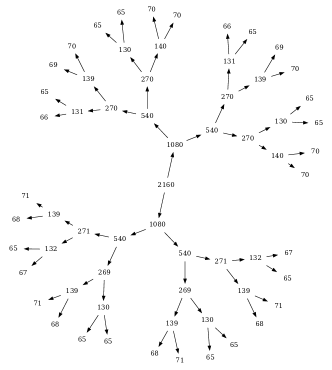
Figure 1: DoF cluster tree for a small hierarchical matrix corresponding to roll A consisting of 2160 monomers. The numbers in the tree indicate the number of DoF associated with each node of the tree. Each node in the tree represents a cluster of molecules (also DoF) in the problem structure.

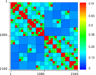
Figure 2: Compression ratio, defined as $k\frac{m+n}{mn}$ plotted for a relatively small hierarchical matrix corresponding to roll A consisting of 2160 monomers.

Hierarchical matrices were originally applied to reduce the computational complexity associated with the discretization of elliptic differential equations Borm et al. (2003); Hackbusch (1999). It has been shown that for matrices resulting from the discretization of elliptic partial differential equations the $\mathcal{H}\textnormal{-matrix }$method leads to the almost linear complexity of $\mathcal{O}(N\log(N))$ Borm et al. (2003); Hackbusch (1999); Hackbusch and Khoromskij (2000) which is clearly advantageous over the $\mathcal{O}(N^{2})$ complexity arising from the direct storage of the matrices. Although, the favorable properties of the $\mathcal{H}\textnormal{-matrix }$method will be lost if it is applied to non-elliptic operators, the method still provides very desirable performance in the so-called low frequency regime, i.e. when dimensions of the physical problem are smaller or comparable to the wavelengthBanjai and Hackbusch (2008). Owing to their submicron dimensions, many molecular aggregates give rise to problems that exactly fit in to the low-frequency category. The details of the $\mathcal{H}\textnormal{-matrix }$method can be found in Borm et al. (2003); Hackbusch (1999); Hackbusch and Khoromskij (2000); Borm et al. (2006) and will not be discussed here. Here it suffices to mention that in the $\mathcal{H}\textnormal{-matrix }$method, matrices are hierarchically reordered and segmented into blocks that are classified into near-field and far-field interaction blocks. The resulting near-field interaction blocks are stored as regular dense matrices while the far-field interaction blocks are stored via low rank representation. In other words, a far-field interaction block $\mathsf{M}_{m\times n}$ is decomposed into a truncated SVD-like decomposition $\mathsf{M\approx U\Sigma V}^{\dagger}$ in which singular values below a certain accuracy threshold are discarded. In practice, the low rank representation consists of a left factor $\mathsf{A}_{m\times k}$ and a right factor $\mathsf{B}_{n\times k}$ satisfying $\mathsf{M\approx AB}^{\dagger}$ where $k\ll\frac{mn}{m+n}$. The fact that $k\ll\frac{mn}{m+n}$ guarantees that storage and other operations such as matrix-vector multiplication operations can be handled with a significantly reduced cost compared to that of regular dense matrix representationBorm et al. (2003). An example of a hierarchical subdivision of DoF and the corresponding hierarchical matrix is depicted in Fig. 1 and Fig. 2 respectively. In Fig. 2 both the structure and the achieved compression ratio defined as $k\frac{m+n}{mn}$ can be observed. As can be seen, the near diagonal part of the matrix converts most of the self and near interactions and has the lowest levels of compression.

The time domain solution of the problem can be obtained by applying FFT to a large collection of frequency dependent solutions. Considering that a small number of Krylov iterations are needed for the problem solution at each frequency, most of the computational cost will be associated with the construction of the $\mathcal{H}\textnormal{-matrices }$. Hence, one may naturally think of interpolating the majority of these frequency dependent $\mathcal{H}\textnormal{-matrices }$from a limited set generated at a selected frequencies. Note that here the term ‘interpolation’ is used in its loose sense and shall imply the meaning of any curve fitting or parameterization technique. In the following section, an efficient parameterization method for $\mathcal{H}\textnormal{-matrices }$is proposed.

IV Parametric $\mathcal{H}\textnormal{-matrix }$Representation

Let us consider a block of the system matrix ${\mathsf{Z}}_{(m\times n)}$. We intend to build a frequency dependent characterization of the complete system matrix. The characteristic to our problem of interest, $\mathsf{Z}(f)$, is a smooth and infinitely differentiable function, except near the frequency points in the vicinity of the quantum mechanical resonances of individual monomers as discussed in section II. Due, to the presence of such singularities (poles) in the frequency representation of individual matrix entries, polynomial interpolation or polynomial least squares curve fitting methods are not applicable. Nonetheless, a rational function representation can effectively represent the individual matrix entries. Such a rational function representation can be obtained using the vector fitting method Gustavsen and Semlyen (1999); Chinea (2010). Thus, if the system matrix is represented in a dense form, the entries can be fitted to rational functions by means of the abovementioned method. Nevertheless, for large systems the computational complexity of the dense matrix representation is prohibitive.

Alternatively, in the $\mathcal{H}\textnormal{-matrix }$representation, two types of blocks are present: (1) dense blocks in the form of $\mathsf{M}$ used for near interactions (2) low rank (compressed) blocks $\mathsf{M}=\mathsf{A}\mathsf{B}^{\dagger}$. The dense blocks can be fitted directly into a rational function of frequency using the vector fitting method. On the other hand, for the low rank blocks, the frequency parameterization cannot be directly applied to the $\mathsf{A}$ and $\mathsf{B}^{\dagger}$ factors. In other words, direct interpolation/parameterization of $\mathsf{A}(f)$ and $\mathsf{B}(f)$ for the low rank blocks would result in undesirable results since the smoothness of $\mathsf{A}(f)$ and $\mathsf{B}(f)$ is not guaranteed, although the product $\mathsf{M}=\mathsf{A}\mathsf{B}^{\dagger}$ is known to be sufficiently smooth. This is because the matrices $\mathsf{A}(f)$ and $\mathsf{B}(f)$ are not unique, i.e. if $\mathsf{M}=\mathsf{A}\mathsf{B}^{\dagger}$, so will $\mathsf{M}=(\mathsf{A}\mathsf{C})(\mathsf{C}^{-1}\mathsf{B}^{\dagger})$ for any $\mathsf{C}\in\mathbb{C}^{k\times k},\det\mathsf{C}\neq 0$, $\mathsf{C}^{\dagger}=\mathsf{C}^{-1}$. Furthermore, redundancies may exist between the members of the sets $\{\mathsf{A}_{1},\mathsf{A}_{2},\cdots,\mathsf{A}_{n_{f}}\}$ and $\{\mathsf{B}_{1},\mathsf{B}_{2},\cdots,\mathsf{B}_{n_{f}}\}$ that respectively represent the range and the domain spaces of the frequency dependent matrix ${\mathsf{M}}$ at a selection of frequencies $\{f_{1},f_{2},\ldots,f_{n_{f}}\}$.

Suppose $n_{f}$ sampling frequencies are given as the key data points for the intended parameterization and thus the low rank representation of $\mathsf{M}$ using $\{\mathsf{A}_{1},\ldots,\mathsf{A}_{n_{f}}\}$ and $\{\mathsf{B}_{1},\ldots,\mathsf{B}_{n_{f}}\}$ is given. As one moves from $f_{p}$ to $f_{q}$, the range space of the operator $\mathsf{M}$ changes from $\mathsf{A}_{p}$ to $\mathsf{A}_{q}$. However, due to the finite dimension and the smooth frequency dependence of operator $\mathsf{M}$, it is expected that the range spaces of $\{\mathsf{A}_{1},\ldots,\mathsf{A}_{n_{f}}\}$ share common information. In order to extract the potentially existing redundancies in the set $\{\mathsf{A}_{1},\ldots,\mathsf{A}_{n_{f}}\}$, the SVD can be applied as

$$\{\mathsf{A}_{i,(m\times k_{i})}\}\rightarrow$$

$$[\mathsf{A}_{1},\ldots,\mathsf{A}_{n}]_{(m\times\sum k_{i})}=\mathsf{U}_{L,(m\times m)}\mathsf{\Sigma}_{L}\mathsf{V}^{\dagger}_{L,(\sum k_{i}\times\sum k_{i})},$$ (14)

where $\{\mathsf{A}_{i,(m\times k_{i})}\}$ is a set of range-space matrices and the subscript L denotes its association with left factor $\mathsf{A}$ in the original decomposition of $\mathsf{M}$. With a desired level of accuracy, the above SVD can be truncated and written as

$$[\mathsf{A}_{1},\ldots,\mathsf{A}_{n}]\approx\mathsf{\bar{U}}_{L,(m\times k_{L})}\mathsf{\bar{V}}_{L,(k_{L}\times\sum k_{i})}^{\dagger}.$$ (15)

Under the same truncation tolerance, each of the $\mathsf{A}_{i}$ matrices can be decomposed as $\mathsf{A}_{i,(m\times k_{i})}=\mathsf{\bar{U}}_{L,m\times k_{L}}\mathsf{V}_{L,i,(k_{L}\times k_{i})}^{\dagger}$, where $\mathsf{V}_{L,i}$ represents the portion of row vectors in $\mathsf{\bar{V}}_{L}$ that corresponds to the construction of $\mathsf{A}_{i}$. Applying a similar procedure to the right side factor, $\{\mathsf{B}\}_{i}$, we get

$$\left[\begin{array}[]{c}\mathsf{B}^{\dagger}_{1}\\ \vdots\\ \mathsf{B}^{\dagger}_{n}\\ \end{array}\right]_{(\sum k_{i}\times n)}\approx\mathsf{\bar{U}}_{R,(\sum k_{i}\times k_{R})}\mathsf{\bar{V}}_{R,(k_{R}\times n)}^{\dagger}.$$ (16)

Again, each $\mathsf{B}_{i}$ matrix is written as $\mathsf{B}_{i,(k_{i}\times n)}^{\dagger}\approx\mathsf{\bar{U}}_{R,i,(k_{i}\times k_{R})}\mathsf{\bar{V}}_{R,(k_{R}\times n)}^{\dagger}$, where $\mathsf{\bar{U}}_{R,i}$ represents the collection of row vectors in $\mathsf{\bar{U}}_{R}$ corresponding to the construction of $\mathsf{B}_{i}$. Now, one can state that

$$\mathsf{M}_{i}\approx\mathsf{\bar{U}}_{L}\mathsf{T}_{i}\mathsf{\bar{V}}_{R}^{\dagger},$$ (17)

where

$$\mathsf{T}_{i,(k_{L}\times k_{R})}\triangleq\mathsf{\bar{V}}_{L,i,(k_{L}\times k_{i})}^{\dagger}\mathsf{\bar{U}}_{R,i,(k_{i}\times k_{R})}$$ (18)

is only a frequency dependent part in the low rank representation of the block $\mathsf{M}_{i}$. The $\mathsf{T}_{i}$ matrix: (1) is unique for each frequency, and (2) it has smaller dimensions compared to the matrices $\mathsf{M}_{i}$, $\mathsf{A}_{i}$ and $\mathsf{B}_{i}$. Thus, lending itself to more efficient computational operations.

V Error Control

Errors in the parametric hierarchical matrix representation can be divided into two main categories: (a) truncation errors and (b) parameterization errors, where the former are associated with the low rank representations used in the $\mathcal{H}\textnormal{-matrix }$and the latter correspond to the parameterization (interpolation or curve fitting) procedure. There are no truncation errors for dense blocks. Thus, only parameterization errors should be minimized. For low rank blocks, however, some care must be taken to properly control both parameterization and truncation error while imposing minimal computational costs. For this purpose, let us consider the following parametric representation of a low rank block $\mathsf{M}(f)$

$$\mathsf{M}(f)=\mathsf{U}_{L}\mathsf{\Sigma}_{L}\mathsf{T}(f)\mathsf{\Sigma}_{R}\mathsf{V}^{\dagger}_{R},$$ (19)

where we assume that no SVD truncation has been applied to the left and right factors $\mathsf{U}_{L}\mathsf{\Sigma}_{L}$ and $\mathsf{\Sigma}_{R}\mathsf{V}^{\dagger}_{R}$.

In order to model the truncation error, assume that $\mathsf{\Delta\Sigma}_{L}$ and $\mathsf{\Delta\Sigma}_{R}$ represent the part of the singular value spectrum that is eventually removed due to the low rank representation. Also, let’s assume that a $\mathsf{\Delta T}$ error is introduced to the matrix $\mathsf{T}$ due to the parameterization. Then, the parameterized low rank representation is

$$\bar{\mathsf{M}}=\mathsf{U}_{L}(\mathsf{\Sigma}_{L}-\mathsf{\Delta\Sigma}_{L})(\mathsf{T}+\mathsf{\Delta T})(\mathsf{\Sigma}_{R}-\mathsf{\Delta\Sigma}_{R})\mathsf{V}^{\dagger}_{R}.$$ (20)

Assuming that all three sources of error, i.e. $\mathsf{\Delta\Sigma}_{L}$, $\mathsf{\Delta\Sigma}_{R}$ and $\mathsf{\Delta T}$ are small relative to their central values, and applying the Frobenius norm as an error measure we can write

$${|\!|e|\!|}_{F}\approx{|\!|\-\mathsf{\Delta\Sigma}_{L}\mathsf{T}\mathsf{\Sigma}_{R}-\mathsf{\Sigma}_{L}\mathsf{T}\mathsf{\Delta\Sigma}_{R}+\mathsf{\Sigma}_{L}\mathsf{\Delta T}\mathsf{\Sigma}_{R}|\!|}_{F}.$$ (21)

In ​​ 21 only terms linear in the error, i.e. lowest order perturbations, are included and the unitary matrices, $\mathsf{U}$ and $\mathsf{V}^{\dagger}$ are discarded due to the invariance of the Frobenius norm upon a unitary transformation. The upper bound for the error, ​​ 21, can be derived using the triangle inequality

$${|\!|-\mathsf{\Delta\Sigma}_{L}\mathsf{T}\mathsf{\Sigma}_{R}-\mathsf{\Sigma}_{L}\mathsf{T}\mathsf{\Delta\Sigma}_{R}+\mathsf{\Sigma}_{L}\mathsf{\Delta T}\mathsf{\Sigma}_{R}|\!|}_{F}\leq$$

$${|\!|\mathsf{\Delta\Sigma}_{L}\mathsf{T}\mathsf{\Sigma}_{R}|\!|}_{F}+{|\!|\mathsf{\Sigma}_{L}\mathsf{T}\mathsf{\Delta\Sigma}_{R}|\!|}_{F}+{|\!|\mathsf{\Sigma}_{L}\mathsf{\Delta T}\mathsf{\Sigma}_{R}|\!|}_{F}.$$ (22)

The three terms in the above expression indicate that there are three sources of error, two related to the truncation of the left and the right factors and one coming from the error caused by parametrization of matrix entries. The truncation error contributions can be controlled through proper truncation of singular values in the left and right factors, pretty much as it is done for the low rank blocks in non-parametric hierarchical matrices. This bound serves as a convenient measure of the accuracy of the parametric $\mathcal{H}\textnormal{-matrix}$ blocks and can be used for assessment of the success of the parametrization.

Moreover, the $\mathsf{\Sigma}_{L}\mathsf{\Delta T}\mathsf{\Sigma}_{R}$ directly reflects how the error due to the parameterization procedure is manipulated by the left and right factors, i.e. $\mathsf{\Sigma}_{L}$ and $\mathsf{\Sigma}_{R}$. The immediate consequence, however, is that not all entries in $\mathsf{T}$ need to have the same level parameterization error as these entries are scaled by the singular values in $\mathsf{\Sigma}_{L}$ and $\mathsf{\Sigma}_{R}$. Therefore, in order to control the parameterization error in $\mathsf{T}$, one needs not to directly control the error in the individual entries $\mathsf{T}_{ij}$, but rather that of $\mathsf{\Sigma}_{L,ii}\mathsf{T}_{ij}\mathsf{\Sigma}_{R,jj}$. In other words, the error introduced due to the parameterization of the $\mathsf{T}_{ij}$ entries with higher values of $i$ and $j$ is less important as it will be multiplied by smaller singular values. In practice, this balances out with the more significant error level that is observed in the parameterization error induced $\mathsf{T}_{ij}$ entries with higher values of $i$ and $j$. In this light, the individual entries of the $\mathsf{T}$ matrix can be observed as the modal functions from which the matrix block $\mathsf{M}$ is constructed as a function of frequency. Intuitively, one observes that the modal functions with higher indices have more complicated behavior and thus are more difficult to parameterize.

VI Chlorosome Roll Model

It is understood that the chlorosome is composed of multiple rolls and curved lamella structures as schematically illustrated in Fig. 3(a). While there are several models for BChl packing in the aggregates Holzwarth and Schaffner (1994); Pcencik et al. (2004); Ganapathy et al. (2009), we use the one suggested recently by Ganapathy et. al. Ganapathy et al. (2009). The lowest electronic excitation in single BChls, $Q_{y}$ band, is about 1.8 eV or 435 THz with the orientation of the transition dipole shown in Fig. 3(b). The $Q_{y}$ band is separated sufficiently from the next transition, $Q_{x}$ band. Thus, in our modeling only the lowest electronic excitation is considered. According to the model Ganapathy et al. (2009) BChl pigment molecules are arranged in concentric rings and then stacks of these rings form a roll. The molecular transition dipoles are almost orthogonal to the radius and form 35 degrees angle with the plane of the ring. Fig. 3 (c) schematically depicts the molecular structure of one of the rolls consisting of the bacteriochlorophyll molecules depicted in Fig. 3(b).

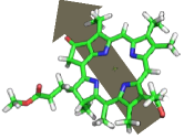
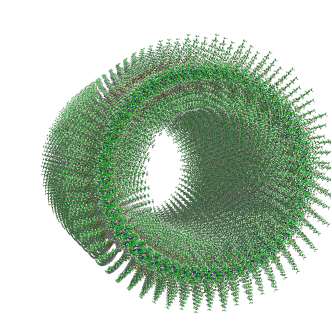
Figure 3: (a) A schematic structure of the chlorosome antenna in green sulfur bacteria. Tubular and curved lamella aggregates of pigment bacteriochlorophyll molecules form an ovoid-shaped body with characteristic size of tens to hundreds of nanometers. (b) A bacteriochlorophyll molecule with the orientation of the lowest transition dipole shown. (c) Packing of BChl transition dipoles in a roll aggregate forms a collection of infinitesimally small electrical dipoles.

To model the chlorosome response four concentric rolls A, B, C and D with $N_{A-D}=60,80,100,120$ number of molecules per ring (see Fig. 9 for details), and $n=36$ rings were constructed and their structure was compared to the structures provided to us by the authors of reference Ganapathy et al. (2009). The molecular structure depicted in Fig. 3 (c) corresponds to the innermost roll A. For transient response calculations, we selected six points (and monomers) $a-f$ coinciding some of the monomers in the four-roll structure. Points $a$,$c$ ($d$,$f$) are located on the edges of the inner (outer) rolls, and points $b$ and $e$ belong to the central rings of the same rolls, as shown in Fig. 9. Clearly, the line shifts associated with the retardation cannot be observed at ambient conditions, where the resonance lines are broadened by about 50 meV due to the structural disorder and thermal effects. However, the role of disorder in the intensity redistribution cannot be easily analysed and should be studied in more detail.

We illustrate the developed computational method by modeling the optical responses of BChl roll aggregates, contained in the chlorosome antenna complex of green photosynthetic bacteria Oostergetel et al. (2010). All results presented in this article were obtained using a C++ code compiled with the GNU C++ version $4.6.3$ compiler on a Linux based dual 6-core Intel Xeon 5649 workstation although the muti-core features of the machine were not used in our current implementation. All reported timings are based on single-thread runs without parallelization.

VI.1 Spectral analysis

As a first step we compared the resonance spectra of roll D in Fig. 9 simulated using the hybrid quantum-classical formulation with that of the quantum Hamiltonian model Fujita et al. (2012) calculated as described in referenceSomsen et al. (1996). The hybrid model used in this article, takes the quantum mechanical effects into account via the polarizability factor of individual monomers, while the interaction between molecules is considered within a self-consistent linear response theory. Figure 4 shows the spectra computed with both models, where the resonance frequency of isolated monomers $1.8$ eV was used as a baseline and the linewidth was assumed to be 0.1 meV in order to resolve different resonances. The resonances of the chlorosome aggregates are red-shifted from the monomer frequency in both quantum and hybrid model in agreement with the experimental data Oostergetel et al. (2010). Apart from a frequency shift attributed to the difference between the quantum and the classical model (and also due to the inclusion of retardation effects since the quantum model only accounts for the electrostatic interactions) the structures of the computed spectra are very similar. Please note that the difference in the spectra obtained by means of these models cannot be seen as a perfect red shift since larger shifts are observed at lower frequencies.

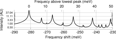
(a) Semiclassical model

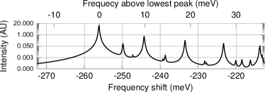
(b) Quantum model

Figure 4: Frequency spectra of roll D in response to $\hat{z}$-polarized optical field computed using a quantum mechanical and a hybrid electrodynamic method. The numbers on the bottom horizontal axis indicate the relative red shift in meV with respect to the resonant frequency of the individual molecules located at $1.8\textnormal{eV}$ which is equivalent to $435\textnormal{THz}$. In the semicalssical results, the vertical axis shows the sum of the squared polarization amplitudes of individual molecules. To enhance the details the vertical axis is in log scale.

Both electrodynamic and electrostatic formulations have been proposed previously to study the interaction of light with molecular aggregates DeVoe (1965); Keller and Bustamante (1986); Zimanyi and Silbey (2010). Intuitively, when the physical dimension of the structure is much smaller than the wavelength of light, electrodynamic retardation effects are expected to be insignificant. However, as the dimensions of the structure increase and become comparable with the wavelength, those effects can become more pronounced. For this purpose, we constructed an long roll that has the same radius as roll D but length $290\textnormal{ nm}$, which is comparable to the physical length of a chlorosome Oostergetel et al. (2010). The resulting structure for this ‘extended roll D’ consists of $N=43200$ molecules. The obtained spectra, Fig. 5 and Fig. 6, show that the retardation effects can result in a sufficient redistribution of peak intensities within the aggregate especially for the fields polarized along the roll’s symmetry axis.

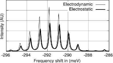
Figure 5: Frequency spectrum of the extended roll D in response to $\hat{x}$-polarized initial electric field using both electrostatic and electrodynamic formulation. The numbers on the bottom horizontal axis indicate the relative red shift in meV with respect to the resonant frequency of the individual molecules located at $1.8\textnormal{eV}$. The vertical axis shows the sum of the squared polarization amplitudes of individual molecules. To enhance the details the vertical axis is in log scale.

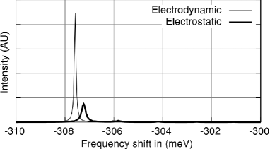
Figure 6: Frequency spectrum of the extended roll D in response to $\hat{z}$-polarized initial electric field using both electrostatic and electrodynamic formulation. The numbers on the bottom horizontal axis indicate the relative red shift in meV with respect to the resonant frequency of the individual molecules located at $1.8\textnormal{eV}$. The vertical axis shows the sum of the squared polarization amplitudes of individual molecules.

To examine the reliability of the parametric $\mathcal{H}\textnormal{-matrix }$method two example problems were solved using both the parametric $\mathcal{H}\textnormal{-matrix }$and the nonparametric $\mathcal{H}\textnormal{-matrix }$method. As a first example the bacteriochlorophyll roll of Fig. 9 was excited with a steady state plane wave and polarization intensities were calculated as a function of the excitation frequency. The excitation decay rate was assumed to be the same for all monomer with equal $\gamma=50$ meV. Fig. 7 shows a quantitative agreement between the response obtained by means of the parametric $\mathcal{H}\textnormal{-matrix }$method at 300 frequencies (in the 200 THz to 800 THz band) and twenty five sample points obtained using the $\mathcal{H}\textnormal{-matrix }$method. As a second example a similar comparison was done for the $290$ nm long roll, see Fig. 8, which again showed a perfect agreement between the results.

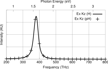
Figure 7: Response to plane wave excitation traveling along $\hat{z}$ and the electrical field polarized along $\hat{x}$. In the legend, ‘H’ and ‘pH’ indicate $\mathcal{H}\textnormal{-matrix }$and parametric $\mathcal{H}\textnormal{-matrix }$method respectively. The vertical axis shows the sum of the squared polarization amplitudes of individual molecules.

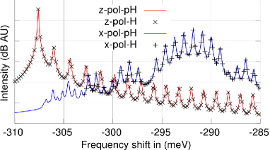
Figure 8: Comparison of the spectral response of extended roll D structure using both $\mathcal{H}\textnormal{-matrix }$and parametric $\mathcal{H}\textnormal{-matrix }$method. The response is due to initial field excitation along $\hat{z}$ direction. The vertical axis shows the sum of the squared polarization amplitudes of individual molecules. To enhance the details the vertical axis is in log scale.

VI.2 Transient Response of Roll Aggregates

Here, the chlorosome roll of Fig. 9 is excited with initial $\hat{z}$ polarized electric field incident on monomers located at the central ring of roll A, i.e. the innermost roll as illustrated in Fig. 9, and the time evolution of the polarization induced in various monomers at the points $a-f$ in the four-layer roll, see Fig. 9, is observed. The time domain is constructed from a large number of frequency domain solution via FFT. Thus it is natural to use the parametric $\mathcal{H}\textnormal{-matrix }$method to rapidly produce the required frequency response. The results presented in this section were obtained via $350$ frequency domain solutions covering the frequency band from 0 THz to 800 THz. The parametric $\mathcal{H}\textnormal{-matrix }$is produced from $13$ $\mathcal{H}\textnormal{-matrices }$evenly covering the 100 THz to 700 THz band. Generation of each $\mathcal{H}\textnormal{-matrix }$takes about $172$ seconds ($2236$ seconds total) and the construction of the parametric $\mathcal{H}\textnormal{-matrix }$takes another $2000$ seconds. However, when the parametric $\mathcal{H}\textnormal{-matrix }$is ready, the construction of each $\mathcal{H}\textnormal{-matrix }$at a given frequency only requires $7$ seconds. At most frequencies, very few ($4$ to $50$) Krylov iterations are needed for the matrix solution process and thus the computational time is mainly determined by the time spent on the construction of the system $\mathcal{H}\textnormal{-matrix }$. Under this configuration, the parametric $\mathcal{H}\textnormal{-matrix }$method leads to an overall speedup factor of $8$ compared to the direct use of the $\mathcal{H}\textnormal{-matrix }$method. It is worth mentioning that higher speedup factors will be achieved when a larger number of frequency domain solutions are required or when larger structures need to be solved.

Considering the symmetric geometry of the roll and the initial excitation similar time signatures are expected to occur at both (top and bottom) ends of the roll. However, comparing ‘d’ and ‘e’ in Fig. 10 it appears that the polarization dynamics at the two ends of the chlorosome roll is slightly different. This can be linked to the chiral nature of the roll although a more systematic examination of the problem is needed before definitive conclusions can be made. Also as can be seen in Fig. 10, the responses on the outmost sub-roll, i.e. sub-roll D, seem to have longer lifetimes which is likely to be consequence of larger radius of sub-roll D compared to sub-roll A.

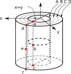
Figure 9: Location of observation monomers in the four-layer chlorosome roll. The letters a, b, c, d, e and f indicate the six monomers used for the observation of the time evolution of their polarization amplitude as depicted in Fig. 10. The capital letters A, B, C and D correspond to the four layers discussed in section VI.

(a) @ a

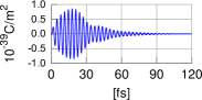
(b) @ d

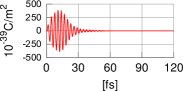
(c) @ b

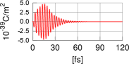
(d) @ e

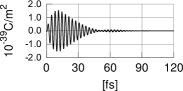
(e) @ c

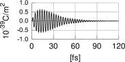
(f) @ f

Figure 10: Transient response (polarization amplitude) of various monomers in the four-layer roll in response to initial $\hat{z}$ oriented electrical field of amplitude 1 V/m, imposed on monomers 1049 to 1108 located on a circular ring at the center of the innermost roll. The alphabetical labels in the legend correspond to the probe monomers depicted in Fig. 9.

The estimated number of molecules in the whole chlorosome is of the order of $200,000-250,000$ Oostergetel et al. (2010), which is about 20 times larger that our four-layered roll model. In order to examine the performance of the presented parametric $\mathcal{H}\textnormal{-matrix }$technique for the structures comparable with the size of the chlorosome, we obtain the transient response of a 2 by 4 array of rolls with a lattice spacing of $25.5\textnormal{nm}$ along both $\hat{x}$ and $\hat{y}$ directions. The resulting structure consists of $103680$ monomers and thus each frequency solution involves construction and $\mathcal{H}-\textnormal{compression}$ of a $103680\times 103680$ matrix. Similar to section VI.2, a central ring of monomers located in roll 1 of the array is exposed to initial electrical field along $\hat{z}$ direction and then the response of the system (polarization) at various monomers is presented in Fig. 12 and Fig. 13.

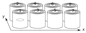
(a) side view

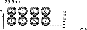
(b) top view

Figure 11: The 3D configuration of the $4\times 2$ roll array. The dotted line shows the location of the monomers exposed to initial electrical field.

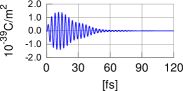
(a) @ a

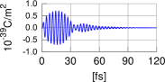
(b) @ d

(c) @ b

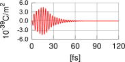
(d) @ e

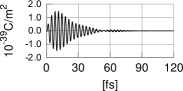
(e) @ c

(f) @ f

Figure 12: Transient response (polarization amplitude) of various monomers in chlorosome roll number $1$ in the array configuration illustrated in Fig. 11. The labels in the legend refer to observation monomers depicted in Fig. 9. The response is due to initial $\hat{z}$ oriented electrical field of amplitude 1 V/m, imposed on monomers 1049 to 1108 located in chlorosome roll number $1$.

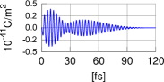
(a) @ a’

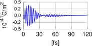
(b) @ d’

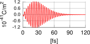
(c) @ b’

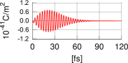
(d) @ e’

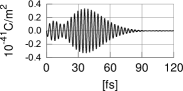
(e) @ c’

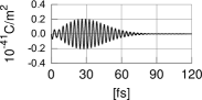
(f) @ f’

Figure 13: Transient response (polarization amplitude) of various monomers in chlorosome roll number $8$ in the array configuration illustrated in Fig. 11. The labels in the legend refer to the observation monomers depicted in Fig. 9 shifted into roll number $8$. The response is due to initial $\hat{z}$ oriented electrical field of amplitude 1 V/m, imposed on monomers 1049 to 1108 located in chlorosome roll number $1$.

VI.2.1 Computational Statistics

The statistics presented here correspond to the $2$ by $4$ array problem of section VI.2. A dense matrix representation in this case will require $103680\times 103680\times 16$ bytes (approximately 160 GB) of memory and thus immediately ruled out. In a general scenario, the computational times can divided into two parts, (1) construction of the system matrix and (2) the iterative solution of the problem. The iterative solution time is equal to the time required for one system matrix-vector multiply operation times the number of iterations needed for the desired accuracy. Thus, the two methods have equal performance in this part. An $\mathcal{H}\textnormal{-matrix }$representation of the system matrix using an accuracy threshold of $\epsilon=10^{-4}$ leads to a compressed representation of the system that requires abtout $8GB$ of memory. However, the construction of the compressed $\mathcal{H}\textnormal{-matrix }$takes $65$ to $70$ minutes per frequency. Hence, the construction of the system $\mathcal{H}\textnormal{-matrix }$at $350$ frequency points requires $350\times 65\times 60=1365000$ seconds. On the other hand, using the parameterized $\mathcal{H}\textnormal{-matrix }$method, $13$ $\mathcal{H}\textnormal{-matrices }$are constructed at 13 equally spaced frequencies ranging from 100 THz to 700 THz and then the parametric $\mathcal{H}\textnormal{-matrix }$is constructed from the samples. This process takes $13\times 65\times 60$ seconds for the initial $\mathcal{H}\textnormal{-matrices }$plus another $10$ hours for the construction of the parametric $\mathcal{H}\textnormal{-matrix }$. Thus the parametric $\mathcal{H}\textnormal{-matrix }$requires a total of $86700$ seconds. On top of that, at each frequency point, the $\mathcal{H}\textnormal{-matrix }$can be constructed from the parametric $\mathcal{H}\textnormal{-matrix }$in $80$ seconds leading to a speed up factor of $12$. Fig. 14 compares the growth of the computational times associated with the construction of the system matrix using both $\mathcal{H}\textnormal{-matrix }$and parametric $\mathcal{H}\textnormal{-matrix }$method. The curves depicted in Fig. 14 are the representation of two linear equations with a considerable difference between their slopes and constant terms. From the figure it can be seen that the parametric $\mathcal{H}\textnormal{-matrix }$method outperforms the $\mathcal{H}\textnormal{-matrix }$method when the problem needs to be solved at more than $20$ frequencies.

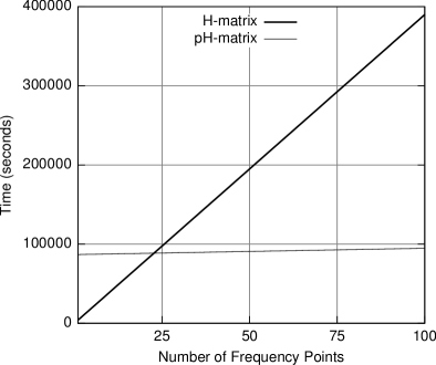
Figure 14: Comparison of the system matrix preparation times between the parametric and non-parametric $\mathcal{H}\textnormal{-matrix }$methods.

VII Conclusion

An $\mathcal{H}\textnormal{-matrix }$acceleration method is adopted for the classical formulation arising in the simulation of molecular aggregates. The $\mathcal{H}\textnormal{-matrix }$approach reduces the otherwise $\mathcal{O}(N^{2})$ complexity that arises from direct implementation of the resulting matrix problem. Moreover, a novel parametric $\mathcal{H}\textnormal{-matrix }$approach is introduced and provides an efficient means for the solution of large excitonic problems such as those encountered in the study of the photosynthesis process. A tubular aggregate of pigment molecules as used as an example to demonstrate that the developed method can give an order of magnitude acceleration in the calculations of transient responses as compared to the $\mathcal{H}\textnormal{-matrix }$approach. Further work on a detailed characterization of the physics of this model is in progress in our groups. Numerical experiments conducted in this work verify the validity of robustness of the method. Another important advantage of the parametric $\mathcal{H}\textnormal{-matrix }$method lies in the fact that it can easily be used for other kernels and thus other formulations including the quantum Hamiltonian method can also be accelerated using this technique. The scope of the applicability of the parametric $\mathcal{H}\textnormal{-matrix }$method goes beyond the current application as it can be applied to many other $\mathcal{H}\textnormal{-matrix }$compatible problems including those arising from the discretization of integral operators in other fields such as acoustics, electromagnetics, fluid mechanics and fracture mechanics. Future works will focus on enhancing the method via computer parallelization. In this work, the parameterization was used for efficient frequency sweeping, however, the approach can potentially be applied to other types of parameter sweeping.

VIII Acknowledgements

D. A.-O.-B., M. R.,E. C. and H. M. acknowledge US Air Force Office of Scientific Research (AFOSR) grant No. FA9550-10-1-0438 and in-part U.S. Office of Naval Research (ONR) MURI award grant N00014-10-1-0942. S. K. S., S. V., and A. A.-G. acknowledge Defense Threat Reduction Agency grant HDTRA1-10-1-0046 and Defense Advanced Research Projects Agency grant N66001-10-1-4063. Further, A. A.-G. is grateful for the support from the Corning Foundation.

References

- Saikin et al. (2013) S. K. Saikin, A. Eisfeld, S. Valleau, and A. Aspuru-Guzik, Nanophotonics 2, 21 (2013).
- Blankenship (2002) R. E. Blankenship, Molecular mechanisms of photosynthesis (Blackwell Science Ltd, 2002).
- Lidzey et al. (1999) D. G. Lidzey, D. D. C. Bradley, T. Virgili, A. Armitage, M. S. Skolnick, and S. Walker, Phys. Rev. Lett. 82, 3316 (1999).
- Fofang et al. (2008) N. T. Fofang, T.-H. Park, O. Neumann, N. A. Mirin, P. Nordlander, and N. J. Halas, Nano Lett. 8, 3481 (2008).
- Würthner et al. (2011) F. Würthner, T. E. Kaise, and C. R. Saha-Möller, Angew. Chem. Int. Ed. 50, 3376 (2011).
- Bradley et al. (2005) M. Bradley, J. Tischler, and V. Bulovic, Adv. Mater. 17, 1881 (2005).
- Kirstein and Daehne (2006) S. Kirstein and S. Daehne, Int. J. Photoenergy p. 20363 (2006).
- Roden et al. (2010) J. Roden, W. T. Strunz, and A. Eisfeld, Int. J. Mod. Phys. B 24, 5060 (2010).
- Shim et al. (2012) S. Shim, P. Rebentrost, S. Valleau, and A. Aspuru-Guzik, Biophys. J. 102, 649 (2012).
- DM et al. (2012) E. DM, C. CW, B. EA, V. SM, van der Kwaak CGF, S. RJ, K. J. Bawendi MG and, R. JP, and V. B. DA, Nature Chemistry 4, 655 (2012).
- DeVoe (1965) H. DeVoe, J. Chem. Phys. 43, 3199 (1965).
- Keller and Bustamante (1986) D. Keller and C. Bustamante, J. Chem. Phys. 84, 2961 (1986).
- Zimanyi and Silbey (2010) E. N. Zimanyi and R. J. Silbey, Journal of Chemical Physiscs 133, 144107 (2010).
- Roden et al. (2009) J. Roden, G. Schulz, A. Eisfeld, and J. Briggs, Journal of Chemical Physiscs 131, 044909 (2009).
- Coifman et al. (1993) R. Coifman, V. Rokhlin, and S. Wandzura, IEEE Trans. Ant. Prop. 35, 7 (1993).
- Seo and Lee (2005) S. M. Seo and J.-F. Lee, IEEE Trans. Magn. 41, 1476 (2005).
- Borm et al. (2003) S. Borm, L. Grasedyckb, and W. Hackbusch, Engineering Analysis with Boundary Elements 27, 406 (2003).
- Hackbusch (1999) W. Hackbusch, Computing 62, 89 (1999).
- Fujita et al. (2012) T. Fujita, J. C. Brookes, S. K. Saikin, and A. Aspuru-Guzik, J. Phys. Chem. Lett. 3, 2357 (2012).
- Yurkin and Hoekstra (2007) M. A. Yurkin and A. G. Hoekstra, Journal of Quantitative Spectroscopy and Radiative Transfer 106, 558 (2007).
- Saad (2003) Y. Saad, Iterative Methods for Sparse Linear Systems, Second Edition (SIAM, 2003).
- Banjai and Hackbusch (2008) L. Banjai and W. Hackbusch, IMA Journal of Numer. Anal. 28, 46 (2008).
- Yaghjian (1980) A. D. Yaghjian, Proceedings of the IEEE 68, 248 (1980).
- Jackson (1999) J. Jackson, Classical Electrodynamics, vol. 1 (John Wiley & Sons, Inc., 1999).
- Hackbusch and Khoromskij (2000) W. Hackbusch and B. Khoromskij, Computing 64, 21 (2000).
- Borm et al. (2006) S. Borm, L. Grasedyckb, and W. Hackbusch, Tech. Rep. 21, Max-planck Institue fur Mathematik in den Naturwissenschaften Leipzig (2006).
- Gustavsen and Semlyen (1999) B. Gustavsen and A. Semlyen, IEEE Trans. Power Del. 14, 1052 (1999).
- Chinea (2010) A. Chinea, in Electrical Performance of Electronic Packaging and Systems (EPEPS), 2010 IEEE International Symposium on (2010).
- Holzwarth and Schaffner (1994) A. R. Holzwarth and K. Schaffner, Photosynth. Res. 41, 225 (1994).
- Pcencik et al. (2004) J. Pcencik, T. P. Ikonen, P. Laurinmäki, M. C. Merckel, S. J. Butcher, R. E. Serimaa, and R. Tuma, Biophys. J. 87, 1165 (2004).
- Ganapathy et al. (2009) S. Ganapathy, G. Oostergetel, P. Wawrzyniak, M. Reus, A. Gomez Maqueo Chew, F. Buda, E. Boekema, D. Bryant, A. Holzwarth, and H. de Groot, Proc. Natl. Acad. Sci. 106, 8525 (2009).
- Oostergetel et al. (2010) G. T. Oostergetel, H. v. Amerongen, and E. J. Boekema, Photosynth Res 104, 245 (2010).
- Somsen et al. (1996) O. J. G. Somsen, R. van Grondelle, and H. van Amerongen, Biophys. J. 71, 1934 (1996).